23.2 Fake (synthetic) depth of field🔗⧉

A large-sensor camera with a fast lens isolates its subject by physics: the background falls outside a shallow depth of field and dissolves into the soft, structured blur the last chapter dissected. A phone usually produces less optical background blur for a comparable portrait, though close focus or a telephoto module can still give visible defocus. Its sensor is fingernail-sized and its lens is correspondingly short, and (by the sensor-size scaling FUNDAMENTALS derived and Chapter 23.1, Bokeh, focus stacking, and depth-of-field control restated) that combination gives it an enormous depth of field in which almost everything is sharp at once. For snapshots this is a gift; for portraits it reads as flat, busy, un-cinematic. So the phone does in software what the glass cannot do in hardware: it estimates the scene's depth (or at least which pixels are the subject), then synthesizes the background blur, growing the blur with defocus and shaping it like a real aperture. This is fake, or synthetic, depth of field, the effect usually marketed as portrait mode. It is the computational counterpart to the optical depth of field of the previous chapter, and the whole of it is a pipeline whose stages we take in turn: why phones must fake it, where the depth comes from, how depth becomes a blur radius, why a Gaussian betrays the fake, how occlusion is handled, and where it all breaks.

23.2.1 Why phones must fake it🔗⧉

The root cause is the capture geometry. At matched viewpoint, framing, f-number, and final viewing size, a smaller sensor uses a shorter focal length and gives greater depth of field. These are linked quantities, not two independent causes. A wider entrance pupil can reduce depth of field, but the aperture needed to match a large-format fast portrait lens may be impractical in a phone. Phones can produce optical defocus, especially close up; portrait mode extends its strength and flexibility beyond what a particular module captures.

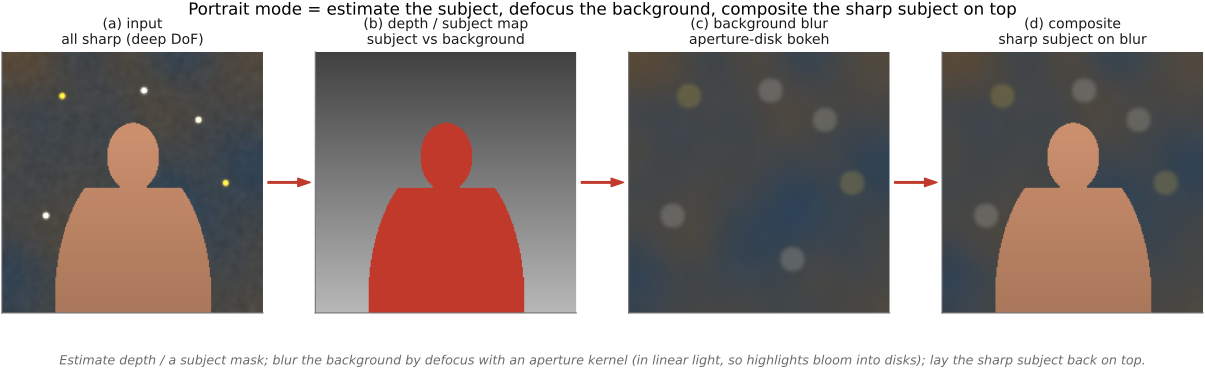
What photographers want from a portrait, though, is exactly the opposite: the subject isolated, lifted off a soft background that does not compete for attention. Since the optics refuse to deliver it, the phone computes it. "Portrait mode" estimates where each pixel sits in depth (or, more cheaply, simply which pixels belong to the subject and which to the background) and then blurs everything that is not the subject by an amount that grows with its distance from a chosen virtual focal plane, painting in a believable aperture-shaped blur as it goes (Figure 23.2.1⛶ fullscreen). The output is a picture meant to resemble one from a large sensor and a fast lens, assembled from one that did neither. This is the computational sibling of the optical Chapter 23.1, Bokeh, focus stacking, and depth-of-field control chapter. It aims for the same visual result by different means.

The idea predates portrait mode by a decade. An early take was defocus magnification Bae & Durand 2007 (Defocus Magnification): from a single small-sensor photo, estimate the slight defocus blur already present at each edge, use it as a cheap proxy for depth, and then magnify it to fake a shallower depth of field. The technique provides an instructive alternative to the dual-pixel, stereo, and learned depth cues used in later systems but it is the conceptual ancestor of everything in this chapter: measure what little defocus cue a small camera does have, and amplify it into the look of a big one.

23.2.2 Where the depth (or subject) comes from🔗⧉

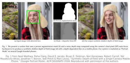
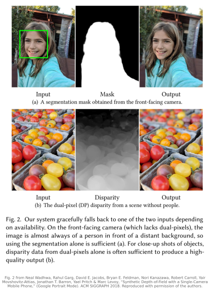
A synthetic blur is only as faithful as the depth that drives it, and there are four places a phone can get that depth, in rough order of hardware cost. The first is dual-pixel disparity. As Chapter 22.9, Autofocus explained, a dual-pixel sensor splits every photosite into two half-photodiodes under one microlens, so the left and right halves see the left and right halves of the lens's pupil, a stereo pair with an effective baseline determined by the separated pupil regions inside a single lens. Correlating the left-half image against the right-half image gives a dense, if shallow, per-pixel disparity, and the signed disparity constrains defocus relative to the current focus setting. Converting it to depth requires calibration and becomes uncertain when disparity is small. This is precisely the signal Wadhwa et al. exploited in their 2018 Synthetic Depth-of-Field with a Single-Camera Mobile Phone Wadhwa et al. 2018, the basis of Google's single-camera Portrait mode, which extracts a usable depth map from one lens by reading the dual-pixel split.

The second source is multi-camera stereo: a phone with two rear lenses has a real (if small) baseline between them, and the classic two-view matching of Chapter 12.3, Sparse matching yields a depth map, subject to the usual headaches of textureless regions and half-occluded pixels that any stereo system fights. Because the baseline is short and the match must run on a power budget, fast approximate solvers matter; Barron et al.'s 2015 Fast Bilateral-Space Stereo Barron et al. 2015 is the canonical move here, solving the stereo (and the subsequent edge-aware depth smoothing) in a bilateral space so that the depth snaps to image edges cheaply enough to run on a phone. The third source needs no special hardware at all: monocular depth networks that predict depth from a single image, the subject of Chapter 36.3, Monocular depth estimation (one image → depth). They are metrically loose (they recover relative depth far better than absolute distance) but for a blur whose only job is to look plausible, relative depth ordering is most of what matters.

The fourth source is a practical shortcut, often combined with the other cues: segmentation and matting. Often a full depth map is overkill, because the photographer only wants "the person sharp, everything else soft." A clean subject mask (a person-segmentation network, refined into a soft alpha matte as in Compositing, segmentation and matting) suffices to blur everything that is not the subject, with no per-pixel depth at all. The cost is that the background is then blurred uniformly rather than progressively by distance, so a far wall and a near shoulder behind the subject get the same blur; the gain is robustness and speed. In practice a production portrait mode blends these sources (dual-pixel or stereo depth where it is reliable, a learned matte to nail the subject's silhouette, a monocular net to fill the gaps) because each works best in cases where the others are less reliable.

23.2.3 From depth to blur: the thin-lens circle🔗⧉

Given a depth (or subject) map, an ideal thin-lens model supplies a useful mapping to blur size. Choose a virtual focal plane at depth $z_f$, usually the subject's distance, and give each pixel a blur kernel whose radius grows with how far that pixel's depth $z$ departs from the focal plane. This is the same circle-of-confusion law that governs a real lens, imported wholesale from Chapter 23.1, Bokeh, focus stacking, and depth-of-field control and FUNDAMENTALS:

The proportionality constant rolls up the chosen virtual aperture and focal length: it is the knob the "blur strength" slider turns. The structure of the formula is what matters: a pixel at the focal plane ($z = z_f$) gets zero blur and stays razor sharp; a pixel far behind the subject gets a large kernel; and because of the reciprocals, the blur grows asymmetrically: an equally distant displacement in front of focus produces more blur than one behind, since inverse depth changes faster nearby. Background blur approaches a finite limit as $z$ tends to infinity. A phone can evaluate this per pixel trivially fast.

That is the whole of the easy part, and the equation itself is straightforward; the difficulty lies in the surrounding stages. The thin-lens law supplies a geometric blur size under its assumptions; it tells you nothing about the shape of the kernel (the next section), nothing about what happens at the silhouette where a sharp subject meets a blurred background (the section after), and it presupposes a depth map whose accuracy at edges is precisely where the depth sources above are least trustworthy. The circle-of-confusion mapping is the least contentious stage of the pipeline, but an incorrect depth scale or arbitrary radius clamp can make even this mapping visibly wrong.

23.2.4 Realistic bokeh: why a Gaussian looks fake🔗⧉

A Gaussian often fails to reproduce the appearance of an aperture-shaped defocus highlight. Its smooth bell has neither the approximately uniform interior of an ideal circular pupil image nor a polygonal iris boundary. Real bokeh can also be soft-edged because of apodization or aberration, so a hard disk is not universally correct. Both a normalized Gaussian and a normalized disk spread a point's energy and reduce its peak. The conspicuously bright disks in photographs often come from sources whose radiance greatly exceeded the saturation level of the sharp input image. Clipping has discarded that excess; blurring the clipped image cannot recover it (Figure 23.2.4⛶ fullscreen).

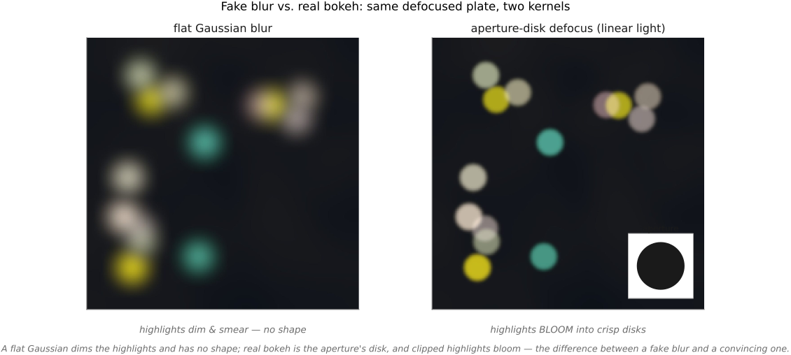
Scatter and gather are two ways to evaluate a blur operator. A scatter renderer visits each source pixel and distributes its contribution through a kernel determined by that source's depth. A gather renderer visits each output pixel and sums the source contributions that reach it. If both implement the same weights and visibility, they produce the same image; energy conservation is not exclusive to scatter. For an unoccluded source splat, normalize its kernel to total weight one. Neither that normalization nor switching loop order restores radiance lost to clipping.

The implementation tradeoff is real. Scatter creates overlapping writes and often needs atomics or tiled accumulation on a GPU; gather has more regular output writes but must search the correct source footprints rather than apply only the destination pixel's radius. Depth boundaries require visibility in either implementation. Process radiance in linear light, retain HDR values when available, and treat highlight boosting from an LDR input as an artistic estimate. Learned bokeh renderers, including work in the AIM Bokeh Effect Rendering challenges, can learn appearance and edge handling jointly, but their output still depends on training data and the information in the capture.

23.2.5 Occlusion-aware compositing and matting🔗⧉

Here the main caveat from Chapter 23.1, Bokeh, focus stacking, and depth-of-field control matters directly: defocus is not a 2-D convolution. A real lens does not blur the flat image; it blurs the scene, in depth, and at every depth discontinuity the geometry is subtle. A sharp foreground subject must occlude the background behind it: the background's blur grows right up to the subject's silhouette and stops, while the crisp subject sits cleanly on top. Run a naive whole-image blur instead, and the subject's own sharp edge gets dragged outward into the blur, painting a tell-tale bright or dark halo around the person, the single most recognizable artifact of a bad portrait fake (Figure 23.2.5⛶ fullscreen).

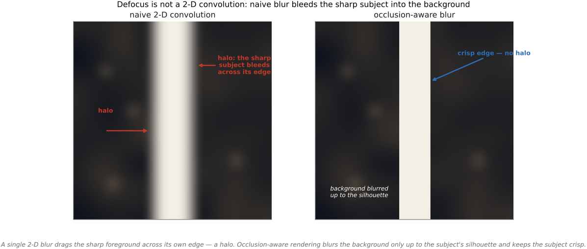
The fix is to render in depth order, as layers, rather than convolving the image as a single sheet. Estimate foreground color, alpha coverage, and a completed background; a matte alone does not supply those hidden colors. Blur the completed background and composite the sharp premultiplied foreground over it. For a defocused foreground, blur its premultiplied color and alpha consistently before compositing, so the subject's edge is never smeared into the blur. This exposes a measurement limitation of synthesis from one central view: disocclusion. When the foreground edge softens, a real lens reveals a sliver of background that was hidden directly behind the sharp subject, but the phone never captured that sliver, because it has no light field, only a single all-in-focus image. That background has no real data; it must be inpainted or guessed. This is the irreducible gap between fake and optical depth of field: the phone is filling in geometry it never saw.

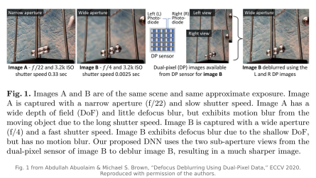
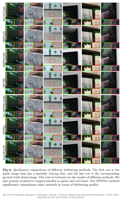
And the matte itself is the battleground, because the silhouette is rarely a clean line. Hair, fur, foliage, and glass defeat a hard binary mask (a strand of wind-blown hair is half subject, half background within a single pixel) so portrait modes lean on alpha matting: a soft, fractional foreground coverage per pixel that lets the blur blend partially through wisps of hair. Abuolaim & Brown's 2020 work on defocus from dual-pixel data Abuolaim & Brown 2020 is instructive here, using dual-pixel measurements for defocus deblurring. It illustrates the value of that extra measurement, rather than establishing that depth estimation alone solves matting. Even so, alpha matting is hard, and it leaves residue, which is the cue for the examples below.

23.2.6 Failure modes🔗⧉

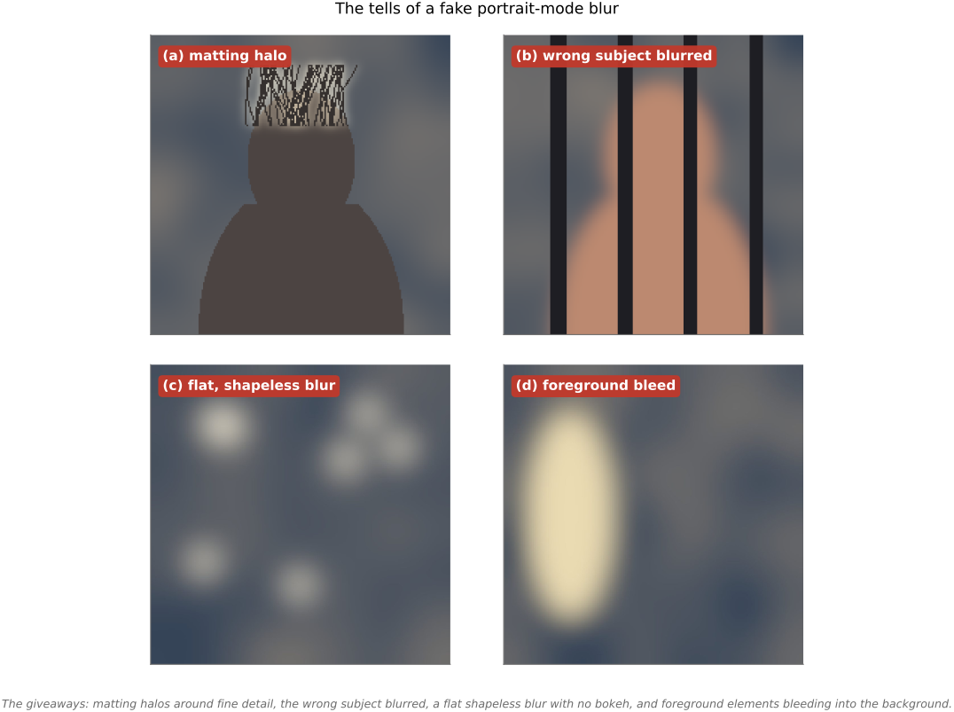
The common failure modes are easy to recognize once you know what to look for (Figure 23.2.8⛶ fullscreen). The first is the edge halo: a matting error around fine, high-frequency boundaries (wind-blown hair, a frizzy sweater, backlit foliage) where the matte cannot decide subject from background and leaves either a soft halo of background bleeding into the subject or a fringe of sharp subject stranded in the blur. The second is the flat, shapeless blur: a kernel whose profile does not match the intended pupil, compounded by lost highlight radiance in a clipped input, so the background looks smeared rather than defocused. The third is the wrong subject (the segmentation grabs the railing instead of the person, or sharpens the coffee cup and blurs the face), a depth/segmentation failure that no amount of pretty bokeh can rescue. The fourth is foreground bleed: a sharp hand or shoulder closer than the focal plane gets softened into the background because the estimated defocus magnitude or subject matte is wrong; foreground defocus itself is physically legitimate.

The chapter's main point is simple: portrait mode is a depth-estimation + matting + plausible-blur stack, and a composited result is only as good as its weakest stage, which in practice is usually the matte at fine edges. The depth-to-blur circle follows an idealized model; the bokeh can be made gorgeous; but a single misjudged strand of hair or a railing mistaken for a subject undoes all of it, because the eye polices silhouettes ruthlessly. This is the deepest lesson of the chapter, and it generalizes far beyond portrait mode to every composited, multi-stage computational image: the picture inherits the failures of its frailest component.