34.5 Single-photon sensors (SPAD, avalanche, photon counting)🔗⧉

Every sensor so far has been an integrator: it lets photons pile electrons into a well for the length of the exposure, then reads the total once. That design is effective over a wide range of light levels, but can become read-noise-limited in very dim light, where the handful of electrons a pixel manages to collect is swamped by the read noise the amplifier adds at the end (Chapter 2.8, Noise, signal-to-noise ratio and dynamic range). The single-photon sensor takes the opposite stance. Instead of waiting to the end and reading a faint total through a noisy amplifier, it amplifies each photon at the instant it lands, internally, until that one photon makes a signal so large it can be counted digitally, like a Geiger counter for light. Once you can register a single photon, two capabilities become available, depending on the readout: counting sparse detections with negligible read noise, and timing individual detections with picosecond-scale precision. Low-noise integrating sensors can also detect very weak light; they generally do not timestamp each photoelectron. That timing is the door to LiDAR, fluorescence lifetime, and looking around corners.

34.5.1 From avalanche gain to a single-photon click🔗⧉

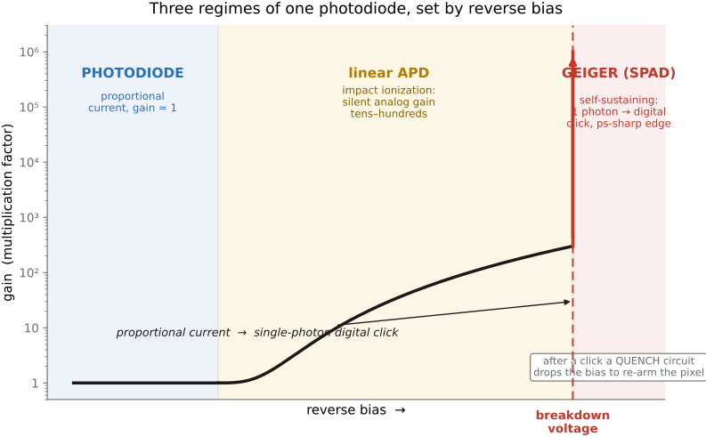
Start with an ordinary photodiode and run it in reverse bias: a photon frees an electron–hole pair, and the field sweeps them apart to make a tiny current. Now crank the reverse bias high. The freed electron is accelerated so hard between collisions that it knocks loose additional electrons on impact, which are themselves accelerated and knock loose more, a chain reaction called impact ionization, or an avalanche. One absorbed photon now yields not one electron but tens or hundreds. This is the avalanche photodiode (APD): a photodiode with built-in stochastic analog gain, exactly the trick that lets the read noise added afterward become negligible next to the (now amplified) signal. Avalanche multiplication itself adds excess noise because the gain fluctuates. APDs have long carried fiber-optic receivers and laser rangefinders for this reason.

Push the bias higher still, past the diode's breakdown voltage, and the behavior changes in kind, not just degree. Now a single electron–hole pair triggers an avalanche that is self-sustaining: it does not settle to a proportional current but runs away to a large, easily-detectable pulse, the same way a Geiger tube discharges from a single ionizing particle. This is Geiger mode, and a diode run this way is a single-photon avalanche diode (SPAD). The output is no longer an analog brightness. It is a digital click: one detected avalanche trigger, one pulse, with a rising edge so fast it pins the photon's arrival time to tens of picoseconds. Because the avalanche must then be stopped before the next photon can be seen, every SPAD has a quenching circuit that yanks the bias below breakdown to extinguish the discharge and re-arm the pixel.

34.5.2 Photon-counting arrays: zero read noise, shot-noise-limited🔗⧉

Tile SPADs into a two-dimensional array, give each pixel a quench circuit and a counter, and you have a photon-counting image sensor. Once an avalanche reliably crosses the detection threshold, the count has essentially no conventional analog read noise. Independent detected photons contribute Poisson shot noise, with standard deviation $\sqrt{N}$ for mean count $N$ (Chapter 2.8, Noise, signal-to-noise ratio and dynamic range). Real sensors also have finite photon-detection efficiency, dark counts, afterpulsing, crosstalk, and dead time. They approach the shot-noise limit only when these effects are negligible or adequately modeled; single-photon sensitivity does not make every faint-light measurement photon-noise-limited. Detector choice in astronomy and microscopy also depends on wavelength, field size, and integration time, so conventional low-noise arrays remain important.

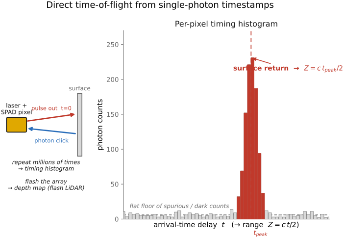
The second capability is timing. When a SPAD is connected to timing circuitry, it can mark when a detected avalanche occurred, not just how many, an array of them is a per-pixel stopwatch. Pulse a laser at the scene, and for each pixel record the delay between the outgoing pulse and the returning photon's click: that delay, times the speed of light over two, is the distance to whatever that pixel sees. This is direct time-of-flight (ToF) ranging, the principle of LiDAR, and a SPAD does it one photon at a time. A single photon is too noisy to trust (it might be a stray from the sun, or a dark count), so the trick is to repeat the laser pulse millions of times and build a histogram of arrival times per pixel; the true return shows up as a sharp peak riding on a flat background of spurious counts, and its position gives the range (Figure 34.5.2⛶ fullscreen). Flash the whole scene at once and read every pixel's histogram and you get a depth map, flash LiDAR, directly, in the dark, at the speed of a single laser burst.

The same timing ability, pointed at different physics, gives a small family of measurements that conventional intensity frames do not directly provide. Gated or modulated integrating detectors can also make some time-resolved measurements. In fluorescence-lifetime imaging microscopy (FLIM), a pulsed laser excites a fluorescent molecule and the SPAD measures the exponential decay time of the re-emitted photons, over a few nanoseconds, which reports on the molecule's chemical environment independently of how bright it is. In transient imaging and non-line-of-sight (NLOS) imaging, one records the full time-history of light scattering through a scene; the picosecond timing of indirect, multiply-bounced returns carries enough information to reconstruct geometry the camera cannot directly see, allowing it to look around a corner (Velten et al. (transient/NLOS); developed in Part 38, Revealing the invisible and Chapter 34.10, Ultra High speed Imaging). All of these are the same hardware capability, count one photon and know exactly when it came, aimed at a different question.

34.5.3 The Quanta Image Sensor: a different road to one photon🔗⧉

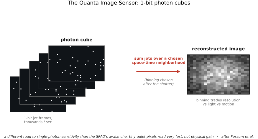
A SPAD reaches single-photon sensitivity by amplifying each photon with an avalanche. Eric Fossum, the inventor of the CMOS active-pixel sensor, proposed a different route that needs no avalanche at all: the Quanta Image Sensor (QIS) Fossum et al. (QIS). Make pixels tiny (sub-micron specks Fossum calls jots) and fast, and engineer the readout to be quiet enough that a single photo-electron clears the noise. In the single-bit version, each jot reports one bit per readout: did a photon land here in this interval, or not? Read the whole array thousands of times per second and you accumulate a photon cube, a stack of mostly-empty 1-bit frames, sparse specks of light against black (Figure 34.5.3⛶ fullscreen). An image is reconstructed from that cube by summing jots over space and time, with the freedom to choose the spatial and temporal binning after capture, trading resolution against light and motion, computationally, from one raw stream.

Multi-bit QIS devices also resolve several photoelectrons per read. In a one-bit jot, two or more photoelectrons still produce one occupied bin; summing bits approximates photon count only at low occupancy, and brighter measurements need an occupancy model. Contrast QIS with the SPAD it competes with. A SPAD gets its single-photon sensitivity from physics (avalanche gain) at the cost of a complex high-voltage, quench-per-pixel circuit and a poor fill factor; QIS gets it from engineering (tiny low-capacitance jots and very quiet, very fast readout) in an almost ordinary CMOS process, at the cost of an enormous data rate of 1-bit frames to move and reconstruct. Both deliver the same result, a sensor where every photon counts, and both relocate the burden from the analog noise floor to the computation that turns sparse photon events into a picture.

34.5.4 What it costs: dark counts, dead time, fill factor, data rate🔗⧉

Single-photon sensitivity is not free, and the price is a set of artifacts that are the mirror image of an integrator's. The main ones to know:

• Dark counts. A thermally-freed electron triggers the same avalanche a photon does, so a SPAD clicks even in total darkness. The dark-count rate is the single-photon version of dark current (the thermal noise of Chapter 2.8, Noise, signal-to-noise ratio and dynamic range): a floor of false photons that cooling suppresses and that the ToF histogram's flat background is made of.
• Dead time and pile-up. After each click the pixel is dead while it quenches and re-arms, over tens of nanoseconds, during which it is blind. If photons arrive faster than the pixel can recover, later ones are missed, so the measured count saturates below the true rate. Worse for timing: the pixel preferentially registers early photons in each cycle and misses the ones behind them, biasing a ToF histogram toward shorter delays, the classic pile-up distortion, corrected by keeping the flux low (≲5% detection per pulse) or by modeling it.
• Afterpulsing and crosstalk. Trapped carriers can trigger a later avalanche in the same detector, and avalanche light or electrical coupling can trigger neighbors. These correlated false events violate a simple independent-Poisson model.
• Fill factor. The quench and timing circuitry crowds the active area, so a SPAD pixel collects light over a smaller fraction of its footprint than a plain photodiode, giving a low fill factor that microlenses and back-illuminated, wafer-stacked designs (compute under the pixels) only partly recover.
• Data rate. Timestamping every photon, or reading a jot array thousands of times a second, generates a torrent of raw data, in the gigabits per second, that must be moved and reduced on-chip. The frontier of these sensors is as much a readout and compute problem as a photonics one.

An ordinary sensor's dynamic range is bounded at the top by full-well capacity, the most electrons a pixel can hold before it saturates (Chapter 2.8, Noise, signal-to-noise ratio and dynamic range), and runs out of room in bright light. A single-photon sensor is bounded the opposite way: it can register individual detections, so it reaches into near-total darkness, but dead time and pile-up cap it from above, in bright light, where photons crowd faster than it can count them. The two technologies are tuned to opposite ends of the same axis, which is why a complete computational camera may want both, and why Chapter 34.8, Specialized and research sensors and the LiDAR systems of the next sections pair single-photon detectors with conventional imagers. Like Chapter 34.7, Event sensors of a later section, a timestamping SPAD can report asynchronous detections of light itself. Other SPAD arrays output framewise counts or histograms, and QIS commonly outputs synchronous bit planes. The measurement differs from an event camera, where the event sensor reports a change in brightness.