8.11 File formats and compression⧉
An image file stores pixel values together with enough structure to decode them, and often metadata about color and capture. At this boundary, check orientation, channel order, bit depth, color interpretation, and compression. A correctly decoded array can still be misinterpreted or carry artifacts from earlier processing.
Compression exploits predictable data, and lossy photographic compression also exploits visual tolerance. JPEG makes these choices concrete: separate luma and chroma, transform local structure into coefficients, quantize, then encode the remaining symbols. The savings and the visible errors depend on image content and viewing conditions.
JPEG is useful here because it makes perceptual design concrete. Separate controls for chroma resolution and spatial-frequency quantization turn observations about vision into adjustable numerical choices. They can be tested against file size and visible error. Perception does not determine one universally correct table, but it supplies engineering constraints that can be measured and compared.
8.11.1 The big picture: none, lossless, lossy⧉
Storing an image costs bits, and there are exactly three philosophies about how to spend them.
The first is to write the pixels directly, one number after another, and read them back the same way. This is uncompressed storage: a plain dump of the array. It is simple, exact, and fast, but it is large: a 12-megapixel photo at 8 bits per channel is roughly 36 megabytes, and a folder of them fills a disk in a hurry. This is what a memory-resident image, or a no-frills format, amounts to.
The second philosophy is lossless compression: shrink the file, but promise that what comes back out is bit-for-bit identical to what went in. This is possible because real images are not random noise. Neighboring pixels tend to be similar, large regions are nearly constant, edges repeat, and that statistical redundancy can be squeezed out and then perfectly restored, the way a ZIP archive shrinks text without losing a character. PNG and (usually) TIFF live here. Lossless is the right call when every pixel is sacred: a mask, a depth map, scientific data, or an image you will edit and re-save many times.
Lossy compression permits decoded samples to differ from the input in exchange for a smaller file. JPEG commonly uses this approach. HEIF, WebP, AVIF, and JPEG XL support different codecs or modes, including lossless options; the extension alone does not establish whether information was discarded. Keep a suitable master when later editing or measurement matters.
Lossless compression preserves the samples presented to the codec. It cannot undo an earlier conversion to a palette, a lower bit depth, or another color space. Lossy compression can trade exact reconstruction for rate, using visual quality or another task-specific objective.
8.11.2 Data versus metadata: EXIF⧉
Image metadata describes dimensions, sample types, orientation, and color interpretation. Filesystem properties such as path and modification time are separate and can change when a file is copied. Capture metadata records how and when the image was made; it is not part of the pixel array.
Cameras write a far richer layer of capture metadata into a standardized block, the exchangeable image file format (EXIF), a set of tagged fields stored alongside the pixels. This is where you find the ISO, shutter speed, aperture, and focal length the photo was taken at, along with the lens model, whether the flash fired, a timestamp, and often a Global Positioning System (GPS) location. For a computational photographer it is the physical record of the shot, and later chapters on exposure and noise read these fields directly; for a photo library it is what sorts by date, plots shots on a map, or auto-rotates a sideways frame. GPS is the double edge: handy for organizing a library, and a real privacy concern when you post a file without thinking. Sorted by capture time, years of phone photographs become a detailed diary: you can watch children grow frame by frame, or find exactly where you stood and which lens you used on a trip a decade ago. The same fields can pinpoint your home in a file posted straight from the camera; exiftool reads and strips them.
The quickest way to see what that block actually holds is to open one of your own files and look (Figure 8.11.1).
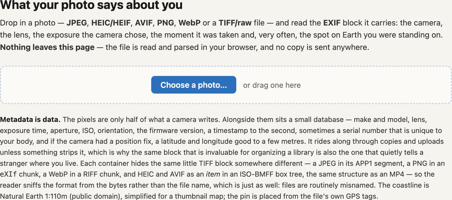
Treat EXIF as a hint, not a measurement: two things go wrong. First, coverage is incomplete and inconsistent, not every camera writes every field, and the exact set and formatting differ from maker to maker, so any code that reads EXIF has to tolerate missing and oddly-encoded values. Second, and more dangerous, some numbers are only approximate. The recorded ISO and shutter speed in particular are routinely rounded to tidy nominal labels and are not radiometrically correct: they will not let you reconstruct the true exposure, or compare two frames' light, to the precision the digits imply. Do not treat EXIF capture values as calibrated measurements.
Orientation can include mirroring as well as rotation. Determine whether the decoder already applied it; apply it once, and update or remove the tag when saving transformed pixels. Color interpretation is separate: ICC profiles are not simply EXIF fields and can describe more than primaries plus a gamma. A color-managed conversion uses the source and destination profiles; embedding a profile alone does not ensure identical appearance on every display.
A recurring wish in this book: beyond the basics above, a sane image representation would carry exactly the things a bare array can never imply on its own:
- the encoding (linear / gamma / log, the very ambiguity Chapter 8.2, What the numbers mean is about);
- the color space / primaries, ideally as an embedded ICC profile;
- the noise level (the read- and shot-noise parameters) so downstream code knows the per-pixel uncertainty it is working with;
- and, when it is known, the point spread function (PSF), the blur the optics imposed, which is exactly what Chapter 6.3, Fourier needs to undo it.
Metadata support varies: DNG, for example, can carry a noise profile. Such metadata must be updated when processing changes the values and their uncertainty. Yet the algorithms that come later silently need this provenance: white balance and HDR want the encoding and color space, denoising wants the noise parameters (see edge-preserving filtering), deblurring wants the PSF. The plain view, then, is that an image is its pixels plus this provenance, and a representation that drops it forces every later stage to guess.
Capture dates, locations, and camera settings can make a library easier to search. Fields may be absent or wrong. Inspect location and identifying metadata before sharing a file; Chapter 45.13, EXIF and image metadata describes typical fields.
8.11.3 PNG: the format we read from⧉
PNG is convenient for exercises because its compression preserves the stored samples exactly. It supports grayscale, palette, and RGB images, optional transparency, and integer sample depths up to 16 bits. Saving a floating-point array as an 8-bit PNG still requires a potentially lossy conversion before compression.
PNG filters scanlines to form predictable residual bytes, then compresses them with DEFLATE. Inspect the decoded shape and dtype: a library may expand palette indices, add alpha, or return grayscale. If transparency is unwanted, decide whether to discard alpha or composite against a chosen background; those operations produce different RGB images.
In practice you never touch the PNG bitstream yourself; a library does it in one call.
import imageio.v3 as iio
img = iio.imread("input.png")      # an (H, W, 3) , or (H, W, 4)! , array
iio.imwrite("output.png", img)
The whole point of a standard format is that this line just works. Mind the dtype the library hands back (usually 8-bit uint8 in [0, 255], which we convert to float [0, 1]) and the channel count.
8.11.4 JPEG: compression by perception⧉
The common baseline JPEG path Wallace 1991 combines lossy quantization with lossless entropy coding. Color conversion and optional subsampling commonly precede the block codec. JPEG also specifies modes beyond this baseline; the following description concerns the usual 8-bit photographic workflow.
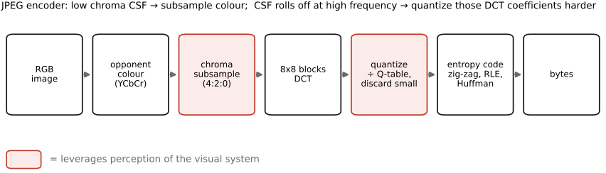
Y from two chroma channels Cb, Cr. (2) Chroma subsampling: shrink Cb and Cr to half resolution (4:2:0), exploiting the eye's low color acuity. (3) Block DCT: split each channel into 8×8 blocks and transform each to spatial-frequency coefficients. (4) Quantization: divide the coefficients by a quality-dependent table that crushes high frequencies hardest; this is the only lossy step. (5) Entropy coding: losslessly pack the (mostly zero) quantized coefficients in a smart order. Decoding runs the same chain in reverse.The starting observation, lifted straight from Chapter 3.4, Spatial and temporal vision, is that human vision is not uniform. The contrast sensitivity function (CSF) tells us our sensitivity to detail falls off at high spatial frequencies: we simply cannot resolve fine texture as well as coarse structure. And our sensitivity to color detail is far lower still than our sensitivity to brightness detail: the eye has sharp acuity for luminance and surprisingly coarse acuity for hue. JPEG's entire strategy is to match the number of bits to what the eye can actually use: many bits for the brightness structure we see keenly, few for the color detail and the high frequencies we barely register. The five stages below implement that allocation.
Stage 1: opponent color⧉
A common color JPEG converts encoded RGB to $Y'CbCr$. The weighted sum $Y'$ is luma, while $Cb$ and $Cr$ represent scaled blue-minus-luma and red-minus-luma differences. This provides separate controls over brightness-like and chromatic information. It is not the retina's exact opponent transform. The ideal affine transform is invertible; finite-precision conversion and clipping can introduce small losses.
The transformed RGB gamut occupies only part of the nominal $Y'CbCr$ box. Values outside that region are outside the original RGB gamut, not necessarily physically impossible colors. Code-range occupancy depends on the transform and range convention, so a universal percentage is misleading.
We follow one 32×32 image through all five stages of Figure 8.11.3, starting with this conversion (stage color).
Y′ and the chroma differences Cb and Cr, each drawn in gray, where 128 means no chroma. Below: the selected 8×8 region of each plane as numbers, and the selected pixel's conversion with the JFIF coefficients before and after rounding to 8 bits. Click any plane or any cell to move the pixel; the menu picks the input, four crops of photographs from this chapter and two synthetic images. The red hibiscus is bright in Cr and nearly flat in Cb; the red disk on teal is drawn at almost the same luma as its background, so its edge nearly vanishes from Y′. Rounding the planes to 8 bits already costs a little: R′G′B′ rebuilt from them measures about 53 dB PSNR. Photographs: Frédo Durand.Stage 2: chroma subsampling⧉
With color now isolated in Cb and Cr, JPEG makes its first lossy reduction, with little perceptual cost. Because our acuity for color detail is so low, JPEG simply throws away half or three-quarters of the color resolution: it shrinks the two chroma channels while keeping luma at full resolution. This is chroma subsampling, written in a J:a:b notation that counts how many chroma samples survive in a $4\times2$ block of pixels (Figure 8.11.4). 4:4:4 keeps full color resolution (no subsampling at all). 4:2:2 halves the horizontal color resolution. 4:2:0, the usual JPEG choice, halves it in both directions (one color sample for every $2\times2$ block of luma, a 75% cut in color data) and visibility depends on the image and viewing scale.
Lower chromatic acuity often makes chroma subsampling acceptable for photographs. It can be conspicuous on colored text, saturated edges, and fine color patterns. Low-pass filter before decimation and specify chroma sample positions; simply dropping samples aliases, and inconsistent siting shifts color boundaries.
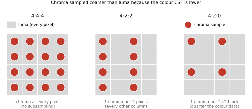
Cb and Cr (full color resolution). 4:2:2: chroma sampled every other column (half the horizontal color resolution). 4:2:0 (JPEG's usual choice): one chroma sample per 2×2 block, color resolution halved in both directions, a 75% reduction. Luma (Y) is always kept at full resolution. Because the eye's color acuity is low, even 4:2:0 is nearly invisible; try the same on luma and edges smear.Figure 8.11.5 compares luma and chroma coarsening on a photograph. Inspect saturated boundaries as well as ordinary texture. Full-resolution luma cannot preserve an isoluminant color edge whose structure lies entirely in chroma.
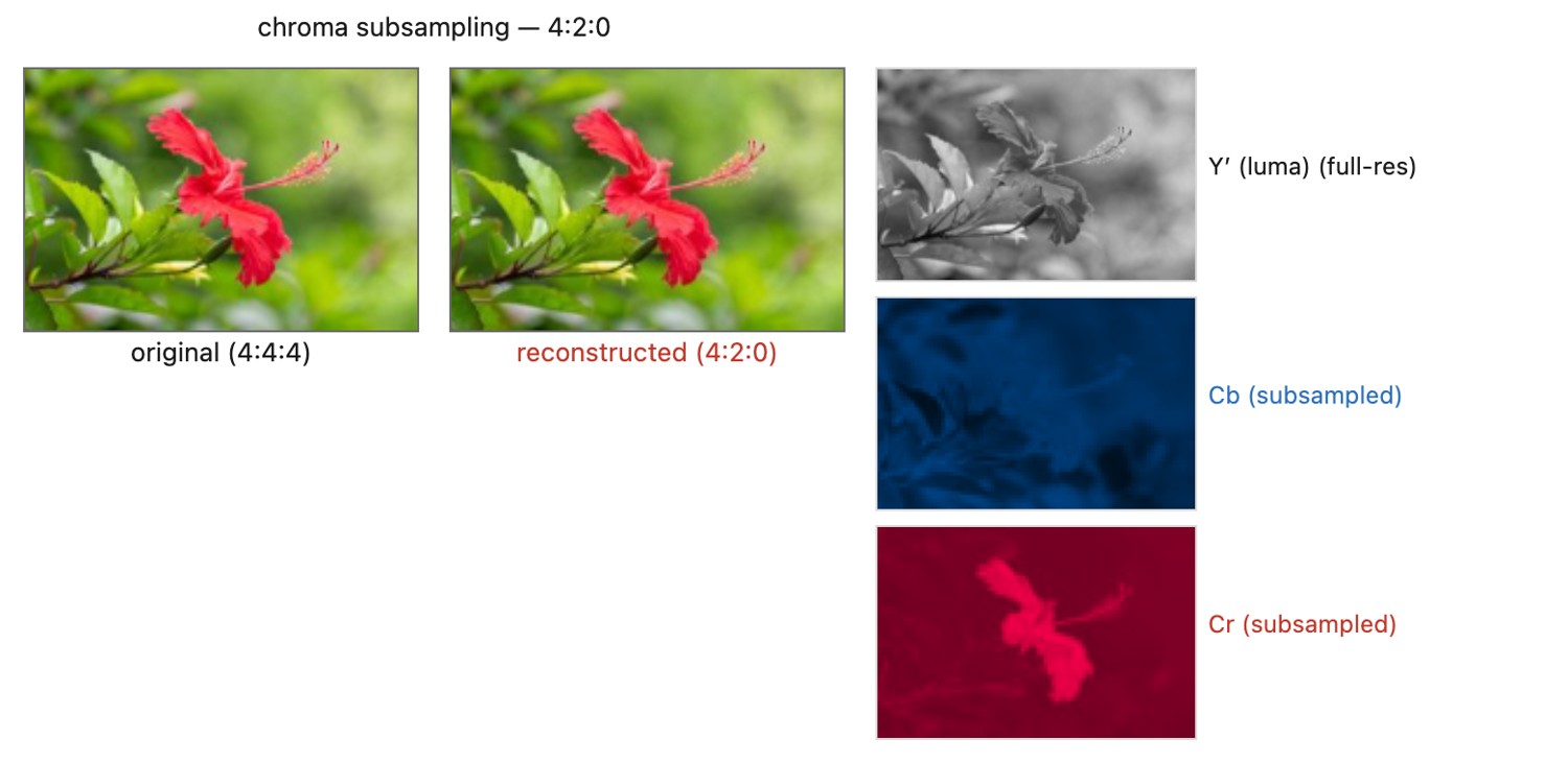
Y′ holds every contour. Right, the Y′, Cb, and Cr planes, so you can watch which one is coarsened. Now flip coarsen to luma: the same block-averaging applied to Y′ instead smears every edge and the image falls apart. The perceptual bet behind chroma subsampling, made visible: resolution belongs in luma, never chroma.On the small image of Figure 8.11.3, stage subsample, the same step removes three quarters of the chroma samples. It is also the only loss left at the top of the quality scale: at quality 100, on every input of the figure, the decoded image is exactly as far from the original as 4:2:0 subsampling alone makes it.
Cb and Cr planes in the strip are now 16×16: each sample is the average of a 2×2 cell of the full-resolution plane, shown below as numbers for the selected 8×8 region, with the arithmetic for the selected cell. Top right, the image rebuilt from full-resolution Y′ and the 4:2:0 chroma upsampled with libjpeg's triangle filter. The image keeps 1,536 of its 3,072 samples. On crops this small, each pixel stands for many pixels of the photograph, so the loss is larger than on a full-size image: the rebuilt hibiscus measures 26.3 dB PSNR, the egret 31.8 dB, and the red disk on teal 19.9 dB, because its edge and its one-pixel line live only in chroma and spread over their neighbors.Stage 3: the 8×8 DCT⧉
Now JPEG turns to the high-frequency half of the CSF story, and to do that it must work in terms of spatial frequency rather than raw pixels. It splits each channel into small $8\times8$ pixel blocks and transforms each block with the discrete cosine transform (DCT). The DCT is a close relative of the Fourier transform we study in Chapter 6.3, Fourier: it re-expresses the 64 pixel values of a block as 64 coefficients, each the weight of a particular 2-D cosine basis pattern, from a flat constant (the block's constant component, the "DC" term), through gentle ramps, up to fine checkerboards at the highest frequencies (Figure 8.11.6). No information is lost yet; the DCT is just a change of representation, perfectly invertible, like rewriting the same number in a different base.
For a level-shifted block $b_{xy}$ (subtract 128 for 8-bit input), an orthonormal convention is
with $\alpha_0=1/\sqrt8$ and $\alpha_k=1/2$ for $k>0$. Then $C_{00}=8\,\operatorname{mean}(b)$, not the mean itself. For positive table entries $Q_{uv}$,
The ideal coefficient error is bounded by $Q_{uv}/2$, subject to the rounding convention. Integer DCT implementations can add numerical differences.
Why bother? Because frequency is exactly the axis the CSF is organized along. Once a block is expressed as frequency coefficients, JPEG can treat low and high frequencies differently: keep the coarse structure the eye sees keenly, crush the fine detail it barely registers. And there is a statistical bonus: on real photographs, most of a block's energy piles into the low-frequency coefficients (smooth regions dominate), so the high-frequency coefficients are usually small to begin with. The DCT thus concentrates the signal into a few coefficients, which is what makes the next two stages so devastatingly effective. (Why $8\times8$ and not the whole image? A small block keeps the transform cheap and lets the encoder adapt to local content, but it is also the source of JPEG's signature artifacts, as we will see.)
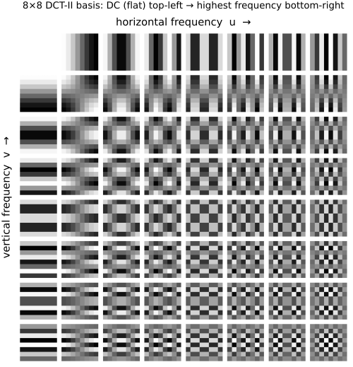
Figure 8.11.3, stage dct, applies the transform to one block of the small image. On a block of a petal, the six lowest-frequency coefficients hold 77% of the block's energy; on a smooth ramp, more than 99%.
Y′ in the strip, or of the 16×16 Cb or Cr plane, to transform that one instead. On the hibiscus petal block selected at first, the six lowest coefficients hold 77% of the energy; on the smooth ramp, more than 99%.Stage 4: quantization, the lossy step⧉
This is another stage where JPEG throws information away, and where its quality knob lives. Each of the 64 DCT coefficients is divided by a corresponding entry in a quantization table and rounded to the nearest integer. The rounding is the lossy act: once you have rounded 7.4 to 7, you cannot recover the original: that fractional detail is gone forever. The quantization table decides which coefficients to round coarsely and which to keep fine.
Quantization tables usually assign larger steps to high-frequency and chroma coefficients. Perceptual sensitivity motivates that allocation, but a table is not a direct universal measurement of the CSF. Image statistics, display size, viewing distance, and encoder design also matter.
An encoder's quality setting commonly scales quantization tables, and may also change subsampling or other decisions. Quality numbers are not standardized across encoders. The decoder reads the actual tables from the file; it multiplies quantized integers by those entries before the inverse transform.
An orthonormal DCT preserves total squared error. If pixel rounding errors were independent with equal variance, their coefficient errors would have equal variance too. A single quantized basis pattern does not satisfy that statistical assumption in general: deterministic rounding, clipping, basis normalization, and amplitude affect the result. Thus an 8-bit block does not guarantee eight useful bits in every individual coefficient.
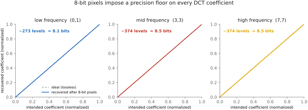
The DCT rounding experiment separates two reasons a high-frequency coefficient may be small or imprecise. Pixel quantization limits the input measurements; JPEG’s coefficient quantization makes a further, deliberate allocation of error. Under an independent equal-variance rounding-noise model, an orthonormal transform does not inherently make its high-frequency coordinates noisier than its low-frequency ones. Coarser high-frequency quantization is therefore a coding choice motivated by statistics and visibility, not a requirement that a pixel array can only represent low frequencies.
Figure 8.11.3, stage quantize, quantizes that block at a quality we choose.
Stage 5: entropy coding⧉
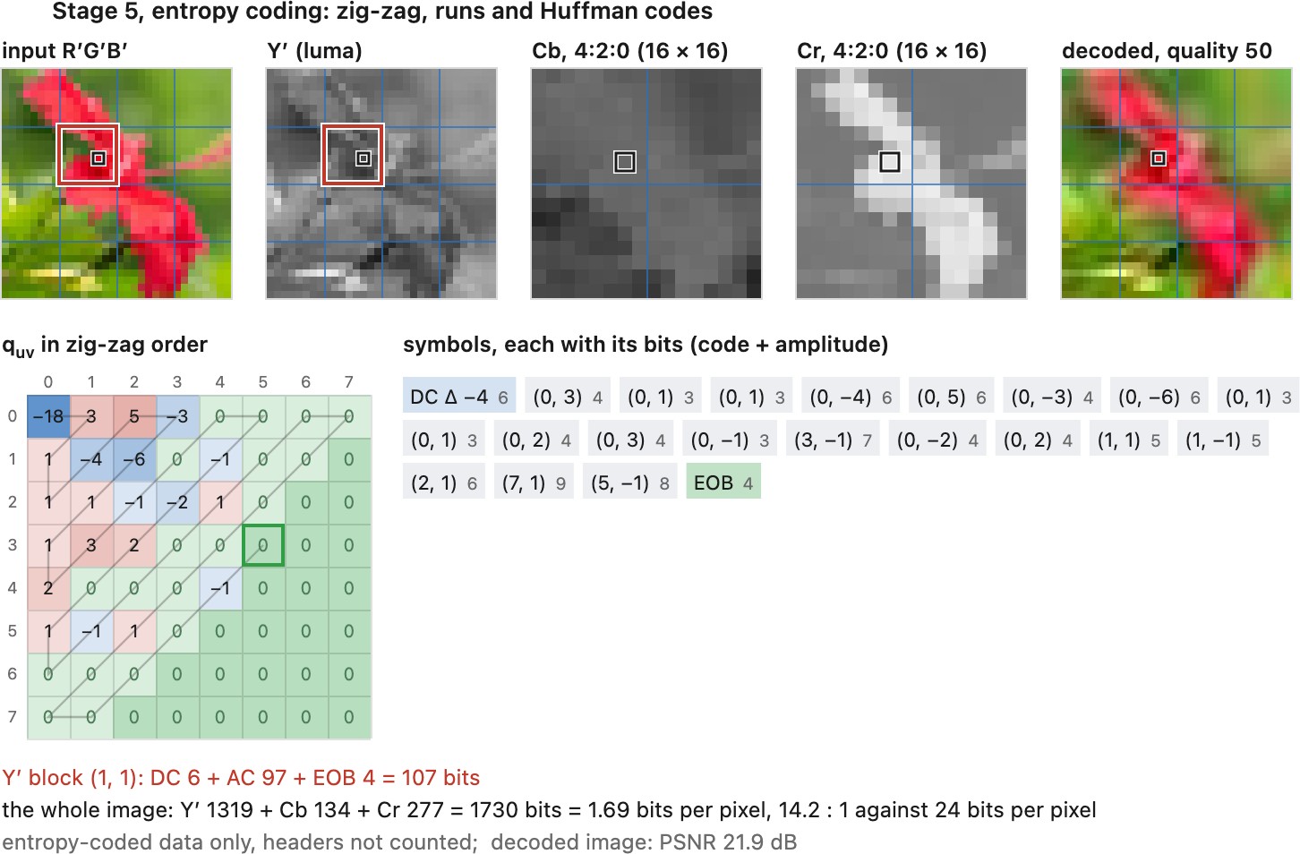
In baseline JPEG, the DC coefficient is coded as a difference from the preceding block's DC in that component. AC coefficients are scanned in zig-zag order; run lengths describe zeros before a nonzero value, and an end-of-block symbol omits trailing zeros. Huffman codes pack these symbols, with additional bits for coefficient amplitudes. This stage is lossless with respect to the quantized integers. Decoding reconstructs those integers, dequantizes, applies the inverse DCT, and performs the necessary color upsampling and conversion.
The transform and scan order prepare the data for lossless coding. After quantization, many high-frequency AC coefficients are zero. Scanning roughly from lower to higher frequencies tends to move long zero runs toward the end of the sequence, where an end-of-block symbol can replace them. Neighboring blocks also often have similar averages, which makes differences between DC coefficients economical to encode. The entropy coder benefits from this predictable structure. It cannot restore information already removed by quantization, but it need not lose anything more.
Figure 8.11.3, stage entropy, counts the bits of the small image symbol by symbol. At this size the coded scan is only a small part of a real file: at quality 50 the hibiscus crop takes 843 bytes, 626 of them headers and tables, so the file is about 3.6 times smaller than the raw pixels while the scan alone is 14 times smaller. Compression ratios quoted for JPEG assume images large enough for that fixed overhead not to matter.
JPEG combines optional chroma subsampling and coefficient quantization with lossless coding. Perception helps allocate the loss, while signal statistics help encode what remains. Neither the transform nor entropy coding alone produces the large lossy savings.
Limitations and artifacts⧉
Baseline JPEG stores 8-bit component samples and can visibly block or ring at strong compression. Neither the file extension nor a high quality setting supplies the precision and scene-referred latitude of a suitable raw or floating-point master.
The two familiar artifacts come from different aspects of the representation. Each 8×8 block has its own quantized coefficients. Neighboring blocks can reconstruct different values at their shared boundary, revealing the block grid. Within a block, a sharp edge needs several spatial-frequency components; changing those components can create ripples near the edge. Sharpening the decoded image can amplify both the block discontinuities and the ripples.
Different decoders can differ in IDCT rounding, chroma upsampling, color management, and optional enhancement. Record those choices when exact decoded pixels matter. Repeated save/load behavior cannot be attributed to deblocking without checking what the application actually does.
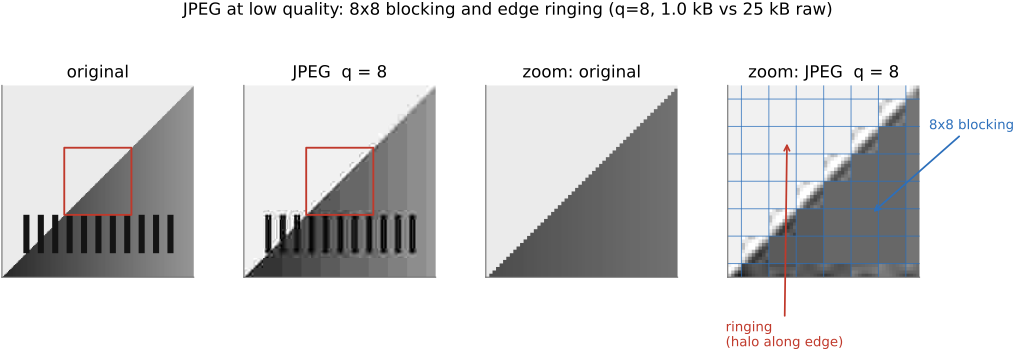
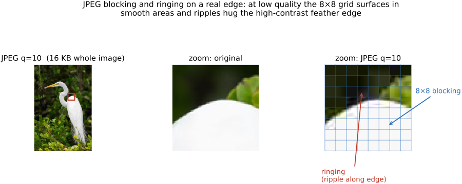
The clean test edge of Figure 8.11.8 isolates the two artifacts; Figure 8.11.9 shows them where you actually meet them: on a real photographic edge. Save a photo with a hard, high-contrast boundary (a white egret against dark foliage) at low quality, zoom in, and overlay the encoder's $8\times8$ grid: the grid surfaces as flat seams across the smooth bright region (blocking), and faint ripples cling to the high-contrast edge (ringing). These are exactly the fingerprints a careless sharpening filter will then magnify.
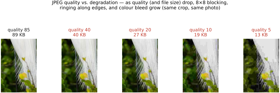
The trade-off is clearest as a sweep (Figure 8.11.10): save the same photo across a range of quality settings and watch the file size and the damage move together. The file shrinks several-fold, and the degradation marches in step: near-invisible at high quality, a softening of fine detail through the middle, then unmistakable blocking and color bleed at the bottom. This is the tradeoff behind the quality slider: the same knob trades measurable bits against just-noticeable damage.
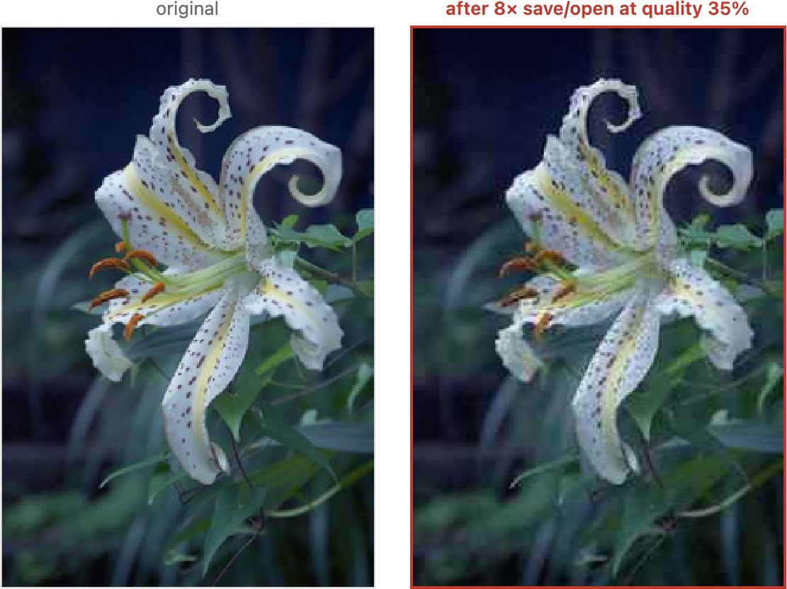
Repeated decoding and encoding can change an image, but the error need not grow at a fixed rate or monotonically. Some unchanged settings and codecs settle quickly; other combinations drift or cycle. Color conversion, subsampling, rounding, edits, and block-grid shifts all affect the loop. Keeping a master and exporting from it avoids relying on such stability.
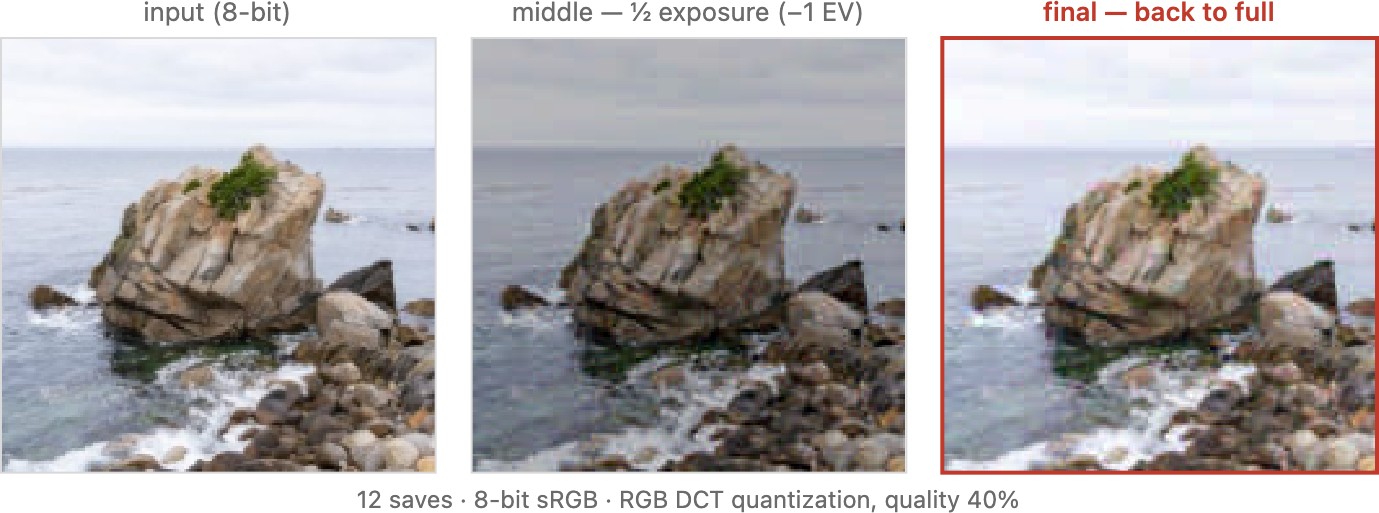
Editing between saves changes the samples being quantized. Darkening and brightening through an 8-bit JPEG adds both sample rounding and coefficient quantization. Compare the final result with an edit performed at higher precision followed by one export.
A fixed coefficient quantizer is idempotent on its own reconstruction levels. A full decode/edit/encode pipeline includes other operations, so that property does not prove that the whole loop converges. Even a deterministic finite-state loop can enter a cycle.
The cited re-save experiment Krawetz, "How I Met Your Mother Through Photoshop" illustrates application-dependent drift. It does not by itself identify which processing step caused the drift; that requires the software version, settings, and decoder behavior.
Use these demonstrations to inspect a particular codec loop, rather than as proof that all JPEG round-trips converge or that all drift comes from deblocking.
The format therefore affects how a later filter should be evaluated. A denoiser or sharpener applied to a camera JPEG is processing existing compression artifacts along with scene detail and sensor noise. Keep a lossless intermediate while developing a chain of edits so additional lossy encoding does not obscure which stage introduced an artifact.
Removing the artifacts: JPEG deblocking⧉
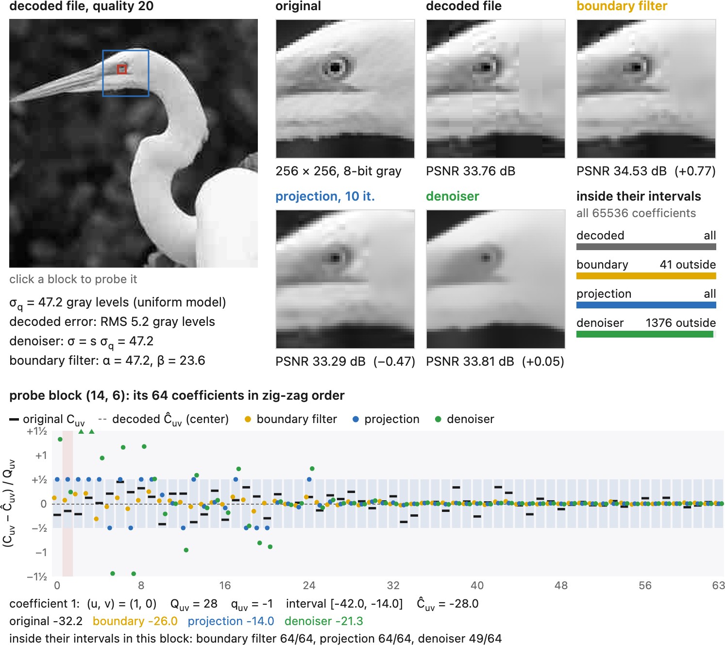
A decoder that only inverts the DCT shows the blocks and the ringing. Deblocking, or compression-artifact reduction, estimates a cleaner image from the same file. It has more to work with than an ordinary denoiser, because it knows exactly how the image was damaged. The file stores the quantization table, so for every block we know each integer coefficient $q_{uv}$ and its step $Q_{uv}$. The original coefficient was rounded to $\hat C_{uv}=Q_{uv}\,q_{uv}$, so it lay somewhere in the interval
Every image whose block DCTs fall inside these intervals would have produced the same file. The standard decoder picks the center of every interval, which is the one choice that ignores what images look like. Deblocking picks, among all the images consistent with the file, one that looks more like a photograph. The intervals form a convex set, the quantization constraint set, and the methods differ in the image model they use to choose inside it.
Filtering the block boundaries. The simplest methods smooth across the 8×8 grid only. A step between two blocks is suspicious when it is small compared with the quantization step, because quantization can create a step of that size from nothing; a large step is more likely a real edge and is left alone. Video codecs build this decision into the decoder: H.264 filters each block edge with a strength set by the quantization parameter and by thresholds on the steps across it List et al. 2003 (H.264 deblocking). There the filter is in the loop, since filtered frames serve as references for predicting the next ones (Chapter 30.2, Video compression and motion compensation). For a JPEG it is a choice of the viewer or of a later processing step.
Projecting back onto the file. Zakhor alternated two steps Zakhor 1992 (deblocking, POCS): a low-pass filter that removes the block edges, then a projection back onto the constraint set, which takes the DCT of every block and clamps each coefficient into its interval. Clamping undoes whatever part of the smoothing the file rules out, so the result keeps every edge the file can prove and loses the block edges it cannot. Yang, Galatsanos and Katsaggelos cast the same idea as regularized reconstruction, a smoothness penalty minimized under the constraint Yang, Galatsanos & Katsaggelos 1993. Consistency with the file is not closeness to the original, though. On a smooth image the projection gains several decibels; on a textured photograph it removes the block edges but lowers PSNR slightly after its first iteration, because the low-pass pushes the coefficients that carry texture all the way to the end of their interval nearer zero, further than the original values usually were (Figure 8.11.13).
deblock(decoded, q, Q, iterations):
    x = decoded
    repeat iterations times:
        x = smooth(x)                                   # the image model
        for each 8x8 block b of x:
            C = dct8(b)
            C = clamp(C, Q * (q - 0.5), Q * (q + 0.5))   # back into the file's intervals
            b = idct8(C)
    return x
The projection is exact only for the luma channel at full resolution. Chroma was also subsampled before its DCT, and the decoded pixels were rounded and clipped to 8 bits, so a real implementation projects the chroma at its own resolution and accepts that the constraint is approximate.
Treating the error as noise. If each coefficient's error is spread evenly over its interval, its variance is $Q_{uv}^2/12$, and since the DCT is orthonormal, the average error variance per pixel is
For the standard luminance table, $\sigma_q$ is about 19 gray levels at quality 50, 10 at quality 75 and 4 at quality 90. A denoiser told this noise level can then remove the artifacts. This is an overestimate, because most high-frequency coefficients were close to zero before quantization and their errors are smaller than the uniform model says. On the photograph of Figure 8.11.13 the actual error is six to nine times smaller than $\sigma_q$, and a denoiser does best when told 0.3 to 0.5 $\sigma_q$; told $\sigma_q$, it smears detail. The error is also not like sensor noise: it is correlated within each block and aligned with the grid. Methods that adapt the shape of their support to the image, such as the shape-adaptive DCT of Foi, Katkovnik and Egiazarian, smooth inside regions without crossing edges and remove blocking and ringing together Foi, Katkovnik & Egiazarian 2007 (SA-DCT).
Learned deblocking. Training pairs are easy to make: compress clean photographs at chosen qualities and train a network to undo it. AR-CNN was an early network for this Dong et al. 2015 (AR-CNN), and DnCNN handled Gaussian denoising and JPEG deblocking with one model Zhang et al. 2017 (DnCNN). Since the file carries its quantization table, the network does not have to guess how strong the compression was. FBCNN estimates a quality factor and lets the user change it, trading artifact removal against detail Jiang, Zhang & Timofte 2021 (FBCNN). A strong network can remove real texture along with the artifacts, and one trained with a perceptual or adversarial loss can invent detail that the file does not support. Projecting the output back onto the constraint set checks the second problem: whatever remains is at least consistent with the file.
Deblocking produces an estimate, not the original. The information the quantizer removed is gone, and a deblocked JPEG is the original only in the sense that it would compress to the same file. For measurements or forensic work we keep the decoded image and the file, and state which deblocking, if any, was applied.
Figure 8.11.13 runs the first three methods side by side on one photograph and checks each against the file's intervals.
Making JPEG differentiable⧉
Rounding has zero derivative almost everywhere and is discontinuous at its thresholds. To optimize through JPEG, one can use a smooth approximation or a straight-through gradient estimate Shin & Song 2017 (DiffJPEG). A straight-through estimator changes the backward calculation, not the true derivative of rounding. Tensor implementations must also model value ranges, subsampling, and rounding conventions; validate the trained result with the actual deployment codec.
Differentiating through compression matters when training an upstream operation to survive it. Examples include a watermark that must remain detectable after JPEG, an enhancement that should not create fragile high-frequency detail, or a reconstruction network trained on compressed inputs. A surrogate backward pass can provide a useful optimization signal even though it is not the derivative of actual rounding. Evaluate the result through the real codec afterward; optimizing the surrogate alone can exploit discrepancies in the approximation.
8.11.5 RAW files: before the cooking⧉
Raw storage retains data from an earlier stage of the camera pipeline, leaving more reconstruction and rendering choices to the developer. The file may contain a CFA mosaic, demosaicked channels, or partly processed measurements. Raw capture offers latitude, but does not guarantee unmodified or losslessly stored sensor data.
To obtain scene-linear working values, decode the stored representation, apply any linearization table, subtract calibrated black levels, and use the metadata-defined scale. A linear DNG can already contain reconstructed channels. Check processing tags and profiles rather than assuming the extension establishes the numerical domain.
Here is the subtlety, stated plainly: "RAW" is not always purely raw. The name suggests an untouched sensor dump, but in practice most cameras pre-cook the data to some degree: subtracting the sensor's black level, correcting defective and hot pixels, sometimes applying lens-shading or vignetting correction or even mild denoising. Some "RAW" formats are themselves lossy-compressed or non-linearly encoded to save space. So RAW is best thought of as a spectrum of how cooked the data is, from a near-literal readout to something already partly processed, not a single guarantee of pristineness.
There is also a practical headache: RAW is largely proprietary. Nearly every manufacturer ships its own format and extension: Canon's (CR3 files), Nikon's (NEF files), Sony's (ARW files), and so on, each subtly different. That creates software and archival problems, since a format only one company supports may not be readable in thirty years. Adobe's Digital Negative (DNG) format is an open, documented, standardized RAW container meant to fix exactly this (its specification Adobe DNG specification is the reference here); many photographers convert their proprietary RAWs to DNG for safekeeping, and some cameras shoot DNG directly.
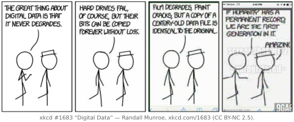
You will not parse a proprietary RAW format yourself; a library decodes the mosaic and metadata for you. The classic is dcraw, a single heroic C file that reverse-engineered dozens of formats; its maintained successor is LibRaw (C++), with a friendly Python wrapper, rawpy:
import rawpy
with rawpy.imread("photo.dng") as raw:
    bayer = raw.raw_image.copy()  # retain samples after closing raw
    pattern = raw.raw_pattern
    pattern = None if pattern is None else pattern.copy()
    rgb   = raw.postprocess()      # or let LibRaw develop it to RGB
Beyond these, open-source developers darktable and RawTherapee, Adobe's DNG Converter and DNG software development kit (SDK), and exiftool for metadata round out the toolkit; commercial Lightroom and Capture One are the mainstream developing apps.
8.11.6 HDR formats: more than 8 bits⧉
HDR storage requires an encoding that covers the intended range at adequate precision. Floating point is useful for scene-linear processing, but not required for HDR display delivery: nonlinear integer encodings such as PQ or HLG can represent HDR signals. Conversely, additional integer bits do not automatically provide values above a chosen normalized white.
OpenEXR supports half and full floating-point channels, arbitrary additional channels, and both lossless and lossy compression. Radiance RGBE uses a shared exponent per pixel; it supports nonnegative high-range RGB but loses relative precision in a small channel beside a large one. TIFF can store integer or floating-point samples, subject to reader support. Choose both the sample representation and compression mode explicitly.
A gain-map file pairs a base rendering with metadata and an auxiliary image for adapting it to another display range. An SDR JPEG base remains viewable by older software, while compatible software can reconstruct an HDR rendering. Android Ultra HDR and ISO 21496-1 have distinct metadata conventions that can coexist; compatibility depends on the writer and reader, not just the .jpg extension.
8.11.7 Modern formats⧉
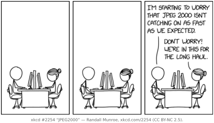
JPEG 2000 replaces the block DCT with wavelet coding, supporting reversible and irreversible paths and scalable access. It avoids baseline JPEG's fixed 8×8 blocking pattern but can still blur or ring at strong compression. Its use in specialized imaging does not imply universal application support. It found its homes where lossless modes, very large images and region-of-interest access matter more than browser support: it is the image codec of the Digital Cinema Package delivered to theaters, and common in medical (DICOM), archival, and satellite and geospatial imaging. On the web, patent uncertainty, encoder complexity and scant browser support kept it from displacing JPEG.
Modern formats add compression tools and capabilities such as alpha, animation, higher precision, or HDR. Compare the features of the chosen codec and profile with those supported by the receiving application.
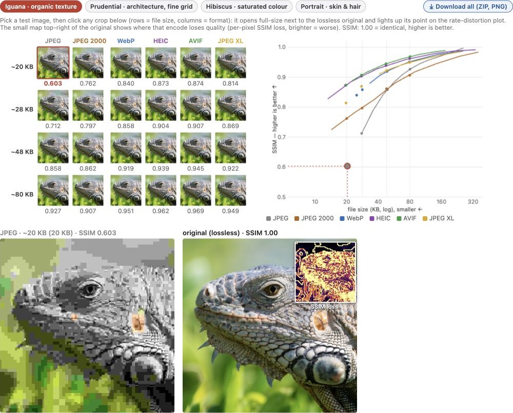
Several formats reuse still-frame tools from video coding; others are designed specifically for images. Their compression is not interchangeable, and equal quality-slider values are not a meaningful comparison.
- HEIF is a container; HEIC commonly denotes HEVC-coded images within it. Bit depth and supported features depend on the codec profile and application.
- WebP provides lossy and lossless coding, alpha, and animation; its lossy and lossless paths use different coding tools.
- AVIF stores AV1-coded still images, with profiles supporting high bit depth and HDR.
- JPEG XL supports lossy and lossless images and reversible recompression of compatible JPEG files. That reversibility is a dedicated mode, not a promise about arbitrary conversions through decoded pixels.
Modern codecs can use spatial prediction, adaptive transforms, and context-dependent entropy coding. JPEG already predicts DC coefficients, so it is inaccurate to say it has no prediction at all. A meaningful comparison fixes image dimensions, color interpretation, and output precision, then measures size, quality, encode/decode cost, and compatibility. Rankings can change with content, metric, and encoder settings.
Learned compression replaces a fixed analysis transform with a network that maps pixels to latent coefficients. Quantize and entropy-code those coefficients, then reconstruct with a synthesis network. Training balances estimated rate and distortion, $\mathcal L=R+\lambda D$. The probability model must match the coded symbols; both sides need compatible model definitions and numerical behavior. A perceptual loss can favor plausible texture over pixel accuracy. JPEG AI has a published core coding standard, ISO/IEC 6048-1:2025; standardization does not imply universal decoder availability.
Intra prediction estimates a block from already reconstructed neighbors and codes the residual. A smooth continuation can then require few residual bits. Adaptive transform sizes change the tradeoff between compactly describing broad structure and following local boundaries. Context-dependent entropy coding assigns code lengths using nearby symbols or other available information. These tools improve the statistical description of the image; perceptual quantization decides which errors to permit. In-loop filtering, where a codec specifies it, also changes the reconstructed reference seen by subsequent predictions, so encoder and decoder must agree on it.
8.11.8 Other formats: TIFF and GIF⧉
TIFF is a flexible container whose compression may be lossless or lossy. It can store integer and floating-point samples and multiple images; application-specific Photoshop layers are not equivalent to universally supported TIFF pages. Test interchange with the destination software.
GIF losslessly compresses indexed pixels, with at most 256 entries in each color table and a transparent index rather than continuous alpha. Converting a photograph to that palette can lose substantial color information before compression. Animation can use different tables in different frames.
For processing, keep the original raw and use an intermediate format with sufficient precision and range. For delivery, choose a supported format, inspect the actual export, and retain its color metadata. When reporting compression results, name the encoder, version, settings, and metric.
Match compression to the task. A visual metric can guide photographic delivery, but masks, measurements, and intermediate images may require exact samples. Lossless refers to the codec input, not to every conversion that preceded it.
Recap: big lessons of this chapter
JPEG combines optional chroma subsampling and coefficient quantization with lossless coding. Perception helps allocate the loss, while signal statistics help encode what remains. Neither the transform nor entropy coding alone produces the large lossy savings.
Match compression to the task. A visual metric can guide photographic delivery, but masks, measurements, and intermediate images may require exact samples. Lossless refers to the codec input, not to every conversion that preceded it.