18.5 Local Laplacian filtering and other multiscale methods⧉
A two-scale method makes one decision: what is base and what is detail. Real scenes have structure at every scale, the window, the frame around it, the texture of the wall, and a single split has to put each of them on one side. Multiscale methods decompose the image into a pyramid of frequency bands (Chapter 6.6, Pyramids and wavelets) and treat each band on its own terms, which is closer to how vision processes contrast (Chapter 18.1, Tone mapping and perception). The difficulty is that the bands are not independent: reducing the coefficients of one band near an edge, without matching changes in the others, distorts the edge, and the naive version of the idea produces halos, broad ramps of brightness toward the other side of each strong edge. This chapter follows the three answers to that problem, from a model of adaptation to the local Laplacian filter.
18.5.1 Multiscale models of adaptation⧉
Pattanaik, Ferwerda, Fairchild and Greenberg built a tone-mapping operator out of a model of vision Pattanaik et al. 1998. They decomposed the scene into band-pass contrast images, applied to each band a gain control that models the eye's adaptation and its sensitivity to contrast at that scale, and then ran the model in reverse for the display, so that the displayed image would produce the same responses in the viewer as the scene did in an observer. The goal was appearance reproduction in the full sense of Part 18, Tone mapping and display, including the loss of acuity and color in dim scenes. The model was expensive and its band-by-band gains produced halos at strong edges, but it set out the idea the later methods kept: range compression is a gain applied to contrast, scale by scale.
18.5.2 Subband companding: Li, Sharan and Adelson⧉
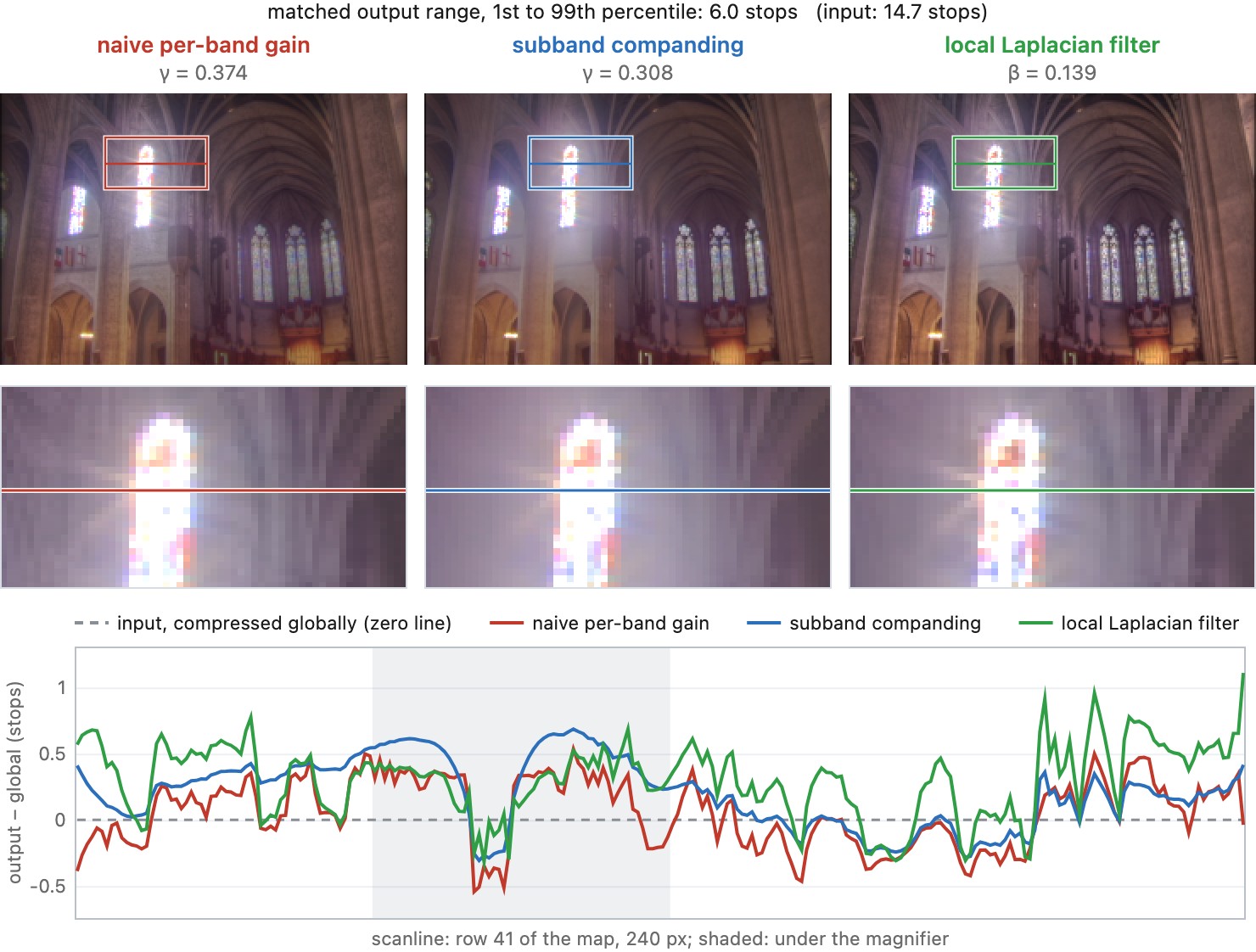
Li, Sharan and Adelson took the signal-processing route and asked why multiband gain control produces artifacts at all Li, Sharan & Adelson 2005. Their operator decomposes log luminance with a filter bank, measures in each band a local activity, the smoothed magnitude of the band's coefficients, and multiplies the band by a gain that falls as activity rises, of the form $(A/\delta)^{\gamma-1}$ with $\gamma<1$, so that strong local contrast, an edge, is compressed while weak contrast, texture, is kept. Their analysis identified two sources of distortion. A gain that varies as fast as the band itself modulates the signal and creates new frequencies; the gain map must vary more slowly than the band it multiplies. And gains computed independently per band disagree at an edge, whose energy spreads across several bands; aggregating the activity across neighboring scales into one map keeps the bands consistent. With an oversampled, symmetric filter bank and smooth aggregated gains, a step edge is bent much less than by independent per-band gains. At strong compression a broad glow can still remain around a very bright region: at a matched compression of six stops on the church interior of Figure 18.5.1, companding leaves the widest glow of the three methods around the window, about two thirds of a stop.
The paper's second contribution is in its title, companding. The same machinery run in reverse expands a compressed image back toward its original range, so an HDR image can be compressed into an ordinary 8-bit picture that looks right on a standard display and still be expanded later, much as an audio compander compresses a signal for transmission and expands it at the other end. It anticipates the backward-compatible encodings of Chapter 17.7, Encoding HDR images.
18.5.3 Local Laplacian filters⧉
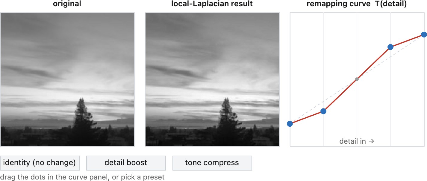
The local Laplacian filter of Paris, Hasinoff and Kautz avoids the problem of consistency between bands by construction Paris et al. 2011. It never multiplies a coefficient by a gain. For each coefficient of the output's Laplacian pyramid, at level $\ell$ and position $p$, it takes the value $g$ of the input's Gaussian pyramid at the same place, remaps the whole input with a pointwise curve $r_g$ centered on $g$, and copies the corresponding coefficient of the remapped image's Laplacian pyramid. The curve treats departures from $g$ smaller than a threshold $\sigma$ as detail and larger ones as edges, with separate slopes for each (Chapter 10.4, Local Laplacian filters).
For tone mapping, the filter runs on log luminance with the edge slope $\beta$ below one, which compresses large departures from the local reference, the steps between a window and a wall, while the detail slope keeps or enhances small ones. Because each coefficient comes from a remapping of the actual image around a reference value, rather than from a gain applied to a band, the result has no halos at the edges a blurred base would cross. Its compression is limited by the same construction: at the usual settings, with the detail exponent at one and the threshold around 1.3 stops, it does not bring the church interior below four or five stops in the comparison figure, and a global curve usually finishes the job. The price was cost: the direct algorithm builds a pyramid per coefficient. Aubry and colleagues showed that remapping around a small set of reference values and interpolating gives the same result to good accuracy, at the cost of a few dozen pyramids, fast enough for interactive editing Aubry et al. 2014, and its implementation is a standard example of a schedule for image-processing pipelines (Part 29, Making computational photography code fast).
18.5.4 Pyramids in exposure fusion and phones⧉
The same pyramid machinery underlies exposure fusion, which blends a bracket with weights that are themselves blended across the levels of a pyramid so that the transitions are invisible (Chapter 18.4, Exposure fusion). The two methods meet in phones. HDR+ merges a burst of short exposures into one image with more range than the display, then renders it by synthesizing a short and a long exposure from the merged image and fusing them with a variant of exposure fusion Hasinoff et al. 2016 (Chapter 17.6, HDR+ and burst imaging on phones). A pyramid blend of synthetic exposures is a multiscale local tone mapper, and an efficient one.
Figure 18.5.1 puts the two gain-control methods of this chapter and the local Laplacian filter side by side on one radiance map, each set to the same overall compression.