45.7 Problem Set 4 — High dynamic range🔗⧉

Problem Set 4: HDR and Tonemapping. Due Wednesday October 14, 9:00pm.

45.7.1 Summary🔗⧉

• merge N bracketed images into an HDR image
• tone mapping with Gaussian and Bilateral blurs

Important.

To merge images to HDR, we will work with images encoded linearly. Most of the digital images you may encounter are encoded with a gamma of $2.2$ (in particular those of the handout). Therefore, in this problem set, you will have to undo the gamma $2.2$ from your inputs before merging them to HDR. You will also have to apply a gamma $2.2$ to the images you output in the linear domain (e.g. after tone-mapping). You can use the gamma_code function from problem set 1 that can be found in basicImageManipulation.cpp to do this. We assume all the inputs and outputs of the functions in this problem set are in the linear space (i.e. you will need to undo the gamma before you call the function and you will need to apply gamma after you tone map).

In the whole assignment, we will only work with images of static subjects and the camera hasn't moved between shots in the same sequence.

45.7.2 HDR merging🔗⧉

Consult the course slides for the overall HDR merging approach. We will first compute weights for each pixel and each channel to eliminate values that are too high or too low. We will then compute the scale factor between the values of two images, to determine their relative exposures.

Finally, we will merge a sequence of images using a weighted combination of the individual images leveraging the weights and scale factors. The slide “Assembling HDR” in lecture 6 might be helpful here.

• 1.a Weights. Write a function Image computeWeight( const Image &im, float epsilonMini=0.002, float epsilonMaxi=0.99) that returns an image with pixel value 1.0 when the corresponding pixel value $v$ of im satisfies epsilonMini $\le v \le$ epsilonMaxi, and 0.0 otherwise. Both bounds are included: use >= and <=, not > and <. This matters for the special cases of question 2, which call it with epsilonMaxi $= 1.0$ to keep pixels that are fully bright (exactly 1.0) and with epsilonMini $= 0.0$ to keep pixels that are fully dark (exactly 0.0). The weights are computed on a per pixel and per channel basis.
• 1.b Factor. Now that we know which pixels are usable, we can compute the multiplication factor between a pair of images. Write a function float computeFactor(const Image &im1, const Image &w1, const Image &im2, const Image &w2) that takes two images and their weights computed using the above method, and returns a single scalar corresponding to the median value over all pixels and channels of im2/im1 for pixels that are usable in both im1 and im2. Add an epsilon of $10^{-10}$ to the pixels of im1 to avoid divide by 0 errors.

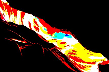
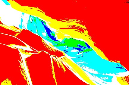
Figure 1. The weights computed from the ante2 image sequence using the default parameters provided in computeWeight. You can see this output after running testComputeFactor.

With these two methods, we know which pixels are usable in each image and what the relative exposures between the images is. With this information we are ready to merge a sequence of images to a single HDR image.

For the rest of the problem, you can assume that the first image in the sequence is the darkest, and that images are given in order of increasing exposure.

For each image in the given sequence, you need to compute its multiplicative scale factor ($k_i$ in the equation on the “Assembling HDR” slide from lecture 6). This requires computing the scale factor between adjacent images in the sequence using computeFactor, then chaining them together. For example, if you have the factor between image 3 and image 2 and image 2 and image 1, you can compute the factor between image 3 and image 1 by chaining the factors together:

You should should pick one of the images as the reference' image (e.g. the darkest image), and compute the factors with respect to it. This means that each image's $k_i$ value will be relative to your reference' image i.e. you will compute it only up to a global scale factor.

Pixels badly exposed in every image.

See slide “Special Cases” in lecture 6. A pixel that is too bright even in the darkest image is clipped in all of them. The darkest image's value, possibly exactly 1.0, is then the best you have: it is a lower bound on the true value, but no exposure does better. Likewise, a pixel that is too dark even in the brightest image is best measured by the brightest image, even at exactly 0.0. So compute each image's weights with computeWeight and these ranges, both ends included, with the images ordered from darkest to brightest:

With two images there is no middle one: the first takes the first row and the second the last. The weights are per channel, so one pixel's red may come from a different exposure than its green, for example when red is clipped in one image and green is not. That is intended.

Use these same weights when you call computeFactor on each pair of adjacent images. The extra pixels they keep never count in a pair: a pixel at 1.0 in the darker image of a pair is also above epsilonMaxi in the brighter one, and a pixel at 0.0 in the brighter image is also below epsilonMini in the darker one, so the median is unchanged.

If a pixel still has weight 0 in every image, use the first image's value, so that you never divide by 0. With the ranges above this only happens when two consecutive exposures are more than epsilonMaxi/epsilonMini, about 500 times, apart.

As you merge pixels, do not forget to scale them with the factors computed above: computeFactor returns the median of im2/im1, so each image's values are brought to the reference exposure by dividing them by that image's $k_i$ relative to the reference (with the darkest image as reference, $k_1 = 1$ and the brighter images have $k_i > 1$).

To test your method, you can write out the output image scaled by different scaling values. testMakeHDR in a4_main.cpp illustrates the process for the design image sequence.

• 2.a Merge to HDR Write a function Image makeHDR(vector<Image> &imSeq, float epsilonMini=0.002, float epsilonMaxi=0.99) that takes a sequence of images as input and returns a single HDR image.
• 2.b Create three small exposure sequences of your own to use for testing and debugging makeHDR, and include them in your submission (see the naming scheme below). They should be images you construct, not photographs: decide what the scene is, then make each exposure from it, so that you know what the merged result should be. For each sequence, say what the scene is, why you chose it, how you made the exposures, and what you expect makeHDR to return. (Answer in the form)

Your test images.

Put the images you make in Input/debug/, lowercase, at most $256\times256$ pixels. An exposure sequence is named hdr_<n>_<i>_<what>.png, with <n> from 1 to 3 for the sequence and <i> from 1 for its darkest exposure, in order of increasing exposure, like the provided sequences. Later in the set you also make tone_1_… png to tone_3_… png. make prepare copies Input/debug/ into your submission, so they travel with your code. Keep the code that makes them, and the code that runs your functions on them, in a4_main.cpp, and write the results into Output/ under the same name with _out added.

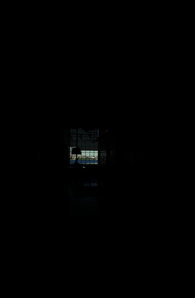
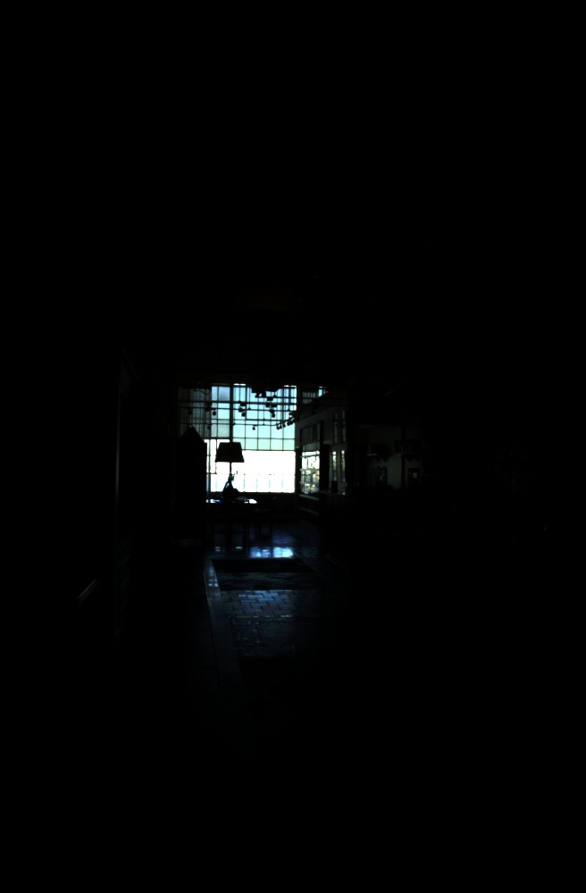
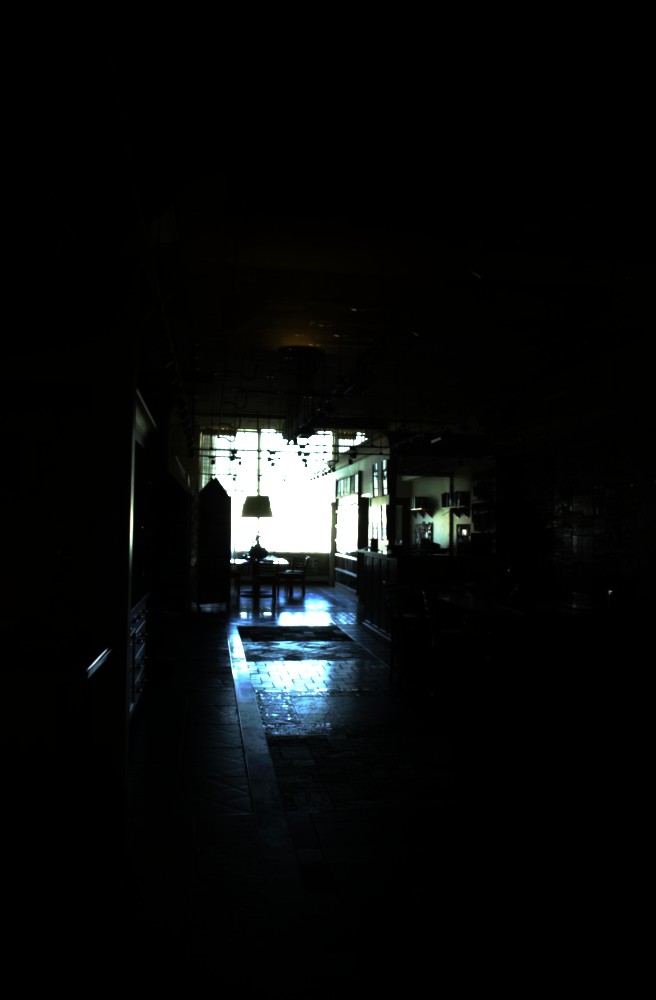
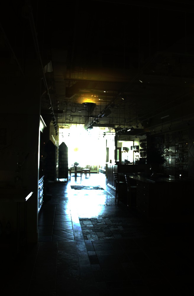
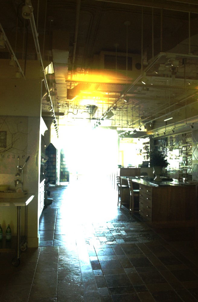
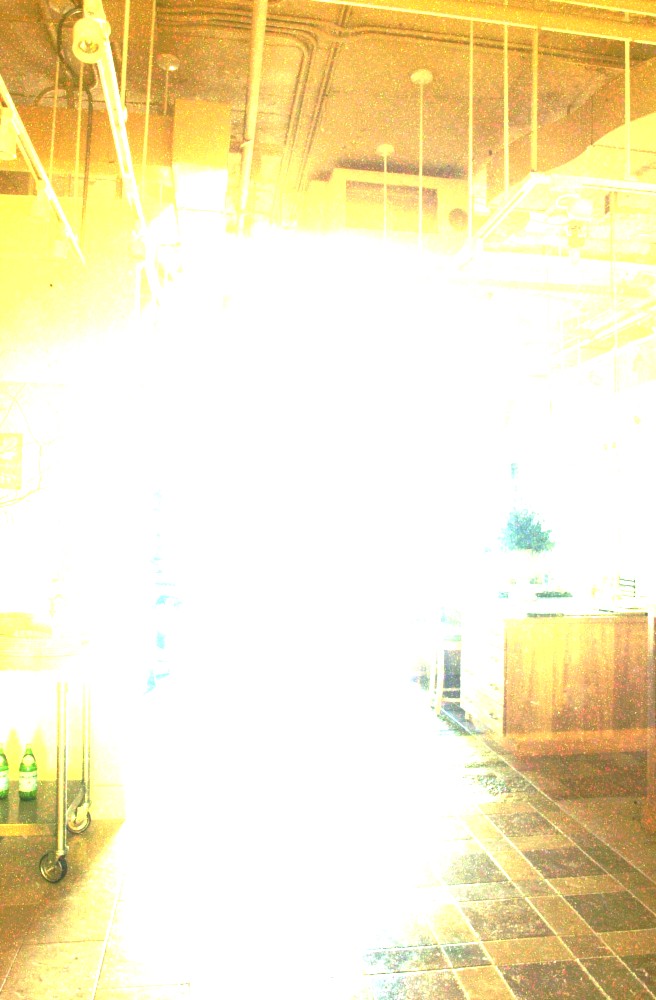
Figure 2. The HDR image created from the design image sequence clipped to different ranges. You can see this output after running testMakeHDR.

45.7.3 Tone mapping🔗⧉

We have assembled our first HDR image, but this image still cannot be displayed properly on our low dynamic range screen. Let's implement tone mapping to remap the HDR information to a displayable range. Make sure you understand the slides “Contrast reduction in log domain” in order to combine the base luminance, detail and brightness scaling factor.

Your tone mapper will follow the method studied in class. The function is called toneMap, declared in hdr.h as Image toneMap(const Image &im, float targetBase=100, float detailAmp=3, bool useBila=false, float sigmaRange=0.1). It takes as input an HDR image, a target contrast for the base (lowpass) layer, an amplification factor for the detail, a Boolean to switch the lowpass/highpass separation between the bilateral filter or Gaussian blur, and the bilateral filter's range standard deviation, used when useBila is true.

As described in the lecture, our goal is to reduce the contrast from the HDR image (say, 1:10000) to what the display can show (say 1:100). Although gamma correction might seem like the first thing to consider, this results in washed out images, as shown on the gamma compression slide in lecture 7. The colors are actually okay (they're all there) but the high frequencies are washed out. We therefore want to work on the luminance, and increase the high frequencies. We also want to work in the log-domain since the human eye is sensitive to multiplicative contrast (recall lecture 1).

We want to modify only on the log-luminance:

• 3.a In the function toneMap, first decompose your image into luminance and chrominance using the function from problem set 1 std::vector<Image> lumiChromi(const Image &im) that can be found in basicImageManipulation.cpp. We also provide you the reciprocal function lumiChromi2rgb. lumiChromi divides by the luminance. It is never zero on the provided sequences; if you try your own images, guard that division.
• 3.b Next, compute a log10 version of the luminance. To avoid taking the log of 0, first replace every value below the image's smallest non-zero value (in practice, the zeros) by that smallest non-zero value; leave the other pixels as they are.

We recommend you do this by first implementing the helper function float image_minnonzero(const Image &im), followed by Image log10Image(const Image &im), for which we have written function signatures and comments for you. Then, call log10Image with the luminance image as the argument.

Next, we want to extract the detail of the (log) luminance channel. We do this by blurring the log luminance, and subtracting this from the original log luminance. If you recall problem set 2, this gives you the details (high frequencies).

• 3.c You are ready to compute the base (blurry) luminance. We will implement two versions: Gaussian blur and bilateral filtering, which will be chosen based on the value of the input parameter useBila. In both cases, we will use a standard deviation for the spatial Gaussian equal to the biggest dimension of the image divided by 50. The parameter truncateDomain should be set to the default value of 3.

You are welcome to use your own implementation of filtering methods, but you can also use our versions in filtering.cpp.

• 3.d Given the base, compute the detail by taking the difference from the original log luminance.
• 3.e What differences do you expect to see in your tone mapping results when the base comes from a bilateral filter rather than a Gaussian blur, and why? Answer about the tone-mapped images, not the two filters alone: where in a picture do you expect the two results to differ? (Answer in the form; hint: the slides might help.)

At this point we have a detail image and a base image. Our goal is to reduce the contrast on the base image while also preserving (or even amplifying) the details. The slides “Contrast Reduction in log domain” might be helpful here.

• 3.f Compute the scale factor k in the log domain that brings the dynamic range of the base layer to the given target (that is, the range in the log domain should be log10(targetBase) after applying k). Scale the base image by the factor k to reduce the contrast, and multiply the details (in the log domain) by detailAmp. Next, add the scaled base and amplified detail to obtain your new log luminance.

Make sure to add an offset that ensures that the largest base value will be mapped to 1 once the image is put back into the linear domain

We have provided two new functions for you that you might find useful: float Image::min() const and float Image::max() const to get the minimum (respectively maximum) value of an image.

• 3.g Convert this new luminance back to the linear domain (you may want to separately implement Image exp10Image(const Image &im)). Then, reintegrate the chrominance into the resulting image. We've provided the function Image lumiChromi2rgb(const vector<Image> & lumiChromi) in basicImageManipulation.cpp which might be helpful.
• 3.h Create three small HDR images of your own to use for testing and debugging toneMap, and include them in your submission, named tone_1_… png to tone_3_… png under Input/debug/ as above. They should be images you construct, not photographs. A PNG only holds values up to 1, so make each one in code, save it divided by its maximum, and keep the code that makes it. For each one, say what the image is, why you chose it, what parameters you run toneMap with, and what you expect the output to look like. (Answer in the form)

Enjoy your results and compare the bilateral version with the Gaussian one. Use the functions testToneMapping_ante2, testToneMapping_ante3, testToneMapping_design, testToneMapping_boston in a4_main.cpp to help test your tone mapping function. Feel free to try them on your own images!

Note: The bilateral filter on the design image sequence takes a very long time. It is not necessary to test bilateral filter tone mapping for this image sequence. If you do test it, you likely won't get exactly the same image as given in the slides because it was generated with different parameters.

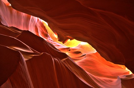
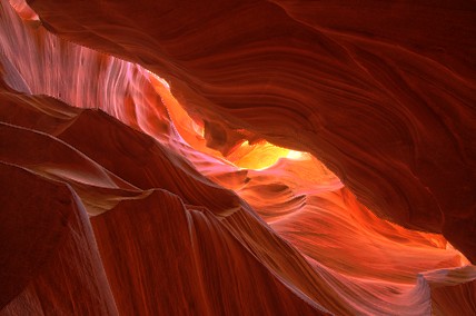
Figure 3. Tone mapping of the ante2 image sequence using the parameters provided in testToneMapping_ante2

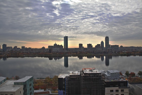
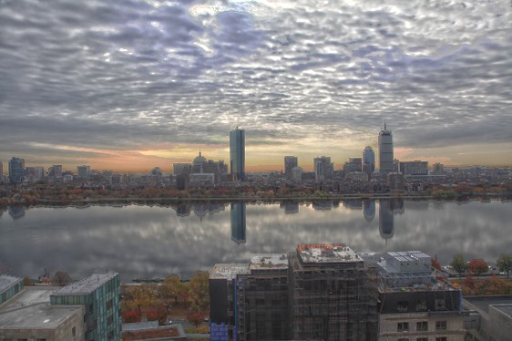
Figure 4. Tone mapping of the boston image sequence using the parameters provided in testToneMapping_boston

45.7.4 Extra credit (10% max)🔗⧉

• (5%) Deal with image alignment (e.g. the sea images). We recommend Ward's median method <http://www.anyhere.com/gward/papers/jgtpap2.pdf> but probably single-scale to make life easier yet slower. Alternatively, you can simulate the clipping in the darker of two images.
• (5%) Derive better weights by taking noise into account. You can focus on photon noise alone. This should give you an estimate of standard deviation (or something proportional to the standard deviation) for each pixel value in each image. Use a formula for the optimal combination as a function of variance to derive your weights. This should replace the thresholding for dark pixels, but you still need to set the weight to zero for pixels dangerously close to 1.0.
• (5%) Write a function to calibrate the response curve of a camera. See <http://www.pauldebevec.com/Research/HDR/>
• (10%) Implement the bilateral grid for fast bilateral filtering. See <http://groups.csail.mit.edu/graphics/bilagrid/> with more mathematical justifications at <http://people.csail.mit.edu/sparis/publi/2009/ijcv/Paris_09_Fast_Approximation.pdf>
• (10%) Hard: deal with moving objects

45.7.5 Submission🔗⧉

Turn in your files to the online submission system and make sure all your files are in the asst directory under the root of the zip file. If your code compiles on the submission system, it is organized correctly. The submission system will run code in your main function, but we will not use this code for grading. The submission system should also show you the image your code writes to the ./Output directory

In the submission system, there will be a form in which you should answer the following questions:

• How long did the assignment take? (in minutes)
• Potential issues with your solution and explanation of partial completion (for partial credit)
• Any extra credit you may have implemented and their function signatures if applicable
• Collaboration acknowledgment (you must write your own code)
• What was most unclear/difficult?
• What was most exciting?