30.3 Video editing⧉
Video editing puts alignment, flow, warping, and robust per-pixel statistics to use in selecting and assembling footage. The pattern is the same as in the rest of the part: almost every "video effect" is align the frames, then reduce or select across time, or re-time the timeline.
A recurring principle is: establish a correspondence, then transport pixels along it. The reduce-over-time filters in this chapter are the main exception. They produce striking results, a long exposure made from a clip, a crowded plaza emptied of people, with no correspondence estimated at all. Once the frames are registered, each pixel's time series is processed independently, exactly the Eulerian move that Chapter 38.3, Motion and video magnification made. This coda closes the loop: the part opened by insisting on correspondence, and ends by showing how much you can do by refusing it.
30.3.1 Non-linear editing: the timeline metaphor⧉
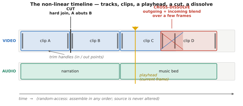
Start with the substrate. Traditional linear tape editing assembled source segments onto an output tape in sequence. Changing a segment’s duration could require rebuilding later material, although insert editing permitted some local replacements. Physical film splicing is a different editing process. Digital non-linear editing (NLE) broke that constraint. Clips are stored as random-access files, so you assemble them on a timeline in any order, re-arrange them freely, and the edit itself is nothing more than a list of references with in- and out-points into the source media. The edit is non-destructive. The original footage is never altered, exactly the non-destructive-editing discipline already established for stills in Chapter 8.12, Recap ISP, non-destructive editing. "Non-linear" names this decoupling: the order in which you edit no longer has to match the order of playback.
The timeline itself is a small visual language (Figure 30.3.1). Parallel video and audio tracks run left to right; clips sit on them with draggable trim handles; a playhead marks the current time. Edits come in two flavors. A cut is a hard join: one clip ends, the next begins, on the same frame. A transition is a soft join: a cross-dissolve, wipe, or fade that blends the outgoing and incoming clips over a short overlap. A cross-dissolve is literally the temporal cross-fade of Chapter 11.3, Morphing and Chapter 30.4, Frame interpolation and slow-motion synthesis: $(1-t)$ of the old clip plus $t$ of the new, swept over the transition. This is why it ghosts in exactly the same way when the two shots are misaligned, A flow-aware morph can help for compatible shots, but can badly distort unrelated scenes; a dissolve may be the intended visual transition.
The timeline matters here because it is the substrate the rest of the chapter manipulates. Summarization shortens it; the reduce-over-time filters collapse a stretch of it to a single frame; transcript editing re-orders it from text; and slow motion and speed ramps (the subject of Chapter 30.4, Frame interpolation and slow-motion synthesis) re-time it. Everything below is an operation on this one object.
The craft of editing (pacing, continuity, the cut on action, the rhythm that makes an edit invisible) is a whole art, and we touch only its computational hooks; the human side is out of scope here.
30.3.2 Summarization: keyframes, fast-forward, and highlights⧉
The goal of summarization is to compress watching time, not file size, turning an hour of footage into something glanceable or skimmable. Three primitives recur, each optimizing something different.
Representative frames (keyframes). Pick a small set of frames that cover the content. The simplest cover is one frame per shot: detect shot boundaries where the inter-frame difference spikes (a cut), and take a representative from each segment. A slightly richer version clusters the frames by appearance and keeps a medoid per cluster. The output is a contact sheet or storyboard, a static glance at a dynamic thing.
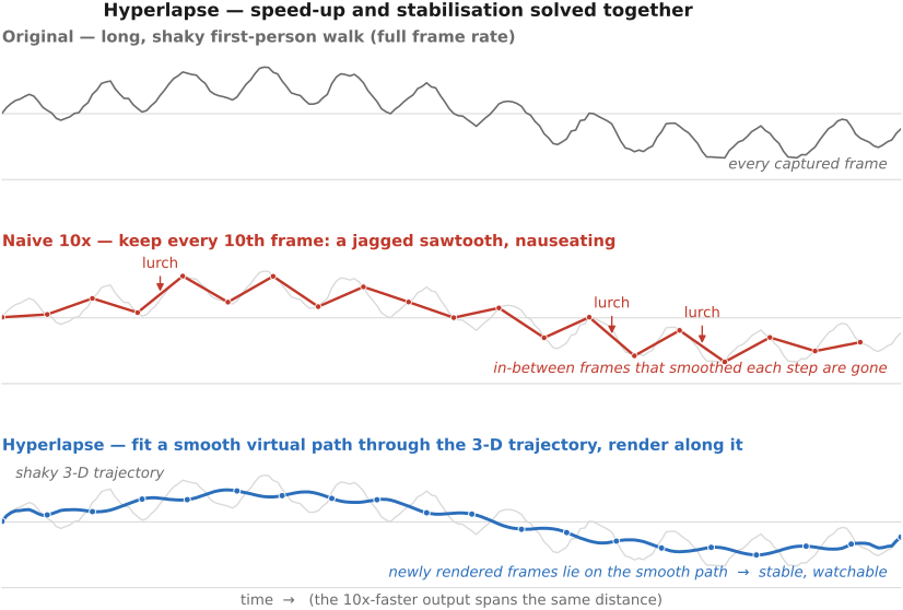
Adaptive fast-forward and hyperlapse. The problem is speeding up long first-person footage, a head-mounted camera on a hike, say. The naive fix, dropping nine of every ten frames for a $10\times$ speed-up, is unwatchably shaky: every footfall that was a small jolt at normal speed becomes a violent lurch when the in-between frames that smoothed it are gone. Hyperlapse Kopf et al. 2014 solves this by treating speed-up and stabilization as one problem. It reconstructs the camera's path in 3-D from the footage, chooses a smooth virtual path through that trajectory, and renders new frames along the smooth path rather than sampling the jittery original ones. The path-smoothing is exactly the camera-trajectory smoothing of Chapter 30.6, Video stabilization and rolling-shutter correction, and the rendering leans on the motion estimate of Chapter 12.8, Optical flow: hyperlapse is stabilization fused with time compression. The speed can also be content-adaptive: slow down over eventful, interesting stretches and race through dull ones, so the summary spends its frames where they matter (Figure 30.3.2).
Highlight and event detection. Rather than cover the whole video, surface only the interesting parts. Score frames or short segments by some notion of interestingness, saliency, motion energy, faces, audio peaks, or a learned interestingness model (forward-ref Chapter 7.2, Machine learning), then keep the top-scoring segments. This is the engine behind automatic sports highlights and action-camera "best moments." What counts as a highlight is largely a learned, task-specific judgement.
30.3.3 Fun temporal filters: reduce-over-time⧉
Now consider simple temporal filters. Once the frames of a clip are aligned (stabilized, so the static scene sits still from frame to frame), apply a single per-pixel reduction across time:
Read back: at each pixel location $\mathbf p$, collapse its whole time series $\{I_t(\mathbf p)\}$ to one value with some reducer. The reducer is the entire effect, and four choices give four classic looks (Figure 30.3.3).
Mean over time is an approximation to a long exposure from video: $O = \tfrac1N\sum_t I_t$. Moving water silks into a smooth sheet, headlights stretch into continuous light ribbons, a passing crowd blurs into translucent smears. Average in linear light for a radiometric integration. Gaps between frame exposures can leave broken trails, and rolling shutter or nonlinear processing changes the result. Independent equal-variance noise falls by $1/\sqrt N$, as in Multiple exposure imaging, but reframed as an effect rather than a fix. Same align-then-average pattern, opposite intent.
Median over time is robust background recovery, the people-remover: $O(\mathbf p) = \operatorname{median}_t I_t(\mathbf p)$. Anything transient, a tourist crossing the frame, a passing car, occupies any given pixel only briefly, so across the stack it is an outlier, and the median rejects outliers by construction. The background is recovered reliably only where it is visible in a majority of valid samples and remains stable in appearance. A stationary person or a persistently crowded pixel defeats this simple rule. This is the same robustness that made the median the denoiser of choice for salt-and-pepper noise back in Part 13, Denoising; here it rejects temporal outliers instead of spatial ones.
Max over time is bright-streak accumulation: $O(\mathbf p) = \max_t I_t(\mathbf p)$, keep each pixel’s maximum. Define whether the maximum is channelwise, which can synthesize colors from different frames, or selects the RGB triplet with maximum luminance. Stars smear into star trails as the sky rotates; light-painting, lightning, firework tails, a night runner's headlamp all leave their brightest trace. Min over time is the dual: the darkest value each pixel saw, handy for dropping specular flashes or recovering a persistently dark background.
There is a fifth move that is not a reduce but a pick. Instead of collapsing each pixel's time series with a statistic, choose the best frame per region:
where $s(I_t,\mathbf p)$ scores how good frame $t$ is at location $\mathbf p$. This is the "everyone smiling / no blinks" group-portrait trick: shoot a short burst, and for each face splice in the one frame where that person's eyes are open and they are smiling, then merge the pieces seamlessly. It is interactive digital photomontage Agarwala et al. 2004 (select-the-best-pixel over a stack) applied to a brief burst. The seamless merge is precisely the cut-then-reconstruct pipeline of Part 10, Edges matter: a graph-cut seam decides where to switch between source frames (Chapter 10.9, Seam optimization) and a gradient-domain blend hides the residual mismatch (Chapter 10.8, Poisson image editing, Chapter 20.3, Blending). The scoring function $s$, "eyes open, smiling", is a learned face attribute (forward-ref Chapter 7.2, Machine learning) (Figure 30.3.4).
One prerequisite governs all of these: the frames must be registered. On a tripod they already are; on handheld video they are not, and you must stabilize or align first (Chapter 30.6, Video stabilization and rolling-shutter correction), or the static scene smears along with the moving parts and the effect collapses. This is the same align-then-combine discipline that high-dynamic-range (HDR) and panorama capture demanded: register first, reduce second.
This is another Eulerian use of temporal data. Every other application in this part estimated a correspondence and transported pixels along it. These filters do not: after a global registration, each pixel is treated in isolation, its time series reduced with no notion of where anything moved to. That is the Eulerian stance of Chapter 38.3, Motion and video magnification: process the signal at a fixed pixel rather than follow matter through space, and it is exactly why these effects are so cheap and so robust. This is the exception.
30.3.4 Transcript-based editing⧉
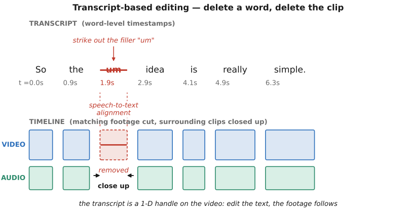
Transcript-based editing lets you edit a talking-head video through its transcript.
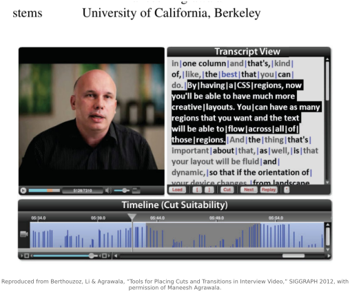
The pipeline is short. Run speech-to-text (automatic speech recognition, or ASR) with word-level timestamps (forward-ref Chapter 7.2, Machine learning; here ASR is a black box). Now every word in the text is pinned to a moment in the audio, and the audio is locked to the video. So a chain of alignments connects text to picture: delete a sentence in the transcript, and the matching clip is removed from the timeline; reorder paragraphs, and the shots reorder to follow. The transcript becomes a one-dimensional handle on a two-dimensional medium. Text is enormously easier to scan and rearrange than a wall of thumbnails (Figure 30.3.7).
A practical use is filler-word removal. Find every "um," "uh," "you know," and "like," strike them in the text, and the corresponding micro-segments vanish from the timeline, tightening the cut automatically, a useful candidate edit that still needs checking: these words can carry meaning, and timestamp errors or abrupt audio boundaries can spoil a cut. The same handle gives search-and-replace navigation ("jump to where they said aperture") and, with a voice model, overdub: retype a misspoken word and have it re-synthesized.
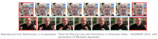
The research root is Berthouzoz, Li and Agrawala Berthouzoz et al. 2012, Tools for Placing Cuts and Transitions in Interview Video, which automated finding clean, well-hidden cut points (at sentence and pause boundaries) in interview footage. That work is the academic ancestor of the Descript-style transcript editors now in wide use.
It works because speech is a clean alignment signal for dialogue-driven video; word timestamps provide a convenient index into the timeline, subject to recognition and alignment errors. The limits follow from that same dependence. It is for spoken-word content; for action, music, or wordless footage there is no transcript to grab. And a jump cut between two non-adjacent kept segments can look abrupt because the speaker's head jumps position, so the seam may need a transition or a flow-based seam-hiding frame interpolation (Chapter 30.4, Frame interpolation and slow-motion synthesis) to smooth it over, which is one more use of the part's interpolation machinery.
30.3.5 In-betweening: synthesizing the frames an edit needs⧉
Editing sometimes synthesizes footage. In-betweening is the photographic version of the animator's craft: given two frames $I_0$ and $I_1$, two adjacent frames of a clip, or two shots you want to bridge, produce the frame $I_t$ that belongs between them at time $t\in(0,1)$. It is the engine of the editor's most common temporal effects: retiming a clip to a different speed, up-converting a 24 fps source to a 60 fps timeline, smoothing a morph cut between two interview takes so the join is invisible, and faking slow motion from ordinary footage by sampling $t$ on a fine grid. It is exactly a morph carried into time (the correspondence-then-transport principle): you cannot average the two frames in place, because anything that moved leaves a doubled ghost, so you must estimate a correspondence (optical flow, or a learned matcher), warp both frames toward the in-between time, and only then blend.
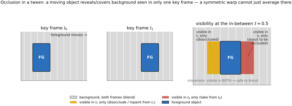
A central difficulty, also present in still-image morphing, is occlusion. A foreground object covers background as it advances and uncovers it as it retreats, so at the in-between time some pixels are visible in only one of the two frames; the blend must reason about visibility: copy a disoccluded strip from the frame that can see it, blend only where both frames agree, and in-paint where neither can (Figure 30.3.8). That visibility logic, plus robustness to large motion, is what separates a true tween from a ghosting cross-dissolve, and it is what pushed the field from classical flow to learned synthesis. We keep this brief because the full development (the flow-warp-and-blend mechanics, Super SloMo's learned intermediate flow, and FILM's large-motion network) is the subject of Chapter 30.4, Frame interpolation and slow-motion synthesis; here we only place in-betweening where the editor reaches for it.
30.3.6 Coda: storyboards, interviews, and where this part lands⧉
Run the timeline forward and you get storyboarding and pre-visualization, planning shots before they are captured; run it in reverse over an existing edit and auto-storyboarding pulls keyframes (the summarization primitive above) to recap what was shot. And the transcript handle plus a multi-track timeline are tailor-made for interview and multi-cam assembly: synchronize several cameras by their common audio, then cut between angles by editing the shared transcript.
We began with motion as physics to model: optical flow, warping, magnification, compression. We turned it into correction (stabilization and rolling-shutter rectification) and then into synthesis: frame interpolation and slow motion that was never shot. We end here with editing: motion as raw material for storytelling. And underneath every effect in this chapter sat one of just two moves: register the frames, then reduce or select across time, or re-time the timeline, the same pattern used elsewhere in the book: align first, then combine or re-time.