4.1 Linear color reproduction and CIE XYZ⧉
A color match reproduces an observer’s responses to light without reproducing its spectrum. For a fixed standard observer, tristimulus coordinates describe these matches with three numbers. The central calculation is linear, but its physical constraints matter: a display can add light from its primaries, not subtract it.
4.1.1 The color reproduction perspective⧉
In principle, measuring color and reproducing it are separate problems. Given light, measurement reports coordinates for its color. Given those coordinates, reproduction builds light on a screen or a page that matches it. You could imagine a camera reporting device-independent measurements to a separate display module, with neither module needing to know how the other works. Much of the notation we actually use comes from treating them together as a reproduction pipeline.
The reason is historical and experimental. Color matching provided a way to measure perceptual color before cone sensitivities could be measured directly. An observer adjusted three fixed primary lights until their mixture matched a test light. The three knob settings were the measurement. These coordinates therefore described amounts of particular reproduction primaries, rather than direct cone responses. Changing the primary lights changed the coordinates of the very same test light. The experiment made measurement possible, but also made the reproduction apparatus part of the measurement convention. Television reinforced the practical importance of a primary-based description: a central engineering task was to get the right picture out of a particular screen.
Metamerism makes this useful. Different spectra can match for the specified observer and conditions. They may cease to match for another observer, or after a change of illumination when the spectra come from reflecting objects. Colorimetry describes the match; it does not by itself predict appearance across different surrounds and adaptation states.
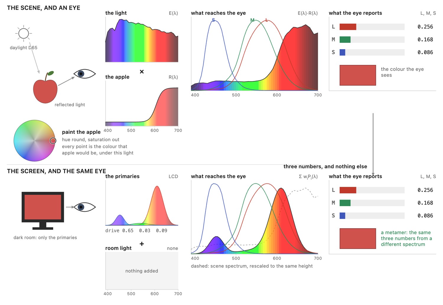
XYZ provides a common reference for device characterization and color conversion. The agreement matters as much as the matrix algebra. With a shared reference, a new display can describe its primaries once instead of requiring a separately standardized conversion from every existing camera or working space. Conversion between two linear tristimulus coordinate systems for the same observer is a matrix multiplication. The shared reference lets those conversions be composed. A camera’s three raw channels generally do not span exactly the standard observer’s matching functions, so its color-correction matrix is an approximation fitted to a calibration set. Nonlinear encodings must be decoded before applying linear-light color matrices.
Changing illumination is another limitation. The illumination multiplies reflectance wavelength by wavelength, whereas a three-channel measurement has already discarded most of that spectral information. A three-by-three chromatic-adaptation transform is a useful model of corresponding colors, not a general solution to spectral relighting. Smooth illumination alone does not make it exact.
A typical rendered-image path includes black-level correction, white-balance gains, demosaicking, camera color correction, tone and color rendering, and output encoding. Implementations combine or reorder some stages. XYZ often enters through the calibration that defines the matrices rather than as a separately stored image. To convert between two linear RGB systems, we can compose an RGB-to-XYZ matrix with an XYZ-to-RGB matrix and apply the resulting matrix directly. The intermediate XYZ coordinates define the conversion without needing to be written into an image buffer. This is why XYZ can be central to a system whose working images are all called RGB.
4.1.2 Analysis vs synthesis and non-orthogonality⧉
First imagine three nonoverlapping, flat sensitivity bands. Measuring the power in each band and emitting the same power within that band would reproduce the three measurements. Human cone sensitivities overlap instead: a light chosen to stimulate one cone type also stimulates others. If we use the sensitivity curves themselves as emission spectra, then scale them by the measured responses, measuring the result applies that overlap a second time. The responses generally change, as Figure 4.1.3 shows. We need to account for how every chosen primary stimulates every analysis channel.
The failing construction is short enough to write out. Emit the sensitivity curves weighted by the responses, $\hat{\mathbf e}=C^{\mathsf T}\mathbf r$, and measure the result: the responses come back as $C\hat{\mathbf e}=CC^{\mathsf T}\mathbf r$. The three-by-three matrix $G=CC^{\mathsf T}$ holds the overlap of every pair of curves, and it is the identity only if the curves are orthonormal. For cones it is far from that, above all for L and M, which overlap heavily, so a light that should excite mostly L comes back measured as a large L and M mixture, and a monochromatic test light is rebuilt as a broad, desaturated one (Figure 4.1.3). The correct weights are $G^{-1}\mathbf r$, which is what the dual basis computes, and they include negative entries: to reproduce the test light with these curves as emitters we would have to subtract light, which is the same wall that real primaries hit in the next section.
Sample an incoming spectrum into a vector $\mathbf e$. Let $C$ be a three-by-$N$ analysis matrix, including wavelength-bin weights, and let the columns of $P$ be three sampled display-primary spectra. Measurement and reproduction are
Thus matching the target requires solving $A\mathbf p=\mathbf r$, where $A=CP$. Each column of $A$ gives the three measured responses to one display primary. If $A$ is invertible, there is a unique algebraic solution. The display can realize it only if every primary weight lies within its allowed range.
Sensitivity curves measure a spectrum; emission primaries construct one. Reusing the sensitivity curves as primaries and the measured responses as weights generally gives the wrong color. Calibrate how each primary stimulates the observer, then solve for its weight.
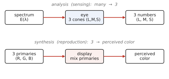
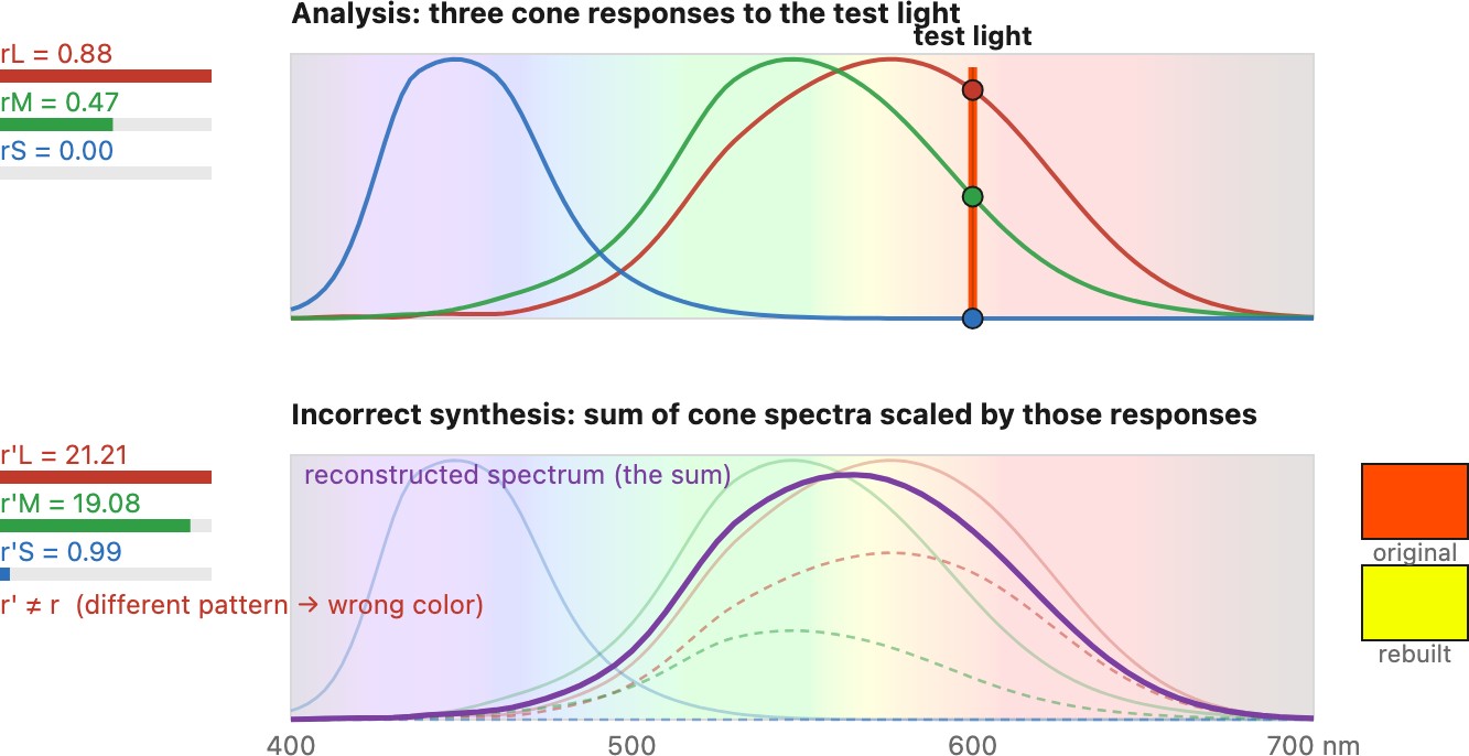
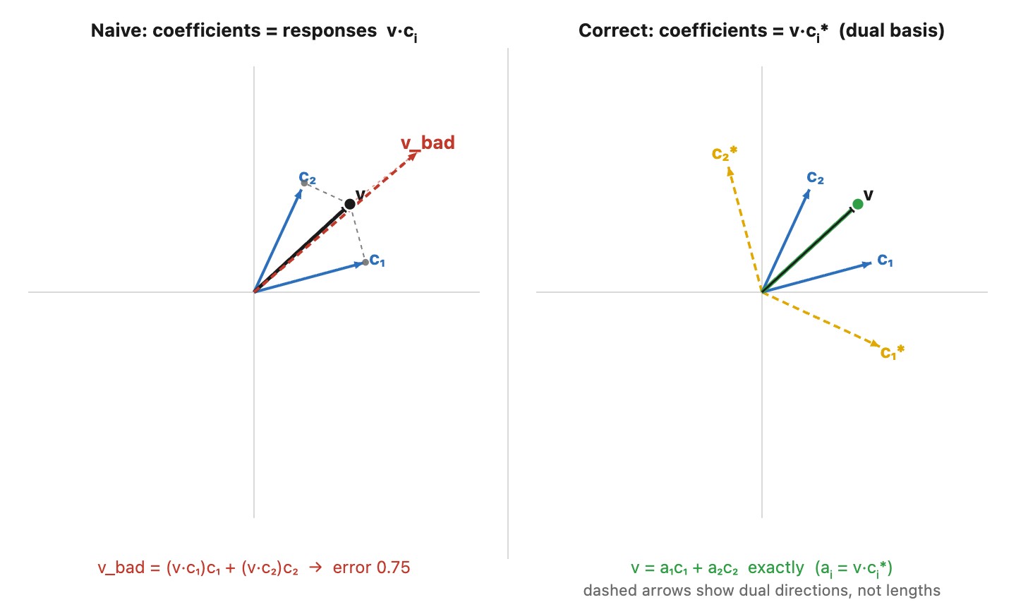
The problem color reproduction actually solves is not quite the textbook one. In linear algebra, reconstruction means rebuilding a vector exactly as a linear combination of basis vectors, so that the result equals the original. Color reproduction asks for less. We do not need the reproduced spectrum to equal the original spectrum, only to produce the same three cone responses, that is, to be a metamer of it. That is a weaker requirement, a match of projections rather than of whole vectors, and it buys a great deal of freedom: the reproduction primaries can be chosen independently of the analysis (cone) vectors, they can be picked to be physically realizable lights, and an in-gamut color can still be matched. Solving the primary-response system gives the coefficients for a given set of primaries; metamerism is what lets us choose those primaries in the first place.
This is where the usual non-orthogonal-basis intuition helps, provided we apply it to the right space. The three primary-response columns need not point along independent cone axes. Solving their linear system compensates for the cross-talk. Merely using a measured cone response as the weight of a similarly shaped emitter applies the cross-talk again. The distinction between taking dot products and solving for synthesis coefficients is familiar from dual bases in linear algebra; here the goal is equality of three measurements, with no requirement to reconstruct the original spectrum.
The algebraic solution can include a negative primary weight. That is a useful coordinate, but a display cannot emit negative light to subtract the unwanted response of another primary. Its physically available mixtures form a restricted set. Metamerism gives us freedom to use a different spectrum for a match; it does not ensure that a particular display's positive mixtures contain a match for every visible color.
The representation labels are a practical type system. A matrix accepting linear RGB cannot be applied directly to encoded RGB merely because both have three components. A luminance and a luma can both be called brightness in conversation while requiring different computations. Before composing two matrices, check that the first one's output has the second one's expected primaries, reference white, normalization, and encoding. The matrix dimensions alone cannot catch these mistakes. This is why color code needs more bookkeeping than an arbitrary three-vector calculation.
Label the representation at each transition. In this part, bare RGB denotes linear values, primes denote a specified nonlinear encoding, and a superscript $\ell$ denotes a specified log encoding. The curve must still be named: a prime does not distinguish sRGB, Rec. 709, or PQ. PQ can encode RGB as well as coordinates used inside ICtCp. A matrix signature states its input and output, for example $M:\mathrm{RGB}_{709}\to\mathrm{XYZ}$. Equal input and output types do not imply an identity operation; exposure scaling is an obvious counterexample.
4.1.3 Color matching and the most standard color space: CIE XYZ⧉
Why measure color through matching experiments rather than directly through cone responses? When the CIE established its 1931 standard, direct measurements of human cone spectral sensitivities were not available. Observers could nevertheless tell when two lights matched. That gave colorimetry an experimental route: define the analysis of a light by measuring its synthesis from adjustable primaries. Metamerism makes this possible because the spectra need not be identical, and the additivity of matches lets the measured coordinates be used for mixtures.
The design of that experiment is why it worked. Psychophysics, putting a number on a private sensation, is slippery: observers disagree, adapt, tire, and shift their answers with the surround and the wording of the task. A matching experiment asks for none of that. It is a null measurement: the observer reports only when the two halves of a field look the same, which people do far more reliably than they rate how different two colors are. Metamerism keeps the answer to three numbers rather than a spectrum, and linearity lets a limited set of measured matches extend to every mixture. The 1931 standard rests on the matching data of Wright and of Guild, about seventeen observers across the two studies, and it still predicts matches for typical observers well enough to anchor color measurement nearly a century later, within the limits of an average observer that the rest of this chapter keeps in view.
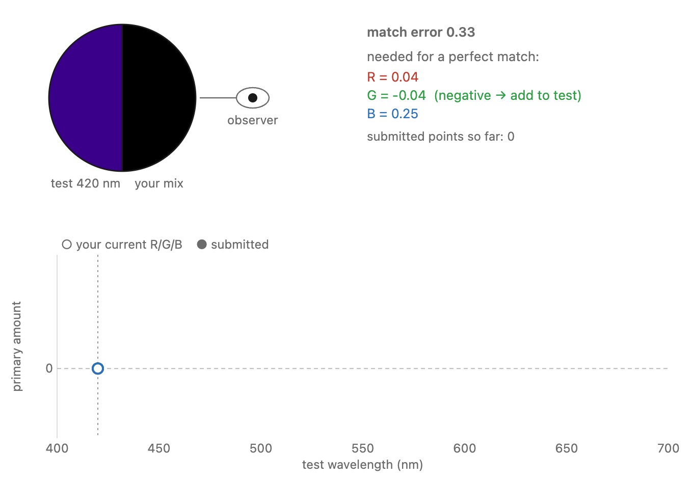
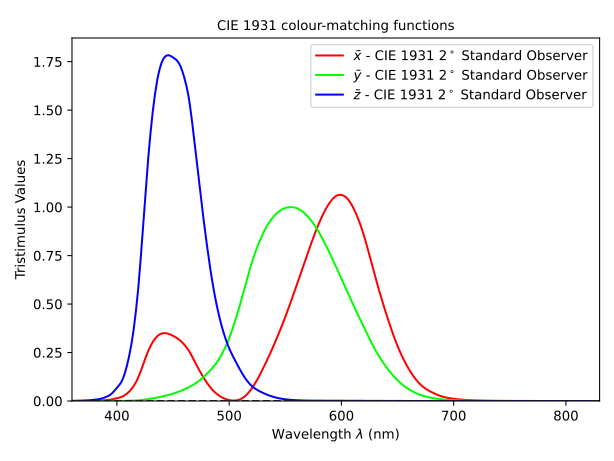
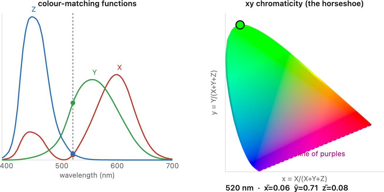
In a color-matching experiment, an observer views a test light beside a mixture of three fixed primaries. The primary amounts required for a match define its tristimulus coordinates. Some stimuli cannot be matched with nonnegative amounts: adding a primary to the test side is recorded as a negative amount on the mixture side. Repeating the experiment across wavelength gives the matching functions for those primaries. Wright and Guild used different primaries, and the CIE converted both data sets to three common monochromatic primaries at 700 nm, 546.1 nm and 435.8 nm Fairman, Brill & Hemmendinger 1997. The last two are emission lines of mercury, which any laboratory could reproduce exactly. The red was placed at 700 nm because in that part of the spectrum the hue hardly changes with wavelength, so a small error in setting it hardly changes the match. Spreading the three primaries far apart also keeps them well separated in cone response, the red and green especially, so the matching system is well conditioned.
The CIE 1931 standard transforms the measured matching functions to imaginary XYZ primaries. These are coordinate axes, not three lamps. The transformation makes all three XYZ matching functions nonnegative and makes $\bar y(\lambda)$ equal to the standard photopic luminous-efficiency function. For a spectral stimulus $E(\lambda)$,
The normalization $k$ determines the scale. For relative tristimulus values, choose it so the reference white has $Y=1$ (or explicitly $100$). For spectral radiance in physical units, the photometric conversion gives $Y$ in cd/m², with a factor approximately 683 lm/W and consistent wavelength units. Relative $Y=1$ is not one cd/m². Neither version of luminance is a full prediction of perceived brightness.
For sampled spectra, include bin widths:
XYZ = [0, 0, 0]
for each wavelength bin i:
    XYZ += k * E[i] * [xbar[i], ybar[i], zbar[i]] * delta_lambda[i]
Use tables for the intended observer and field size. The CIE 1931 two-degree tables specify one standard observer, not every individual’s cone sensitivities.
LMS coordinates can be defined as a linear transform of XYZ for a chosen colorimetric observer. That does not make modern physiological cone fundamentals an exact transform of the older 1931 observer. For example, the Hunt–Pointer–Estévez transform used in appearance models is
These model coordinates should not be substituted silently for measured cone excitations or a different normalization of cone fundamentals.
XYZ, a compatible LMS system, and linear RGB are different coordinates for a fixed observer’s three-dimensional color matches. Nonlinear RGB encodings and perceptual spaces add specified nonlinear transforms. A real camera’s raw measurements usually require an approximate color correction; an appearance model also needs viewing conditions.
A reference chart used in color characterization. Its patches sample a useful set of surface colors but do not prove accurate reproduction of every spectrum. See Chapter 45.16, Datasets.
The negative-primary case is easiest to understand at the apparatus. Suppose a saturated test cannot be matched by adding any nonnegative mixture of the three primary lamps. Move some red primary light to the test side, then adjust green and blue on the matching side until the fields agree. The recorded red coefficient of the original test is negative because that red was added to the opposite side of the equality. No lamp emits negative light. Linearity lets us subtract its contribution algebraically.
Repeat the match with narrow-band test lights across wavelength. The three settings at each wavelength form the color-matching functions. A broad spectrum can then be treated as a sum of these narrow-band contributions, which is why the integral above predicts its tristimulus coordinates. Transforming those coordinates to XYZ changes the coordinate system; it does not require building three imaginary lamps. A monitor illustration can show the controls and equations, but its own primaries limit which test spectra and matches it can physically reproduce.
One might wish that color technology had started with LMS: its axes have a direct interpretation in terms of the receptors. Later measurements of cone photopigments and the development of cone fundamentals made that interpretation much more accessible [@bowmaker-dartnall-1980; @stockman-sharpe-2000]. By then XYZ was already embedded in instruments, specifications, and device characterization. Replacing the common reference would have imposed a compatibility cost on all of them. XYZ also supplies a convenient luminance coordinate and nonnegative matching functions. Its persistence is therefore understandable even though its imaginary primaries and experimental origins make it harder to explain.
Keep the historical argument separate from the observer model. Linear coordinate changes preserve the matches of a fixed observer. A later physiological observer can differ from the 1931 standard; adopting it is not merely renaming the older coordinates. We can explain why XYZ stayed in use without claiming that every modern cone fundamental is an exact transform of the 1931 tables.
4.1.4 Chromaticity diagram⧉
For $X+Y+Z>0$, define
These coordinates discard scale: doubling the light leaves $x,y$ unchanged. Black has undefined chromaticity. Given $xyY$ with $y>0$, recover $X=xY/y$ and $Z=(1-x-y)Y/y$. Thus chromaticity plus luminance specifies the original tristimulus values; chromaticity alone does not.
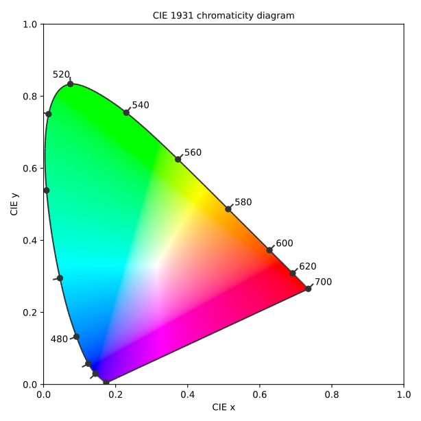
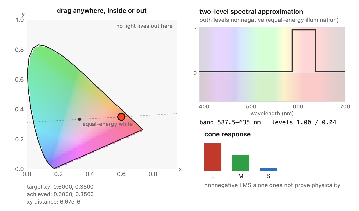
Monochromatic lights trace the spectral locus. Nonnegative mixtures lie in its convex hull, closed by the line of purples. The reference white is a selected point within this region, not an intrinsic center of the diagram. Euclidean distance in $xy$ is not a perceptual color difference.
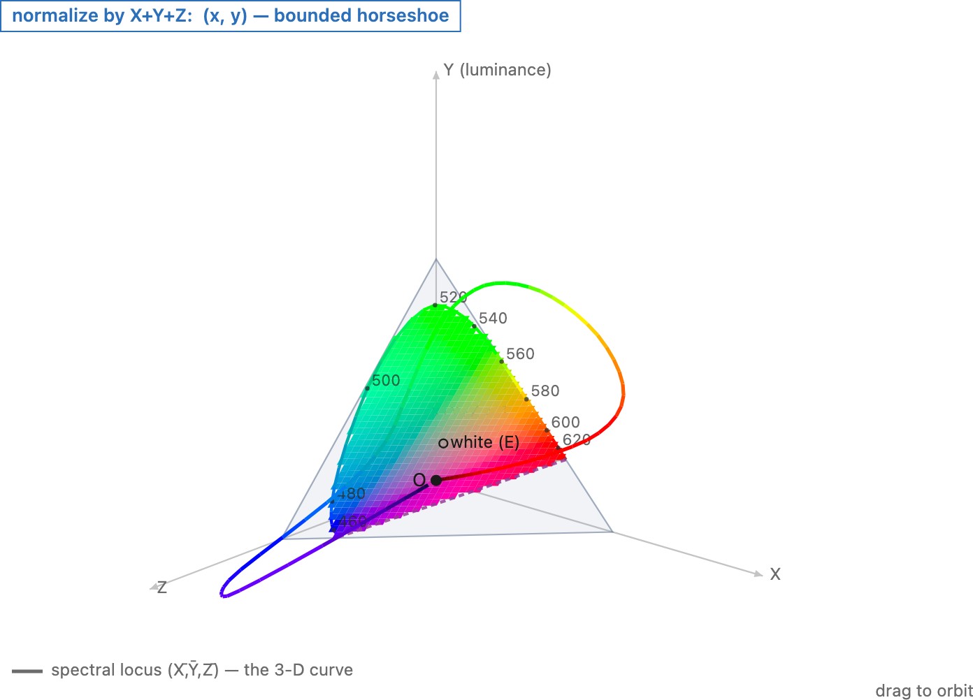
Geometrically, nonnegative spectra project to a cone of realizable tristimulus values Koenderink, Color for the Sciences. Normalizing by $X+Y+Z$ intersects each nonzero ray with a plane. Normalizing by another linear quantity gives a different cross-section. Although the underlying three-dimensional coordinates are related linearly, the normalized two-dimensional coordinates are related projectively.
MacLeod–Boynton chromaticity MacLeod & Boynton, cone-excitation chromaticity diagram (1979) uses cone fundamentals scaled so their L and M components sum to the luminance function. It plots $l=L/(L+M)$ and $s=S/(L+M)$. To interpret a horizontal displacement as an L–M trade at fixed luminance, hold the omitted scale $L+M$ fixed. The coordinates themselves do not force all plotted stimuli to have equal luminance, just as $xy$ does not.
A positive XYZ or LMS triple need not be physically realizable: positivity of three projections is weaker than existence of a nonnegative spectrum producing them. Reflectance introduces further constraints, since it must lie between zero and one under a specified illuminant. Do not confuse this surface-color problem with unconstrained emission.
Why divide by the sum rather than by luminance alone? Dividing by $Y$ is an appealing choice when the goal is to separate luminance from color, but coordinates such as $X/Y$ can become very large when $Y$ is small compared with another component. By dividing nonnegative XYZ coordinates by their sum, we instead put each normalized component between zero and one and make the three sum to one. The resulting diagram is bounded. This is a practical benefit of the chosen normalization, not a statement that its distances are perceptually uniform. Figure 4.1.8 makes the choice visible as a change of slicing plane.
The curved locus also has a physical origin. Sweep a monochromatic test through wavelength. At each setting its position comes from the three matching-function values at that wavelength, normalized by their sum. Those values vary together along the sensitivity curves, so the plotted point follows a curve rather than the sides of a triangle. Mixtures fill the convex region determined by that locus. The diagram's outline reflects the observer's spectral sensitivities; it is not an arbitrary shape chosen for a plotting convention.
4.1.5 Keeping track of what the numbers mean⧉
An array needs more than a label saying “RGB.” Record its primaries, transfer function, white reference, numeric range, and whether it represents scene light or a rendered image. Relative XYZ also needs its normalization. A camera-native RGB array needs a camera characterization.
Before a transform, check these assumptions against its input. A matrix defined for linear RGB cannot consume sRGB-encoded samples directly. Assigning a profile declares how existing numbers should be interpreted; converting to another profile changes the numbers to preserve the intended color. White adaptation changes a reference condition and must not be applied twice.
I find this bookkeeping more troublesome than most of the individual equations. Several independent choices travel under one name such as “sRGB,” and applications often hide which choices they made. Explicit metadata and a few labeled intermediate arrays are more useful than guessing from whether the picture looks plausible.
Treat a color transform like a units check. A matrix labeled as taking linear Rec. 709 RGB to XYZ cannot be fed the encoded samples read from an sRGB image. A value labeled Y′ is luma, so substituting it for linear luminance in a physical-light calculation changes the problem. A transform expecting a D65 reference cannot silently be given D50-relative coordinates. Writing the encoding and white reference next to an intermediate array makes these errors visible before the picture is displayed.
There are two kinds of difficulty here. Some come from the measurement: three responses do not determine a spectrum, and the same surface sends different light under different illumination. Others come from conventions maintained across decades, such as print workflows using D50, common display spaces using D65, and the name sRGB covering both primaries and a transfer function. Separating the physical ambiguity from the bookkeeping helps identify what a better calibration can solve and what merely needs an explicit conversion.
A cleaner interface would separate the measurement of the incoming light from the choice of how a particular device should reproduce it. The measurement would identify its observer and normalization; the rendering would specify the viewing conditions, output device, and intended appearance. Color management tries to provide this separation through documented profiles and a common connection space (Chapter 4.8, Recap: the full color pipeline, color management and ICC). It has to work with existing representations, though. A name such as sRGB specifies primaries, a white reference, and an encoding together. Separating those choices remains work for the programmer. The type annotations make that separation explicit on the page.
4.1.6 Linear RGB⧉
LMS and XYZ are analysis spectra, built to measure color. To store and reproduce it we use the RGB family, and the standard member is sRGB (Stokes et al. 1996 (sRGB)), whose primaries are the Rec. 709 primaries under the D65 white point. In linear light, sRGB and XYZ are one $3\times3$ apart. The forward matrix takes a measured color into linear sRGB,
and its inverse recovers XYZ,
The coefficients shown are rounded. Apply them to linear values; a typical sRGB file must first be decoded. The middle row of the RGB-to-XYZ matrix gives relative luminance. Applying those weights to encoded components gives luma, which is neither luminance nor generally the encoding of luminance.
Negative RGB components indicate a target outside the positive cone spanned by these primaries. Components above one exceed the chosen reference range; they can represent greater intensity at an otherwise reproducible chromaticity. Floating-point scene-linear images often retain such values. Clipping to $[0,1]$ is an output decision that can change hue and discard highlight information.
Recap: big lessons of this chapter
Sensitivity curves measure a spectrum; emission primaries construct one. Reusing the sensitivity curves as primaries and the measured responses as weights generally gives the wrong color. Calibrate how each primary stimulates the observer, then solve for its weight.
XYZ, a compatible LMS system, and linear RGB are different coordinates for a fixed observer’s three-dimensional color matches. Nonlinear RGB encodings and perceptual spaces add specified nonlinear transforms. A real camera’s raw measurements usually require an approximate color correction; an appearance model also needs viewing conditions.