21.3 Inpainting using millions of photographs⧉
The preceding chapters filled holes by propagating boundaries or copying patches from the same image. Hays and Efros's Scene Completion Hays & Efros 2007 expands the source to millions of other photographs: retrieve a compatible scene and borrow a region from it. The retrieval and collection methods are developed later in Chapter 28.2, Retrieval and Chapter 28.1, Photo Mosaics. Here the database serves a concrete editing task and makes an instructive comparison with learned generative inpainting.
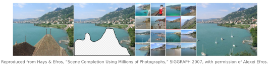
The data is the prior. A learned inpainting model encodes "what scenes look like" in its weights; Scene Completion encodes the same knowledge in the collection itself: no parametric model, no training, just a large enough pile of real photographs and a fast nearest-neighbor search. Scale does the work a model would otherwise do: at a few million images, the database has effectively already seen a plausible completion of almost any ordinary scene, and the algorithm's only job is to find it and paste it in cleanly. This is the wager Chapter 28.8, Pix 2 GPS and Chapter 28.9, Personalized priors each make in their own domain (the collection is the model), and the whole part is variations on it. The reason to state it loudly here is the contrast it sets up: when diffusion inpainting later puts the prior back into weights, you will be able to see exactly what was traded away.
21.3.1 Why self-similar inpainting isn't enough⧉
Classical inpainting copies patches from within the same image. The texture-synthesis lineage, beginning with Efros & Leung (1999) and then Criminisi et al. (2004), grows the known texture inward across the hole, matching each new patch against the surrounding image. For a small hole in homogeneous texture this is exactly right: a scratch across a brick wall, a speck on a lawn, a removed power line against open sky all close seamlessly, because the pixels that belong in the hole genuinely are present nearby. The image is its own database, and for these cases it is a sufficient one.
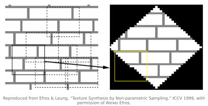
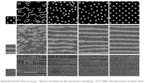
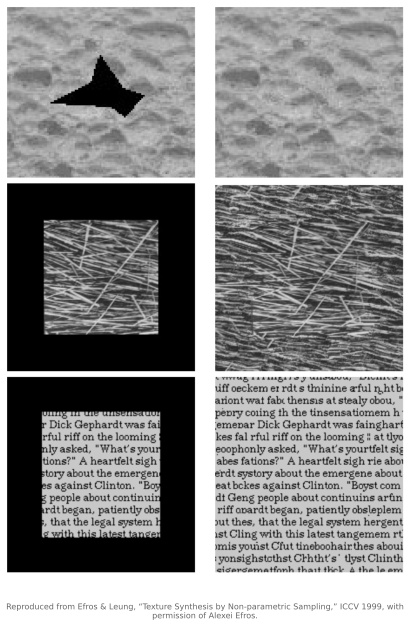
The method can fail when the hole requires structure that does not recur elsewhere in the image. Remove a person standing in front of a building and the missing region is not more of a visible texture; it is the part of the building the person was occluding, content that the image simply does not contain. No amount of copying from the visible pixels can invent the window, the doorway, the horizon line that belonged behind the subject. Self-similar synthesis can only ever extend what is there; it cannot supply what is absent.
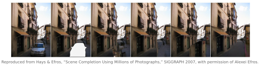
The reframing is the whole idea. A plausible replacement may already exist: they are just in a different photograph, of a similar scene, taken by someone else. A thousand other people have photographed a building, a beach, a street corner, a mountain ridge like yours. So stop treating inpainting as synthesis ("invent the missing pixels from this image") and treat it as retrieval-and-paste ("find a real photograph whose content fits the hole, and borrow it"). The image's own pixels were the wrong database; the right one is the rest of the photographed world.
21.3.2 Scene completion from a huge database⧉
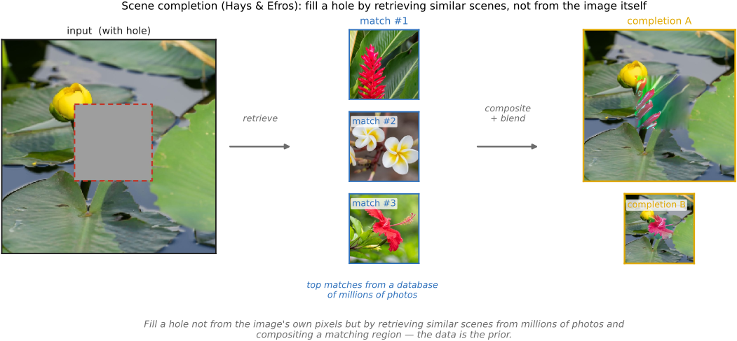
The pipeline has three moves: retrieve, align-and-cut, blend (Figure 21.3.7). The first is the heart of it. Describe the image around the hole with a scene-level descriptor, here GIST (Oliva & Torralba, 2001), a coarse summary of the scene's spatial layout (horizon, openness, dominant structures), deliberately blind to fine detail. Then search a database of millions of photographs for scenes whose GIST, computed on the context surrounding the hole, matches the query (Chapter 28.2, Retrieval). You are not looking for the same object; you are looking for the same kind of scene: a matching horizon, a compatible scene type, a plausible global structure into which the borrowed patch can slot. Adding a coarse color match to GIST tightens the candidates to scenes that will also composite without a jarring tonal jump.
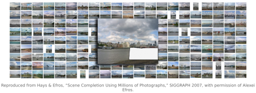
For each good match, the missing content must be cut out and pasted in. The matched photograph is aligned to the query, the region covering the hole is identified, and the algorithm chooses where exactly to splice, finding a seam through the overlap zone where the borrowed patch and the original agree most closely. That seam is a graph cut (Kwatra et al., 2003): the optimal boundary is the minimum-cost cut of a graph whose edge weights penalize visible mismatch, so the splice line threads through pixels where the two images already look alike. Then Poisson blending (Pérez et al., 2003) reconciles the residual difference, solving for an image whose gradients match the borrowed patch's interior while its values match the original at the boundary, so boundary color and brightness agree, although incompatible structure or texture can still reveal the edit (Chapter 10.8, Poisson image editing / Chapter 20.3, Blending). Cut where the images agree, then blend away what disagreement remains.
The third move is a stance: offer several answers, not one. Because many database scenes match the context, there is no single correct fill: a removed building could plausibly be replaced by any compatible building, a missing field by any compatible field. Rather than commit to one, Scene Completion composites a selection of matches and presents several plausible completions side by side (Figure 21.3.7). Surfacing the genuine ambiguity is part of the result, and it is the same stance as the heatmap-not-a-pin output of Chapter 28.8, Pix 2 GPS: when the data admits many answers, report many answers.
21.3.3 The data is the prior, and its modern opposite⧉
Step back from the mechanics and the philosophical claim is sharp. Scene Completion uses no learned parametric model of the missing scene. Its scene descriptors, matching criteria, and blending objective still encode design assumptions. What "scenes look like" is not stored in model weights; it is simply present, distributed across the million photographs, and read out at query time by nearest-neighbor search. The prior is the database. This is why the result improves as the corpus grows, and why Hays and Efros found a step-change in quality between tens of thousands of images and millions: at small scale the nearest match is a poor fit and the seam betrays it, while at millions the nearest match is genuinely of a scene like yours and the composite is convincing. Scale is doing the work a learned prior would otherwise do: the same wager Chapter 28.8, Pix 2 GPS, makes for geolocation and Chapter 28.9, Personalized priors, makes for a single subject.
The contrast with model-based inpainting (forward-referenced to the diffusion sections) is the cleanest way to see what data-as-prior buys and costs. Modern diffusion inpainting bakes the prior into network weights and synthesizes the fill by iteratively denoising new, coherent pixels conditioned on the surrounding context, inventing content that was never photographed. Data-as-prior versus weights-as-prior: the two have opposite failure modes. Scene Completion borrows a real photograph, so its pixels are always individually plausible, but it may import the wrong specifics, a building of the right type but visibly the wrong building, complete with a stranger's window boxes. Diffusion invents coherent pixels tailored to this image, but they are a confident fabrication, plausible-looking content that no camera ever recorded. The retrieved pixels come from a real source photograph but need not describe the hidden scene; generated pixels likewise provide no direct measurement of it. The task is the same, but the assumptions differ. Scene Completion is useful to meet first because it makes the data-driven prior explicit, the pole against which the model-driven era defines itself.
Recap: big lessons of this chapter
The data is the prior. A learned inpainting model encodes "what scenes look like" in its weights; Scene Completion encodes the same knowledge in the collection itself: no parametric model, no training, just a large enough pile of real photographs and a fast nearest-neighbor search. Scale does the work a model would otherwise do: at a few million images, the database has effectively already seen a plausible completion of almost any ordinary scene, and the algorithm's only job is to find it and paste it in cleanly. This is the wager Chapter 28.8, Pix 2 GPS and Chapter 28.9, Personalized priors each make in their own domain (the collection is the model), and the whole part is variations on it. The reason to state it loudly here is the contrast it sets up: when diffusion inpainting later puts the prior back into weights, you will be able to see exactly what was traded away.