33.0 COMPUTATIONAL OPTICS AND CODED IMAGING⧉
Two lessons have run through everything so far, and this part is built on top of both. The first is image formation: a sensor pixel does not see a point of the world, it sees a cone of light rays, and it reports their integral, one number that sums everything that crossed the aperture and landed there. The second is ray selection: the optics decides which rays land on which pixel. A pinhole selects one thin pencil per pixel; a lens gathers a whole cone and converges it; focus is just the name for getting that selection right. Put the two together and a camera is a machine that, pixel by pixel, picks a set of rays and adds them up.
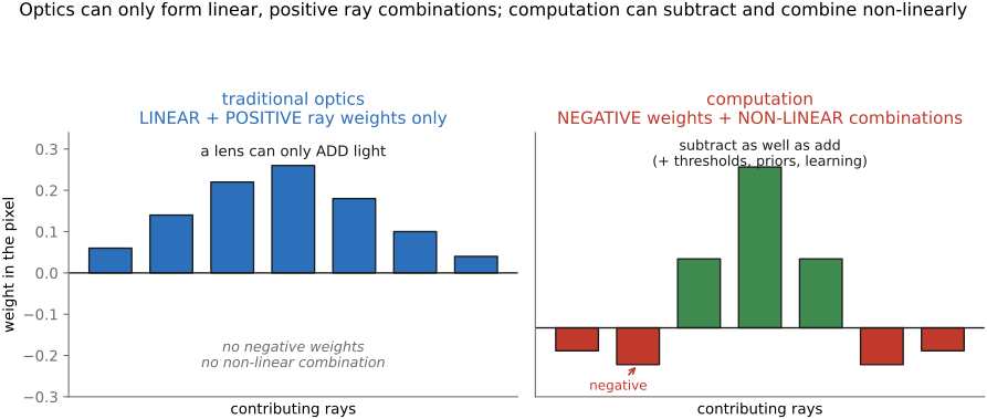
The constraint is simple. In the incoherent radiance model used here, fixed passive optics form linear, nonnegative combinations of incoming radiance. It can gather light and sum it, weight some directions more than others, even throw some away, but it cannot subtract one ray from another, and it cannot make a pixel a non-linear function of its rays. Glass only adds light; it does not negate it. The linear sensor signal is therefore a weighted sum with nonnegative weights, not necessarily normalized to an average, and that single restriction bounds what optics alone can do.
Coded imaging is the idea of letting optics and computation together decide the ray combination behind each final pixel. The move is to split image formation into two stages. The optics no longer has to make the picture; it only has to encode the scene's rays into an intermediate measurement, a code that is not yet a photograph, often a deliberately scrambled or blurred image. Then computation decodes that measurement into the final image. The name is borrowed from communication theory on purpose: the optics is an encoder, the sensor records the code, and the algorithm is the decoder that turns it back into a picture. We are after the same goal as a good communication code: capture the information now and reconstruct it faithfully later.
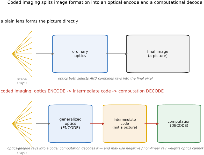
The reason to bother is that the decoder is not bound by the optics' limits. Computation can give rays negative weights. That is exactly what deblurring does when it subtracts the blurred neighbors back out of a pixel, and it can combine them non-linearly, applying thresholds, priors, or a learned reconstruction. The optics is stuck with linear, positive averages; the computation is not, and coded imaging is the discipline of designing the optical encoder and the computational decoder together so the pair captures and recovers more than either could alone.
Two goals organize the whole part. The first is better end-to-end capture of information, and with it resilience to noise. If the optics encodes the scene with a blur that is invertible, one that retains useful contrast over a specified frequency band, then regularized reconstruction can recover useful detail over a greater operating range. Invertibility alone does not guarantee stable recovery in noise. The encoder's job is to choose a code that survives the trip through the sensor (and its noise) with the information intact; the decoder's job is to invert it. The second goal is choosing imaging parameters after the shutter has closed. If the intermediate code captures more than any one picture needs, the computation can form many pictures from it, and decide the parameters a posteriori, most famously the focus, recomputed at will from a single capture (the refocusing of Part 31, Light fields and plenoptic cameras), but the same logic reaches aperture, viewpoint, and more.
The part runs from the canonical example outward to the general machinery and the hardware. Chapter 33.1, Wavefront coding is the textbook first instance of the encode→decode story: a cubic phase plate in the pupil encodes the scene with a blur that varies little over a designed defocus range, and one fixed deconvolution decodes it into an image with a greatly extended depth of field, from one capture, subject to its depth range, sampling, and noise limits. Chapter 33.2, Compressive sensing is the purest statement of the thesis: the sensor takes far fewer measurements than there are unknowns, each a coded linear combination of the scene, and computation recovers the whole signal by exploiting sparsity (the single-pixel camera is its emblem). Chapter 33.3, Coded aperture puts a patterned amplitude mask in the lens, encoding depth into the blur so it can be read back out and inverted. Optical modulators, such as DMDs and liquid-crystal panels, are the programmable hardware that does the coding on the fly, the active cousins of the fixed masks. And Exotic / advanced optics pushes the idea to its limit, replacing the lens entirely with a mask or diffuser and reconstructing the image purely by computation. A closing chapter collects exotic optics, including GRIN lenses, metalenses, and non-linear optics, where the wavefront is shaped in other ways.
One sentence summarizes the part: a conventional camera forms the picture in glass, with linear positive ray sums; coded imaging lets the glass merely encode the rays and hands the picture to computation, which can use signed and nonlinear reconstruction while remaining limited by the information and noise in the measurements. Wavefront coding is where we start, because it is the cleanest place to watch a deliberate blur become a feature rather than a flaw.
Contents of this part
- 33.1 Wavefront coding
- 33.1.1 Why you cannot just deblur defocus
- 33.1.2 The fix: re-engineer the blur
- 33.1.3 The cubic phase plate
- 33.1.4 The depth-invariant PSF and a single deconvolution
- 33.1.5 What it costs
- 33.1.6 Where it sits
- 33.2 Compressive sensing
- 33.2.1 Sub-Nyquist: fewer measurements than unknowns
- 33.2.2 Two ingredients: incoherent measurements and sparsity
- 33.2.3 Recovery by $\ell_1$: the geometry of basis pursuit
- 33.2.4 Why it works: the restricted isometry property, intuitively
- 33.2.5 The single-pixel camera
- 33.2.6 Where compressive sensing wins, and where it does not
- 33.3 Coded aperture
- 33.3.1 The bad forward operator of a clear aperture
- 33.3.2 A mask designed for a flat, zero-free spectrum
- 33.3.3 One shot, two outputs: depth and an all-in-focus image
- 33.3.4 The design criterion: which pattern?
- 33.3.5 Coded-aperture pairs: splitting the trade across two shots
- 33.3.6 Heterodyning the light field: dappled photography
- 33.3.7 Where it sits
- 33.4 Phase-coded apertures
- 33.4.1 A reminder on wavefront coding
- 33.4.2 Focus sweep
- 33.4.3 The lattice-focal lens
- 33.4.4 Where it sits
- 33.5 Code in time (phase, amplitude)
- 33.5.1 Why ordinary motion blur is (almost) unrecoverable
- 33.5.2 The flutter shutter: chop the exposure into a code
- 33.5.3 The decode: one deconvolution, a sharp moving object
- 33.5.4 Amplitude in time, and phase in time
- 33.5.5 Coded strobing, temporal multiplexing, and compressive video
- 33.5.6 Motion-invariant photography
- 33.5.7 Where it sits
- 33.6 Theoretical analysis of imaging systems in the 4D light field Fourier domain
- 33.6.1 The light field's spectrum, and the one move that explains everything
- 33.6.2 Every camera is a different slice
- 33.6.3 Putting cameras on one footing: the Bayesian comparison
- 33.6.4 The dimensionality gap: most of the 4-D spectrum is afocal
- 33.6.5 The lattice-focal lens: tiling the wedge
- 33.6.6 The upper bound, and the gap we have not closed
- 33.6.7 From cameras to light transport: the same spectral lens
- 33.6.8 Where this leaves the part
- 33.7 End-to-end optimization
- 33.8 Fourier optics
- 33.8.1 Light as a wave: amplitude, phase, and what "coherent" means
- 33.8.2 Diffraction is a Fourier transform
- 33.8.3 A lens computes a Fourier transform
- 33.8.4 The pupil function is the transfer function
- 33.8.5 The diffraction limit
- 33.8.6 Aberrations are pupil phase
- 33.8.7 Every code in this part is a choice of pupil
- 33.8.8 Fourier ptychography: synthesizing a bigger pupil
- 33.9 Exotic / advanced optics
- 33.9.1 Lensless imaging
- 33.9.2 GRIN
- 33.9.3 Metalenses and advanced crazy optics à la Barbastathis (coherent though)
- 33.9.4 Non-linear optics
- 33.10 Optical modulators (spatial light modulators): DMD and LCD/LCoS