BookNotesSlidesP-sets Syllabusdraft · v0.2.49.1
💬Comments welcome. To leave a note, select any text and click the note / highlight button that pops up — or open the panel with the tab at the top-right (‹). Notes are visible only inside our private review group.
Computational Photography, an AI-powered Slopendium — 20 Field of view extension and panorama stitching
expand to📖 Full book outline1 parts · 5 chapters · 26 sections · 25 figures embedded · 16 placeholders · double-click a figure to enlarge
▸Part 20 FIELD OF VIEW EXTENSION AND PANORAMA STITCHING⧉
<!--uid: field-of-view-extension-and-panorama-stitching-->
▸20.1 Manual panorama stitching from multiple views⧉
fig-pano-rotate-vs-translate
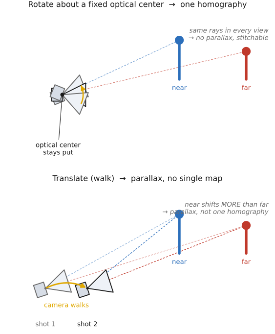
fig-pano-rotate-vs-translate · pure camera rotation about a fixed center (views related by one homography) vs camera translation (parallax, no single map) 🟨
fig-depth-cancels-ray
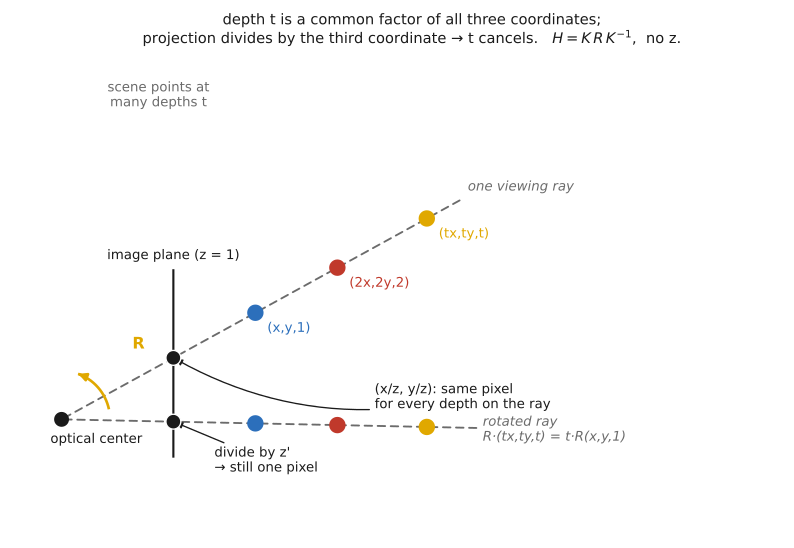
fig-depth-cancels-ray · points at different depths along one ray collapsing to a single pixel after rotation and reprojection — depth drops out of the view-to-view map 🟨
⬜ figure not yet created
`fig-pinhole-divide-by-z` (3D point $(x,y,z)$ → image $(x/z,y/z)$: projection = divide by depth) fig-pinhole-divide-by-z
fig-homography-quad
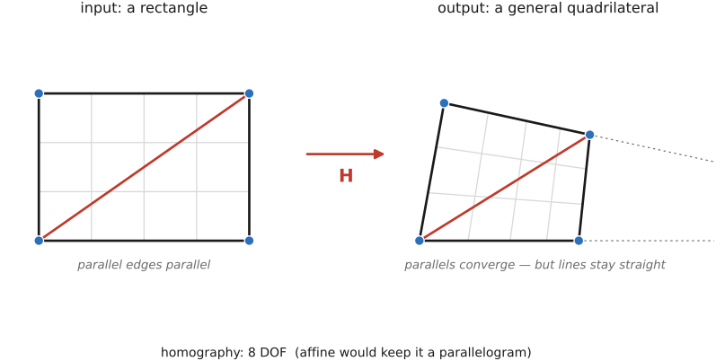
fig-homography-quad · a homography sending a rectangle to a general quadrilateral, keeping lines straight while letting parallels converge (8 DOF; affine would keep a parallelogram) 🟨
⬜ figure not yet created
`fig-homog-coords-1d` (1D homogeneous coords: point $x$ ↔ ray $(x,1)$ fig-homog-coords-1d
fig-fundamental-matrix
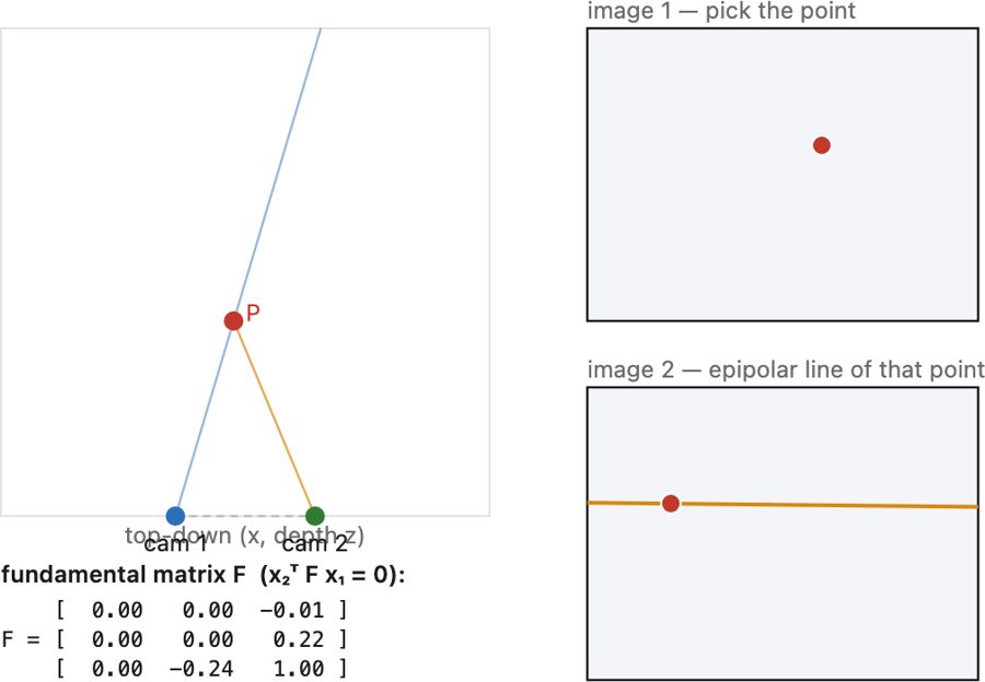
fig-fundamental-matrix · **interactive** epipolar/fundamental-matrix demo (image-pair view, complements the 3-D `fig-epipolar-line`): pick a point in image 1 (u₁,v₁), slide the depth of P along its back-projection ray, and watch P's image slide along the **epipolar line** drawn in image 2; a top-down panel shows the triangulation; camera-2 **baseline + toe-in** sliders change the relative pose; the **fundamental matrix F** (x₂ᵀ F x₁ = 0) is computed live. ✅
⬜ figure not yet created
`fig-pano-warp-to-reference` (pick one image as reference fig-pano-warp-to-reference
fig-pano-4clicks
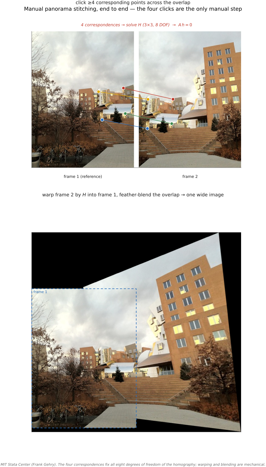
fig-pano-4clicks · the manual stitching pipeline: click four correspondences across the overlap, solve $H$, warp, blend into one wide frame 🟨
fig-doc-flatten
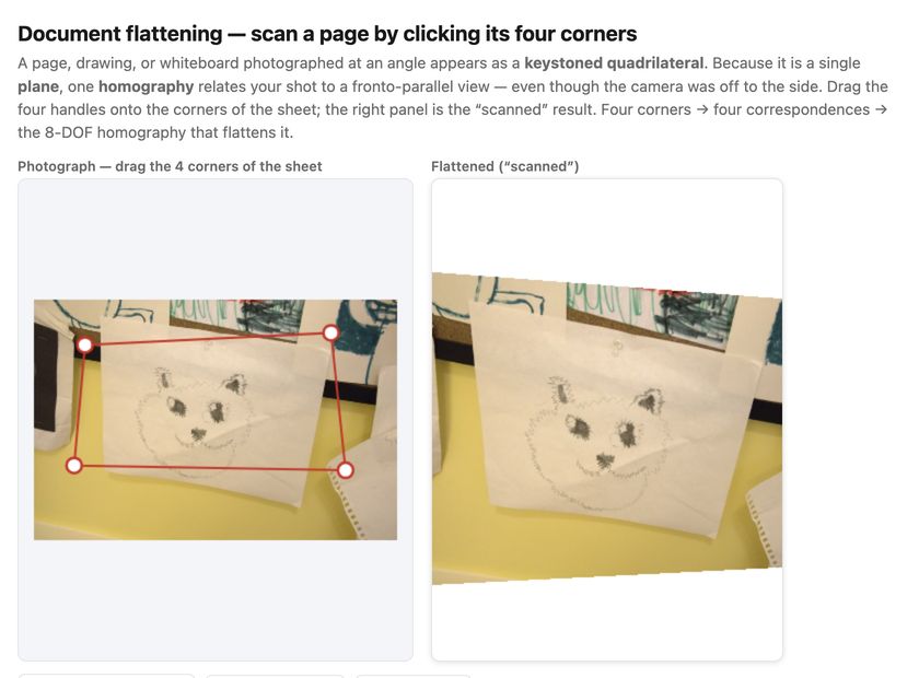
fig-doc-flatten · **interactive** document flattening (10.4): drag the four corners of a page/drawing photographed at an angle → fronto-parallel "scan" via the recovered homography (planar-scene case); three real children's-drawing photos (cat sketch, lion on black paper, framed dolphin) + upload ✅
💡 **Big lesson (L11.2 · Capture the full set, decide later):** *the move that drives this whole part is — instead of committing one capture parameter at the instant of exposure, **record the whole set and choose afterward**.* A panorama defers your **field of view**: shoot several overlapping frames now, decide the final framing/crop of the wide view later. It is the same move as exposure bracketing → HDR (capture all exposures), focus stacks (all focal planes), and burst imaging (every instant). The cost is data and a harder reconstruction (alignment + blending); the payoff is taking an irreversible decision *out* of the moment of capture. (Registered in [[Big Lessons]] as **L11.2** — *first appears* with light-field/plenoptic cameras, but it is the **spine of this part** and surfaces in every section here; one-line callbacks at HDR, focus stacks, and panoramas.)
A panorama is the oldest computational-photography trick: a single shot can't see wide enough, so take **several overlapping photos** and stitch them into one wide image. The deep question is *what relates two overlapping photos of the same scene?* — and the surprisingly clean answer (no 3D, no depth) is what makes stitching a tractable problem rather than a full reconstruction. This chapter does the geometry by hand; the **manual** version asks the user to click the correspondences, and the [[#Automatic panorama stitching from multiple views and feature matching|next chapter]] automates them.
equations
pinhole projection $(x,y,z)\mapsto(x/z,\,y/z)$ (project = divide by depth)
homography $\mathbf{x}' \simeq H\mathbf{x}$ with $H\in\mathbb{R}^{3\times3}$, **8 DOF** (defined up to scale, $H\sim kH$)
pure-rotation view-to-view map $H = K R K^{-1}$ — **independent of depth**
for the calibrated/normalized case $H = R$ acting on rays $(x,y,1)$
the per-point divide $\big(x',y'\big)=\big(\tfrac{a x+by+c}{gx+hy+i},\,\tfrac{dx+ey+f}{gx+hy+i}\big)$
the linear system $A\mathbf{h}=\mathbf{0}$ (each correspondence → 2 rows
4 correspondences → 8 equations in 8 free unknowns).
▸20.2 Automatic panorama stitching from multiple views and feature matching⧉
fig-feature-pipeline
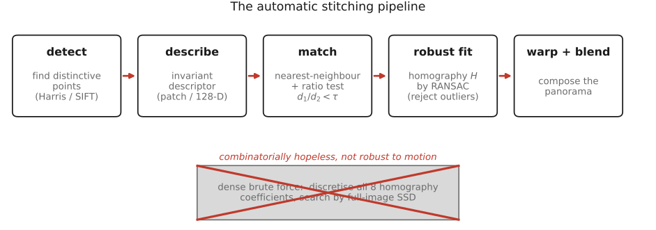
fig-feature-pipeline · the detect → describe → match → robust-fit feature pipeline that automates stitching, with the abandoned dense-SSD search crossed out beside it 🟨
fig-corner-flat-edge
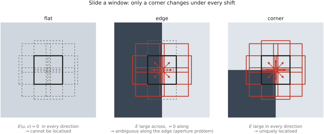
fig-corner-flat-edge · why corners are the best keypoints — only a corner's small window changes under a shift in every direction (flat / edge / corner columns, aperture problem) 🟨
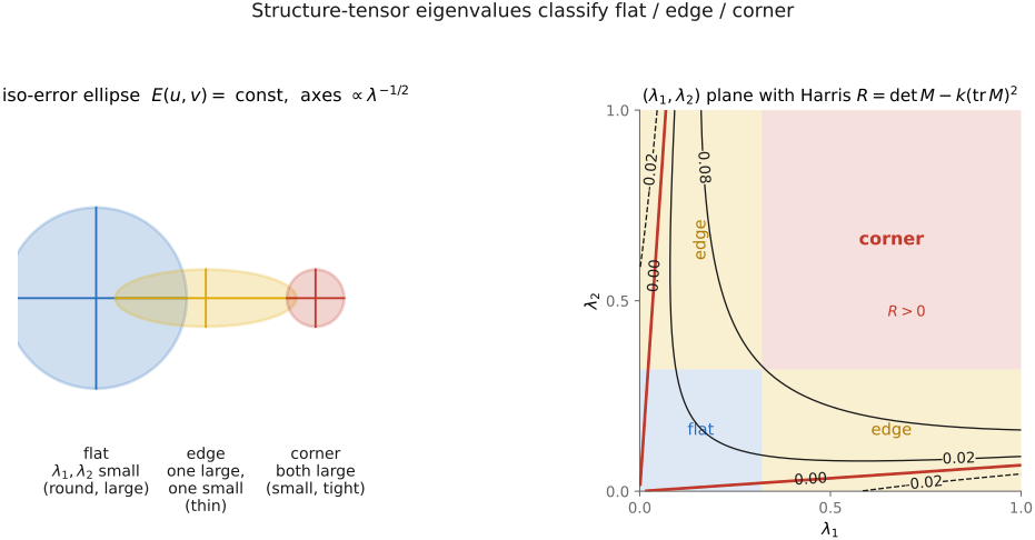
fig-harris-eigen-ellipse
fig-harris-eigen-ellipse · the structure tensor's eigenvalues linked to the flat / edge / corner classification and the sign of the Harris response $R=\det M-k(\operatorname{tr}M)^2$ 🟨
⬜ figure not yet created
axes $\propto\lambda^{-1/2}$
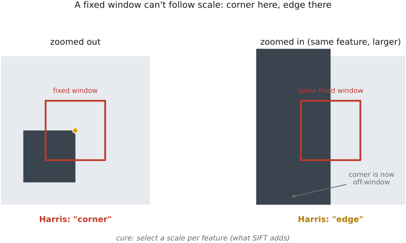
fig-harris-not-scale-invariant
fig-harris-not-scale-invariant · one scene corner classified "corner" at one scale and "edge" at another under a fixed window, motivating scale selection 🟨
⬜ figure not yet created
`fig-scale-space-bumps` (1D bumps of three widths blurred over a stack of Gaussians fig-scale-space-bumps
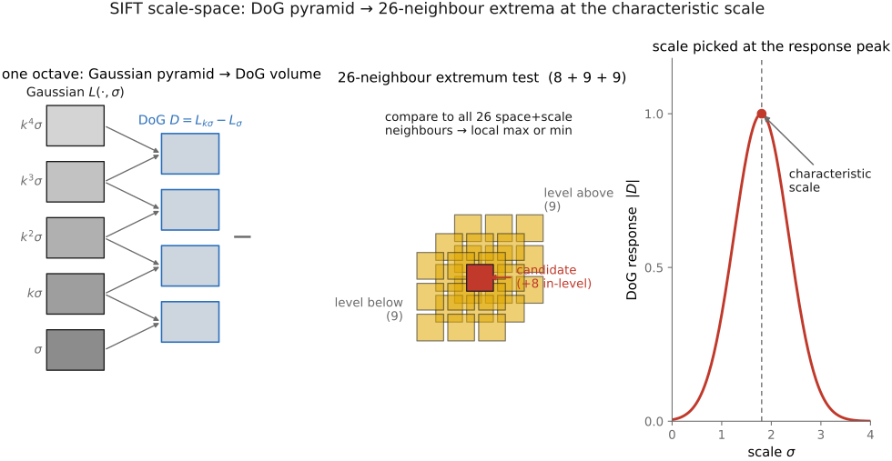
fig-dog-pyramid
fig-dog-pyramid · the Difference-of-Gaussians pyramid and the 26-neighbor space-and-scale extremum test that detects SIFT keypoints 🟨
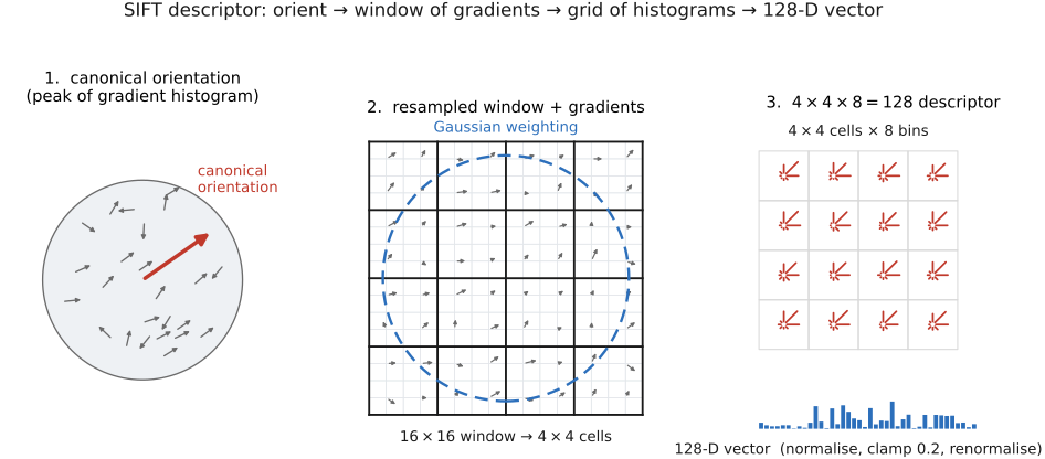
fig-sift-descriptor
fig-sift-descriptor · the $16\times16$ window → $4\times4$ grid of 8-bin orientation histograms → 128-D normalized vector that is the SIFT descriptor 🟨
⬜ figure not yet created
`fig-canonical-orientation` (gradient-orientation histogram of the patch fig-canonical-orientation
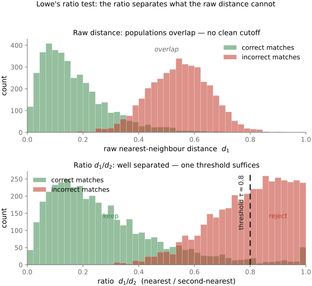
fig-ratio-test-histograms
fig-ratio-test-histograms · overlapping raw-distance histograms vs well-separated ratio $d_1/d_2$ histograms for correct/incorrect matches, showing why the ratio test discriminates 🟨
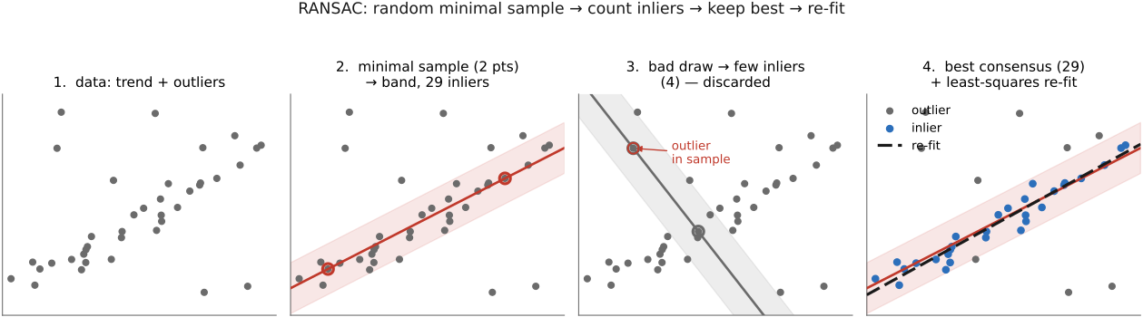
fig-ransac-line
fig-ransac-line · RANSAC's sample → fit → count-inliers → keep-best → re-fit loop on a toy line-fitting example, four panels 🟨
⬜ figure not yet created
`fig-ransac-pano-inliers` (a real overlap: matches colored — rejected-by-ratio-test, RANSAC outliers, inliers — and the resulting clean stitch) fig-ransac-pano-inliers
⬜ figure not yet created
`fig-ransac-iterations-graph` (probability-of-failure vs inlier fraction $w$, family of curves for $N=10,10^2,\dots,10^6$ iterations — the exponentials at work) fig-ransac-iterations-graph
The [[#Manual panorama stitching from multiple views|manual pipeline]] is complete except for one human step: someone clicked the corresponding points. That step is the bottleneck — slow, and impossible at scale (gigapixel mosaics, photo collections, video). This chapter replaces the clicks with **automatic feature matching**, which Durand's slides rightly call *"perhaps the most important innovation in computer vision and computational photography in the last twenty years"* — the same machinery powers 3D reconstruction, tracking, object recognition, retrieval, and robot navigation. We keep the homography solve from before; we only manufacture its inputs.
equations
window SSD under a shift $E(u,v)=\sum_{x,y} w(x,y)\,[I(x+u,y+v)-I(x,y)]^2$
**Taylor → quadratic form** $E(u,v)\approx \begin{psmallmatrix}u&v\end{psmallmatrix} M \begin{psmallmatrix}u\\ v\end{psmallmatrix}$ with the **structure tensor** $M=\sum w\begin{psmallmatrix}I_x^2&I_xI_y\\ I_xI_y&I_y^2\end{psmallmatrix}$
**Harris response** $R=\det M-k(\operatorname{tr}M)^2=\lambda_1\lambda_2-k(\lambda_1+\lambda_2)^2$ ($k\approx0.04$–$0.06$)
Shi–Tomasi $R=\min(\lambda_1,\lambda_2)$
**scale-space** $L(\cdot,\sigma)=G_\sigma*I$, **DoG** $D=L(\cdot,k\sigma)-L(\cdot,\sigma)\approx(k{-}1)\sigma^2\nabla^2 G*I$ (scale-normalized Laplacian)
**descriptor distance** SSD $d=\lVert \mathbf{f}_i-\mathbf{f}_j\rVert^2$
**ratio test** $d_1/d_2<\tau$ ($\tau\approx0.8$, $d_1\le d_2$ the two nearest neighbors)
**RANSAC inlier test** $\lVert \mathbf{x}_i'-H\mathbf{x}_i\rVert<\varepsilon$
probability a random $s$-sample is all-inlier $w^s$
**iteration count** $N=\dfrac{\log(1-p)}{\log(1-w^s)}$ (succeed with prob. $p$
inlier fraction $w$
sample size $s{=}4$ for a homography).
20.2.2 The feature pipeline, recalled⧉
▸20.3 Blending⧉
⬜ figure not yet created
`fig-blend-visible-seam` (a registered two-image mosaic with a hard photometric seam — exposure + white-balance + vignetting mismatch — the problem statement) fig-blend-visible-seam
⬜ figure not yet created
`fig-blend-feather-ghost` (single distance-weighted average → the same scene where small misregistration produces a doubled/ghosted edge and overall blur) fig-blend-feather-ghost
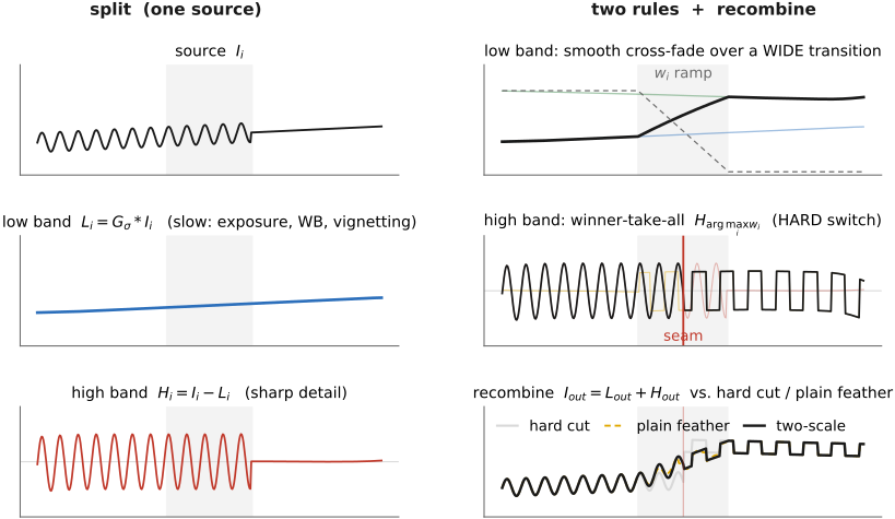
fig-blend-twoscale-split
fig-blend-twoscale-split · a source split into low and high bands, the low band blended smoothly and the high band composited winner-take-all, plus a hard-cut / feather / two-scale comparison 🟨
⬜ figure not yet created
`fig-blend-twoscale-result` (basic reprojection vs smooth blend vs two-scale, side by side — the slide-95/96 comparison) fig-blend-twoscale-result
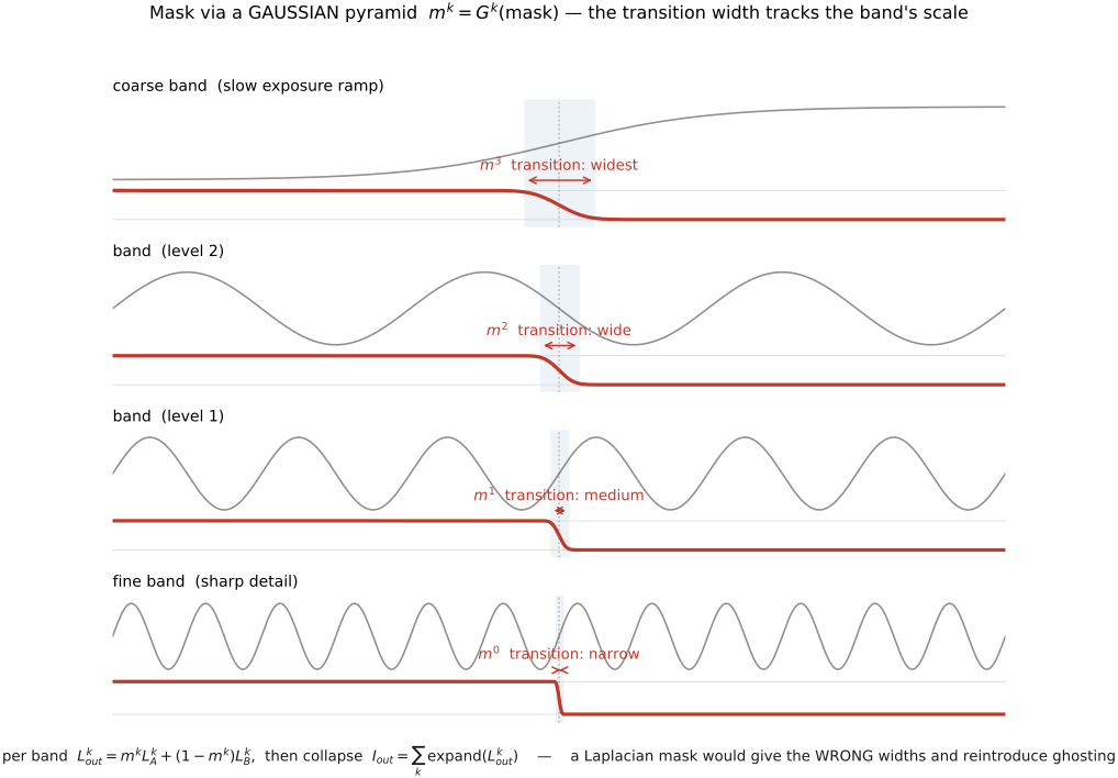
fig-blend-mask-pyramid
fig-blend-mask-pyramid · the blend mask decomposed by a Gaussian pyramid, the transition wide at coarse levels and sharp at fine levels, explaining why width tracks frequency band 🟨
⬜ figure not yet created
`fig-blend-laplacian-bands` (per-band blend $L^k_{out}=m^k L^k_A+(1-m^k)L^k_B$ then collapse → the seamless multiband result) fig-blend-laplacian-bands
fig-blend-poisson-vs-pyramid
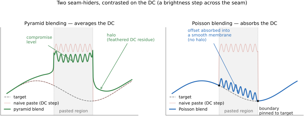
fig-blend-poisson-vs-pyramid · pyramid vs Poisson blending on a paste with a DC offset — the pyramid leaves a faint low-frequency halo, Poisson absorbs the offset into the boundary 🟨
fig-blend-seam-graphcut
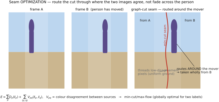
fig-blend-seam-graphcut · two overlapping frames with a moving person and the min-cut seam routed through low-disagreement pixels around the person, taking them entirely from one source 🟨
💡 **Big lesson (L6.3 · the eye cares about gradients, not absolute values):** a stitch seam is jarring not because the *average* brightnesses differ but because the **gradient is wrong right at the boundary** — a sudden jump the visual system reads as an edge that isn't in the scene. So the entire blending ladder is a sequence of ways to *fix the gradients at the seam*: smooth-blend the low frequencies so the jump is spread out (two-scale, multiband), or paste the gradients and solve for values so the jump is **absorbed into an invisible DC shift** (Poisson), or route the seam through pixels whose gradients already match so there is nothing to fix (graph cut). A constant brightness/color offset between two frames is **invisible once the boundary gradient is right** — exactly why gradient-domain blending works. (→ first appears in [[Poisson image editing]] — *the key idea*; recurs here as the organizing principle of stitch blending.)
equations
**feathering / alpha** $I_{out}(p)=\dfrac{\sum_i w_i(p)\,I_i(p)}{\sum_i w_i(p)}$ with $w_i$ a distance-to-boundary weight
**two-scale** — split $I_i=L_i+H_i$ ($L_i=G_\sigma * I_i$, $H_i=I_i-L_i$)
blend low band by feathering, high band winner-take-all $H_{out}(p)=H_{\arg\max_i w_i(p)}(p)$
**multiband / Laplacian** per band $L^k_{out}=m^k\,L^k_A+(1-m^k)\,L^k_B$ where $m^k$ is the **Gaussian-pyramid** level-$k$ of the mask, then collapse $\sum_k \mathrm{expand}(L^k_{out})$
**Poisson blend** $\displaystyle \min_f \iint_\Omega \lVert\nabla f - \mathbf v\rVert^2\ \text{s.t. } f|_{\partial\Omega}=I_{\text{target}}|_{\partial\Omega}$, Euler–Lagrange $\nabla^2 f=\operatorname{div}\mathbf v$
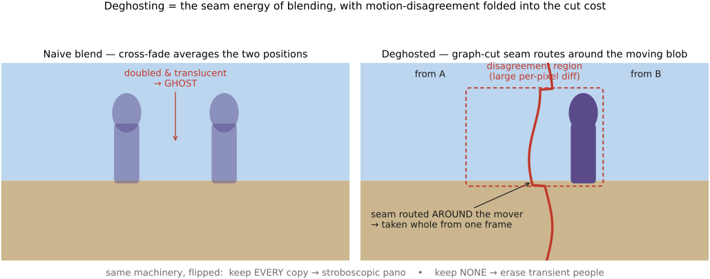
**seam energy** $E=\sum_p D_p(\ell_p)+\sum_{(p,q)}V_{pq}(\ell_p,\ell_q)$ (data + smoothness, minimized by graph cut)
20.3.7 The complete pipeline, end to end⧉
▸20.4 Bells and whistles⧉
fig-projections-three
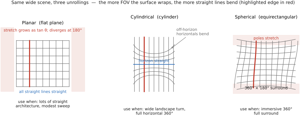
fig-projections-three · the same wide scene unrolled three ways — plane (lines straight, FOV limited), cylinder (verticals straight, full horizontal sweep), sphere (full surround, everything curves) — with a "use when" each 🟨
⬜ figure not yet created
`fig-projection-line-bending` (a straight architectural edge: planar keeps it straight but can't exceed ~120° fig-projection-line-bending
fig-bundle-drift
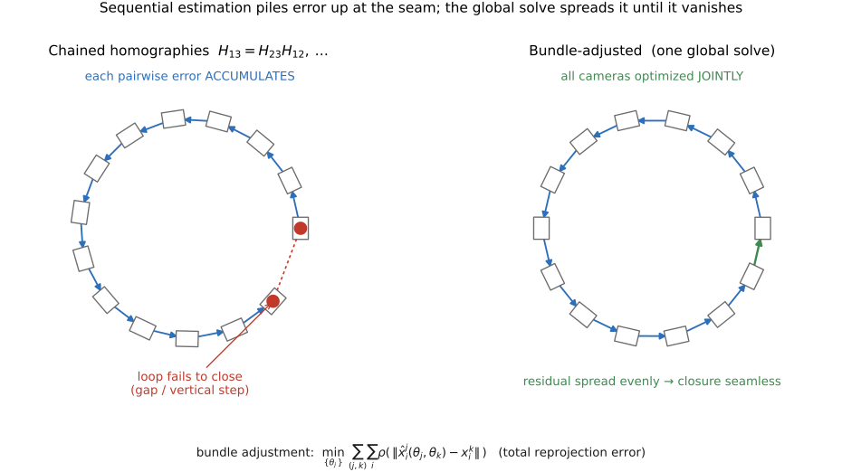
fig-bundle-drift · a chained-homography 360° panorama (visible gap from accumulated drift) vs a bundle-adjusted one (error distributed around the loop, closure seamless) 🟨
⬜ figure not yet created
`fig-gain-vignette-solve` (per-image gain + a vignetting falloff recovered jointly so overlaps agree — before/after) fig-gain-vignette-solve
fig-deghost-seam
fig-deghost-seam · a blended overlap where a walking person is doubled into a ghost vs a deghosted result that routes the seam to take the person from one frame only 🟨
fig-parallax-breaks-homography
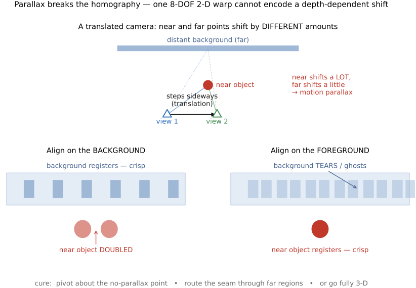
fig-parallax-breaks-homography · two shots from a translated camera where aligning the background doubles the foreground and aligning the foreground tears the background — one homography cannot handle depth-dependent parallax 🟨
The pairwise pipeline (match → RANSAC → homography → blend) makes a *demo*. A *tool* has to survive 360° loops, lens imperfections, people who wander through the shot, and a photographer who took a step sideways. Each subsection below is one such assumption breaking, and the repair. The recurring fix is the same: **treat the whole panorama as one global estimation problem instead of a chain of independent local ones.** *(To consult Ce Liu & Miki Rubinstein for the production deghosting / motion-handling and continuous-capture details — queue marker.)*
equations
**bundle adjustment** $\displaystyle \min_{\{\theta_j\}} \sum_{j,k}\sum_{i} \rho\big(\lVert \hat{\mathbf x}^j_i(\theta_j,\theta_k) - \mathbf x^k_i \rVert\big)$ — jointly over all camera params $\theta_j$ (rotation $R_j$, focal $f_j$, distortion, gain), summed over all feature correspondences $i$ across all overlapping image pairs $(j,k)$, $\rho$ a robust loss
**gain compensation** $\min_{\{g_j\}} \sum_{(j,k)}\sum_{p\in \text{overlap}} (g_j I_j(p) - g_k I_k(p))^2 + \lambda\sum_j (g_j-1)^2$
**radial distortion** $r_d = r(1+\kappa_1 r^2 + \kappa_2 r^4)$ folded into $\theta_j$
▸20.5 Continuous panoramas (e.g. on cell phones)⧉
⬜ figure not yet created
`fig-sweep-incremental` (a phone panning fig-sweep-incremental
fig-sweep-central-strip
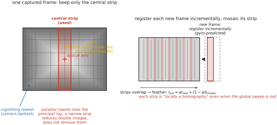
fig-sweep-central-strip · a single frame with only its central strip retained, annotated low-vignetting / low-distortion / low-parallax, and narrow overlaps feathered between strips 🟨
⬜ figure not yet created
strips overlap just enough to feather)
fig-rolling-shutter-pan
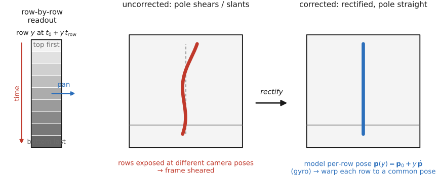
fig-rolling-shutter-pan · a slanted, sheared vertical pole from an uncorrected fast pan vs a straightened, rectified version, illustrating line-by-line CMOS readout during camera motion 🟨
fig-portrait-undistortion
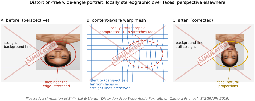
fig-portrait-undistortion · distortion-free wide-angle portraits (Shih, Lai & Liang 2019): stretched edge face → content-aware warp mesh (locally stereographic over faces, perspective elsewhere) → corrected face with straight lines preserved (Perspective distortion and its correction) ✅
A cell-phone "sweep" panorama is the same goal — one wide image from many views — but the *capture model* is inverted: instead of shooting N discrete frames and stitching offline, the phone **captures a continuous video while you pan** and builds the mosaic **as the frames arrive**. That streaming constraint, plus the fact that you're hand-holding and continuously translating, reshapes every design choice. *(To consult Ce Liu & Miki Rubinstein for the mobile-pipeline specifics — queue marker.)*
equations
**per-strip registration** incremental homography $H_{t} = H_{t-1}\,\Delta H_t$ ($\Delta H_t$ = frame-to-frame, often near pure rotation, predicted from the **gyroscope**)
**rolling-shutter** per-row pose $\mathbf p(y)=\mathbf p_0 + y\cdot \dot{\mathbf p}$ (camera moves *during* a frame's readout → row $y$ captured at time $t_0+y\,t_{\text{row}}$)
**strip feather** $I_{out}=\alpha I_{\text{new strip}} + (1-\alpha)I_{\text{mosaic}}$ across the narrow overlap