fig-results-montage
fig-demosaick-snapshot · even a plain snapshot needs computation: one colour per pixel (Bayer mosaic) → demosaicked RGB ✅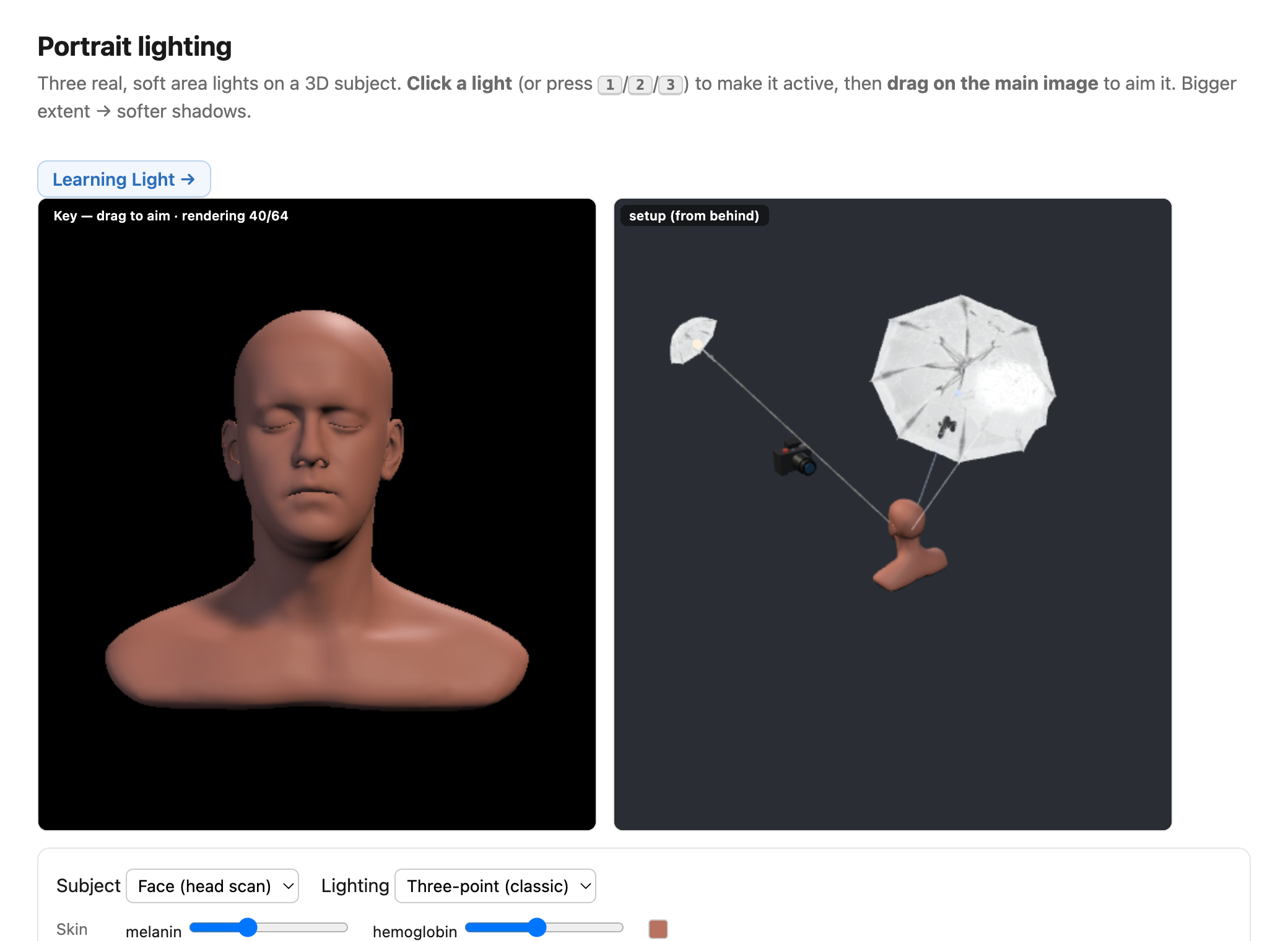
fig-portrait-lighting-sim · live portrait-lighting simulator (web edition): three soft area lights (key/fill/kicker — az/el/extent/intensity/colour, area-light-supersampled soft shadows) on a 3D face with a physiological melanin/hemoglobin skin model; a from-behind setup view with Meshy studio umbrellas + a camera rig; lighting presets; static fallback is a screenshot. *3D umbrella generated with Meshy AI.* ✅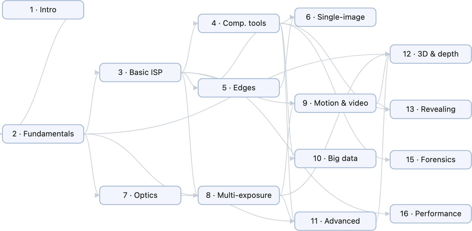
fig-chapter-dependency-graph · graph of chapter dependencies (provides/requires) so a reader can chart a path 🟨
fig-pixel-grid · a 32×32 image with each pixel a square + a zoom to the array of numbers (Image representation, INTRO) 🟨
fig-light-journey · FUNDAMENTALS part opener — the journey of light: source → scene (reflection) → lens → sensor / retina → visual system, each step labelled with its chapter ✅
fig-light-models · three models of light: wave (λ) vs ray vs particle/photon propagation, and what each is good for 🟨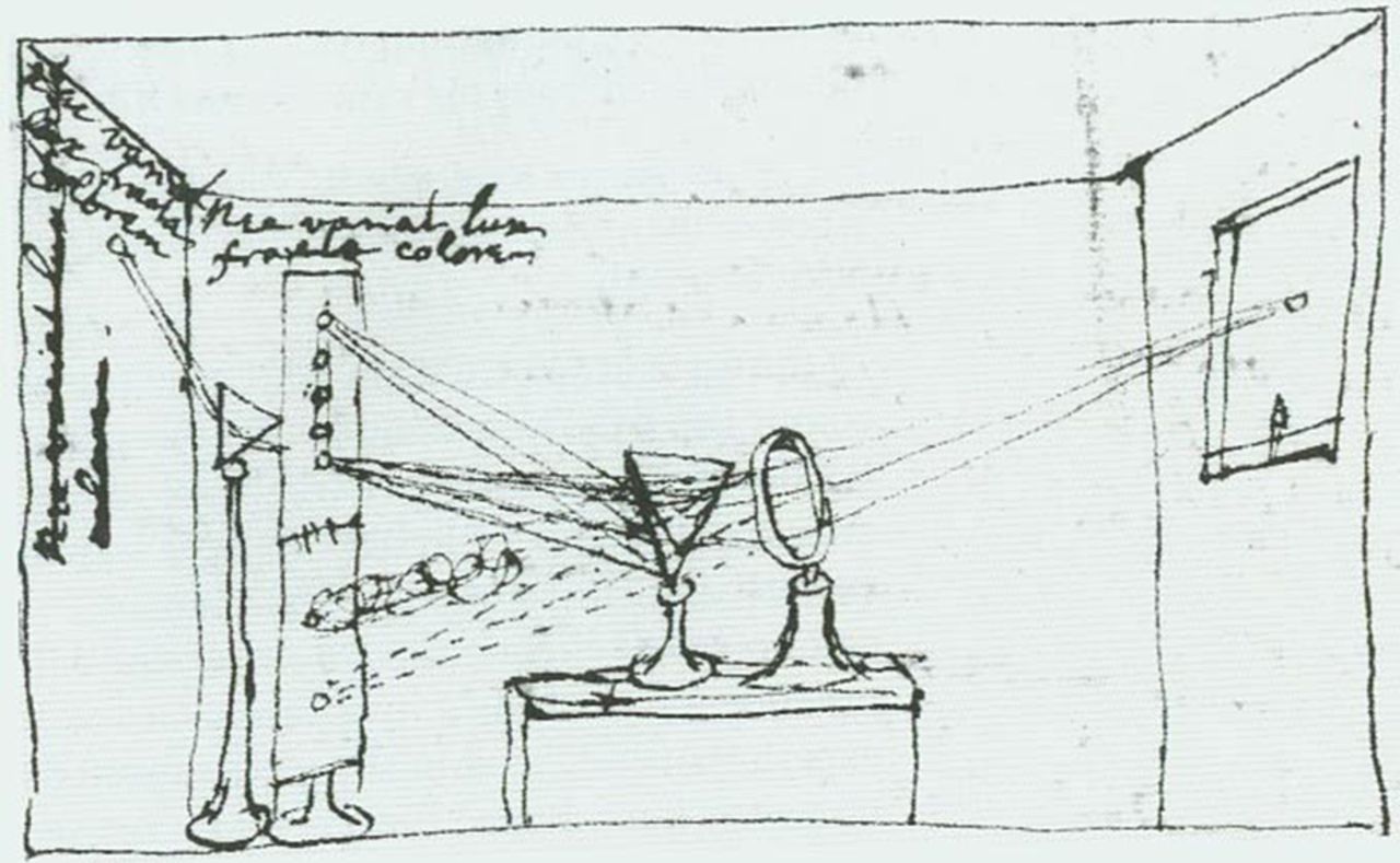
fig-newton-prism · Newton's prism experiment: white light dispersed into a spectrum (classic diagram) 🟨
fig-em-spectrum · EM spectrum / wavelength map 🟨
fig-reflection-refraction-diffraction · reflection (equal angles) · refraction (Snell, two indices) · diffraction 🟨
fig-polarization · unpolarized (random orientations) vs polarized light 🟨
fig-atmospheric-scattering · Rayleigh scattering: blue sky (short path) vs red sunset (long path) 🟨
fig-reflectance-illumination-spectra · example reflectance & illumination spectra 🟨
fig-illum-times-reflectance · light = illumination × reflectance (per-wavelength) ✅
fig-brdf · light bouncing off a surface — the BRDF (incoming/outgoing dirs, normal, reflection lobe, θ angles) 🟨
fig-diffuse-specular-spheres · Lambertian (matte) sphere vs shiny (specular) sphere — same shape/light, different BRDF 🟨
fig-global-illumination · color bleeding: a red wall casts red onto a white floor (multiple bounces) 🟨
fig-illuminant-spectra · blackbody / illuminant spectra (D65, tungsten, fluorescent) 🟨
fig-color-temperature · the (inverted) color-temperature scale: warm (low K) → cool (high K) 🟨
fig-radiance-irradiance · radiance (per direction) vs irradiance (per area) 🟨
fig-cosine-irradiance · why irradiance carries a cosine: a beam of width w vs its surface footprint L = w/cosθ 🟨
fig-seasons · sidebar — seasons: N. America in summer vs winter (sun angle → energy per area, cosine law) 🟨
fig-inverse-square-vs-radiance · point source 1/r² vs distance-invariant surface radiance 🟨
fig-diffraction-aperture-size · two apertures: a smaller one diffracts more (spread θ ≈ λ/D) 🟨
fig-airy-disk · Airy disk = diffraction-limited PSF 🟨
fig-aperture-sharpness-sweet-spot · aberration vs diffraction → sharpness sweet spot 🟨
fig-camera-obscura · camera obscura / pinhole (artist's) 🟨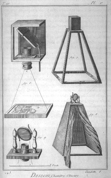
fig-camera-obscura-apparatus · camera obscura apparatus (Diderot engraving) 🟨
fig-bare-sensor-averaging · a bare sensor averages all rays 🟨
fig-pinhole-fov · pinhole geometry: real (inverted) vs virtual (upright) image plane, and focal length → field of view 🟨
fig-perspective-projection · perspective projection equation: x'=f·X/Z, y'=f·Y/Z (divide by depth, scale by f) 🟨
fig-perspective-projection-3d · perspective projection in 3D: P=(X,Y,Z) → p=(x,y) on the image plane through the pinhole 🟨
fig-perspective-vanishing-points · perspective projection + vanishing points 🟨fig-focal-length-compression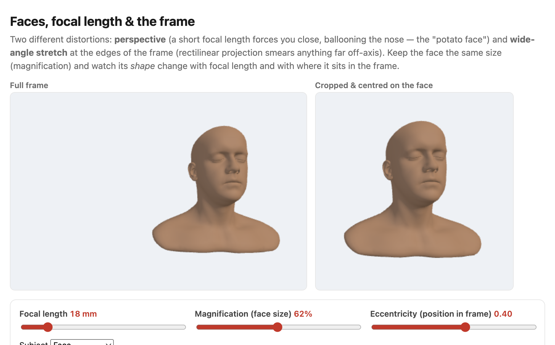
fig-face-distortion-sim · live face-distortion simulator (web edition): focal length + magnification + eccentricity controls with a full-frame view and a face-cropped view, showing the close-wide "big nose" perspective and the wide-angle edge stretch at constant face size; subject = a face, a grid sphere, or one of six diverse Meshy humans framed on the face; static fallback is a screenshot. *Human 3D models generated with Meshy AI.* ✅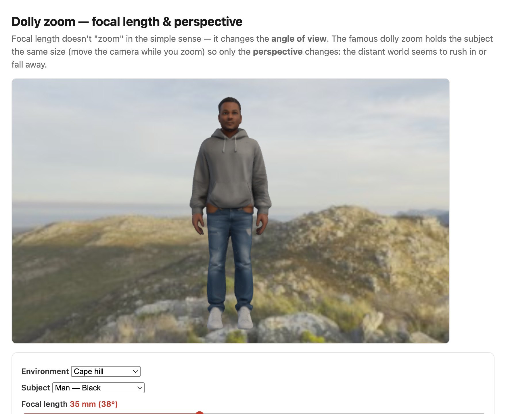
fig-dolly-zoom-sim · live dolly-zoom simulator (web edition): hold the subject size while focal length and camera distance trade off so only perspective / background scale changes; log focal (12–200 mm) + distance sliders, realistic Poly Haven environments, subject = head bust or one of six diverse Meshy humans. *Human 3D models generated with Meshy AI.* ✅fig-portrait-lighting-sim · live portrait-lighting simulator (web edition): three soft area lights (key/fill/kicker — az/el/extent/intensity/colour, area-light-supersampled soft shadows) on a 3D face with a physiological melanin/hemoglobin skin model; a from-behind setup view with Meshy studio umbrellas + a camera rig; lighting presets; static fallback is a screenshot. *3D umbrella generated with Meshy AI.* ✅
fig-keystoning-cause · keystoning is the tilt, not the lens — a camera tilted up makes world-parallel verticals converge (façade → trapezoid), while the fronto-parallel shot keeps them parallel; projection preserves lines, not parallelism 🟨
fig-point-line-duality · point↔line duality in homogeneous 2D: two points → a line, two lines → a point (same cross product) 🟨
fig-projection-decomposition · projection-matrix decomposition K·[R matplotlib, 3-stage pipeline
fig-crop-focal-length · cropping = changing focal length: full frame vs a crop box ≡ a longer-focal-length capture, upsampled 🟨
fig-depth-vs-ray-length · depth (z coordinate) vs ray length ‖P‖ from camera to a 3D point; unproject (pixel + depth → 3D) 🟨
fig-single-lens-refraction · single lens, two interfaces, Snell at each → focus 🟨
fig-thick-lens-snell · thick lens: Snell's law at both interfaces, with the incidence/refraction angles and indices of refraction shown 🟨
fig-fermat-equal-path · the Fermat / equal-optical-path view of a lens: several rays object→focus, all the same optical path (glass detour offsets the slower speed) 🟨
fig-thick-lens-wave-sim · live 2-D FDTD wave sim of a **thick biconvex lens** focusing: a point source's diverging wave is reshaped by the slower glass into a converging one that meets at an image point; focus tracks 1/f=(n−1)2/R and 1/v=1/f−1/u (Fundamentals → Lens image formation, Fermat/equal-path) ✅
fig-thin-lens-rays · thin-lens ray diagram (focus, focal point) 🟨
fig-thin-lens-conjugates · conjugates: object at ∞ / far / close / at focal length → where the image forms 🟨
fig-circle-of-confusion · finite aperture & circle of confusion ✅
fig-defocus-vs-parameters · defocus blur (CoC) vs aperture and object distance 🟨
fig-depth-of-field · near/far limits where blur reaches c (linearized DoF) 🟨
fig-dof-derivation-near · near (front) limit by similar triangles — all quantities 🟨
fig-dof-derivation-far · far (back) limit by similar triangles — all quantities 🟨
fig-dof-vs-parameters · DoF vs aperture, focal length, focus distance 🟨
fig-hyperfocal · hyperfocal: focus at H → sharp from H/2 to ∞ 🟨
fig-dof-same-framing · same framing + same f-number → same object-space DoF (short vs long focal length); background blur still looks larger with the long lens 🟨
fig-dof-double-cone · object-space DoF as a double cone in front of the lens, waist on the focus plane (the blur for one scene point) 🟨
fig-dof-depth-dependent · defocus is NOT a convolution: blur radius depends on scene depth (not pixel location), and occlusion at depth edges 🟨
fig-dof-background-blur · DoF focal-length invariance is only first-order: background blur c vs background distance for 35/85/200 mm (matched framing & N) coincide near the subject and fan apart far away; + c vs focal length showing growth/saturation ✅
fig-contrast-af-curve · contrast-detect AF: high-frequency contrast (sharpness) vs focus position, peaked at best focus; hill-climb arrows that must overshoot past the peak then step back (no direction cue) ✅
fig-pixel-measurement-integral · a pixel value = integral over aperture (thin lens ellipse) + finite pixel area (+ time, wavelength); the 4 domains → DoF, antialiasing, motion blur, color; linked to the plenoptic function 🟨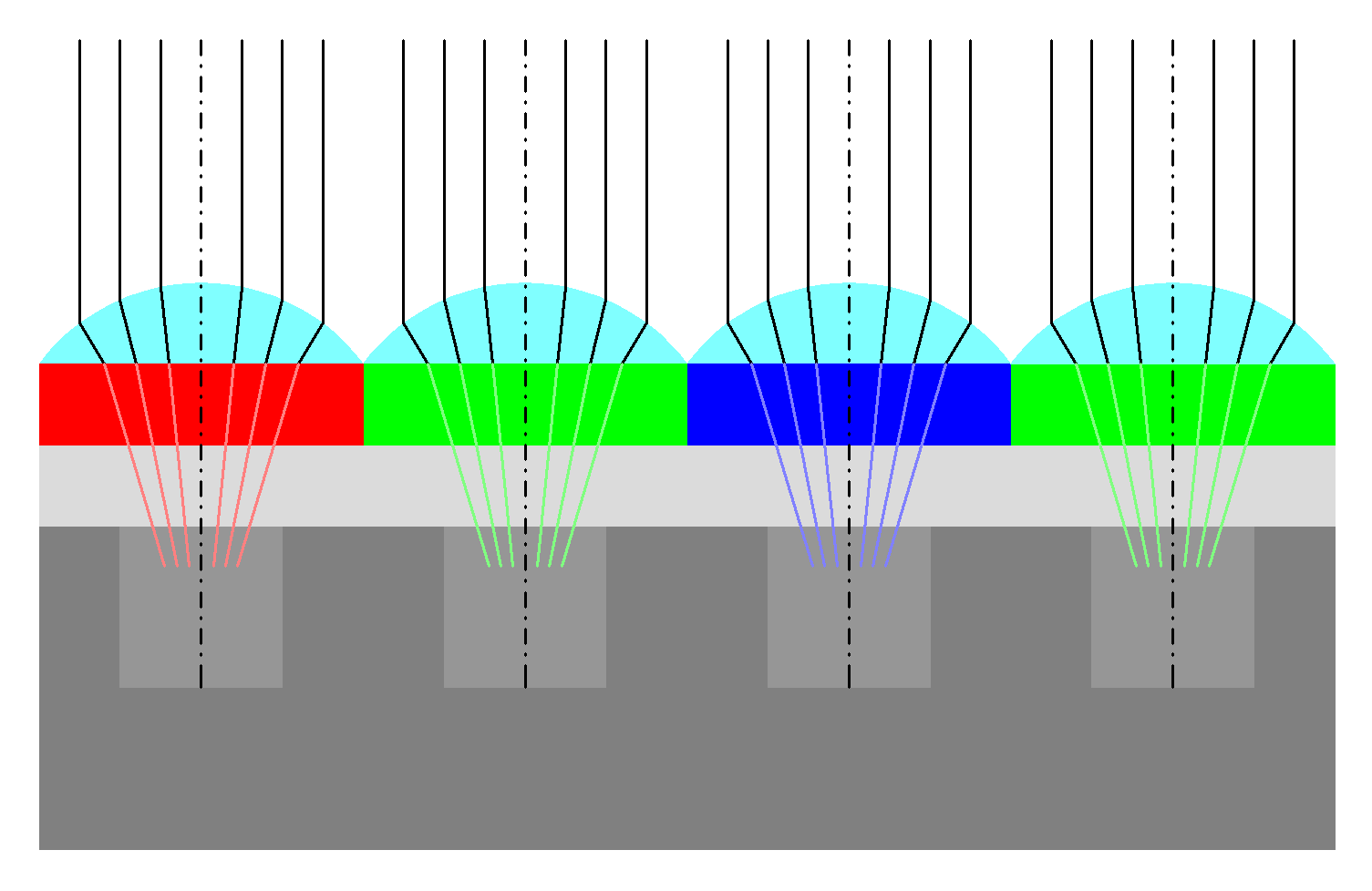
fig-sensor-microlens · sensor cross-section: microlens → filter → photosite 🟨
fig-rolling-shutter-pan · a slanted, sheared vertical pole from an uncorrected fast pan vs a straightened, rectified version, illustrating line-by-line CMOS readout during camera motion 🟨
fig-slowmo-axis · four ways to treat the time axis on a shared timeline — normal capture (sparse), high-speed (dense true samples), interpolation (sparse reals with synthesized in-betweens), and long-exposure blur (the integral); only interpolation adds resolution after capture and can be wrong 🟨
fig-mirrorless-anatomy · labeled cutaway of a mirrorless full-frame camera (lens+mount, sensor/IBIS, mech+electronic shutter, EVF, processor/on-sensor PDAF, card+battery); SLR mirror-box inset for contrast ✅
fig-rolling-shutter-skew · rolling-shutter distortion — a global shutter keeping a vertical pole upright under a fast pan vs a rolling shutter where per-row readout $t(r)=t_\text{frame}+r\,t_\text{row}$ shears the pole and smears fan blades (the jello effect) 🟨
fig-flash-sync · flash & focal-plane-shutter sync: whole frame ≤ X-sync · slit/partial frame above it · high-speed-sync pulse train; fill-flash noted ✅
fig-darkroom-dodge-burn · the darkroom ancestor: dodging (hold back light) and burning (add light) under the enlarger as hand-painted spatially-varying exposure 🟨fig-noise-histogramfig-noise-vs-iso
fig-noise-affine · measured noise variance is affine in brightness (σ²≈gain·I+read²) — real per-pixel variance vs mean from a 50-frame aligned ISO-3200 burst, with the affine fit, read-noise floor, and highlight roll-off (Noise, SNR, dynamic range) ✅
fig-noise-gaussian-pixels · a single pixel's value across many frames is ≈ Gaussian — per-pixel histograms from the ISO-3200 burst with Gaussian overlays (Noise) ✅
fig-noise-truncation · noise clips at black/white so it is not zero-mean at the extremes — a near-black pixel pinned at 0 ~44% of frames, its average biased bright, vs an unbiased midtone (Noise; denoising trap) ✅
fig-snr-vs-stddev · noise std-dev map vs SNR map of a brightness ramp: std rises with brightness (∝√N), but SNR=√N is worst in the shadows 🟨fig-underexposure-recovery-ff-vs-phonefig-results-montage
fig-dynamic-range-comparison · dynamic-range ladder in **stops** (horizontal bars): colour slide (~5–6) · reflective print (~6–7) · film negative (~12–13) · phone sensor (~10–12) · full-frame sensor (~14) · human eye instantaneous (~10–14) vs adapted (~20+) · an animal example · a typical sun-and-shadow scene (>20) — shows why no single capture holds a high-contrast scene (→ HDR) ✅fig-stereo-pair
fig-disparity-geometry · parallel-camera disparity geometry 🟨fig-disparity-map
fig-random-dot-stereogram · a random-dot stereogram pair (Julesz): a shifted central patch → depth from disparity alone, no monocular cues 🟨
fig-epipolar-line · the epipolar constraint: two views of a 3-D point, epipolar plane & line, the match constrained to a 1-D search ✅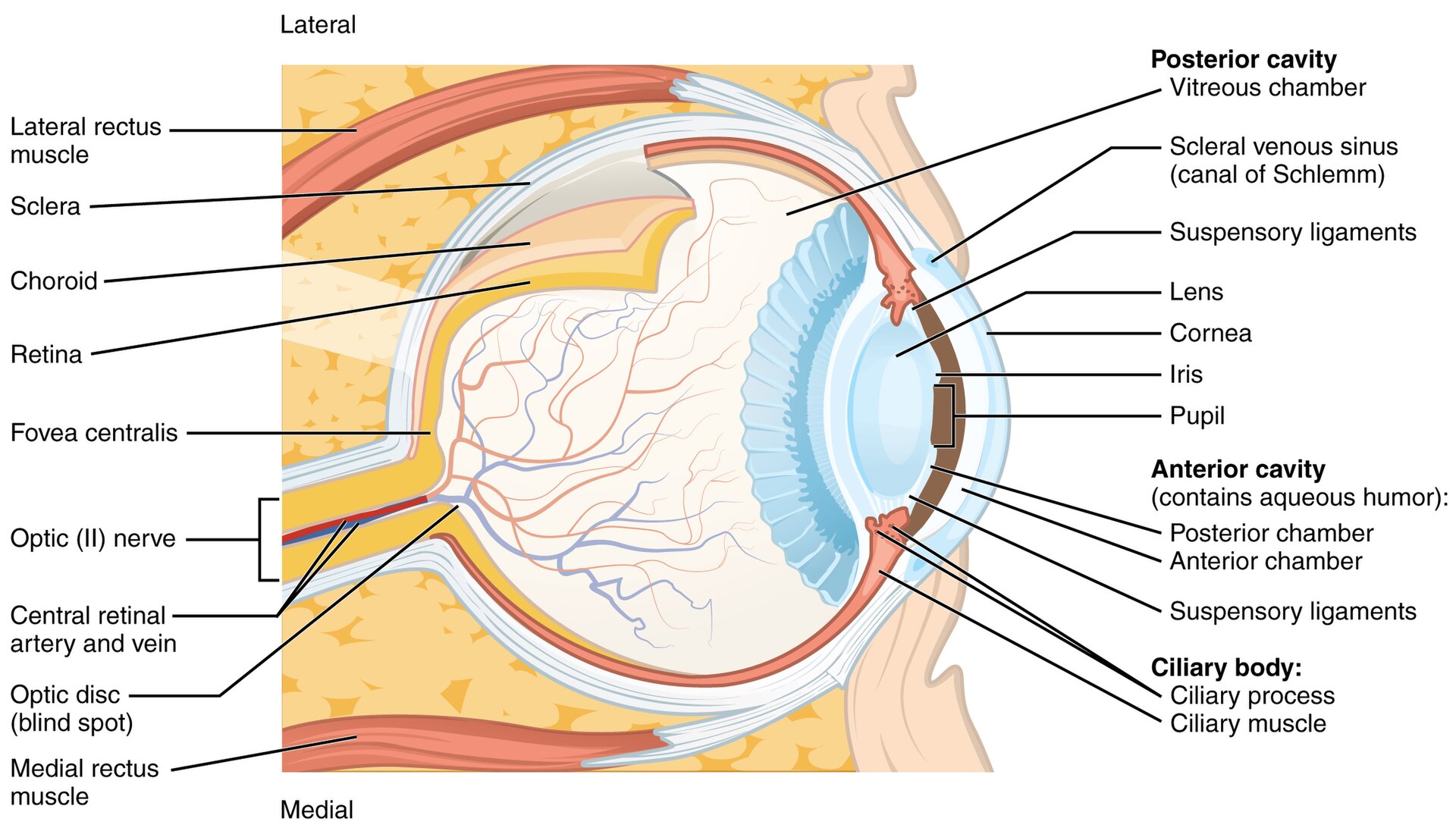
fig-eye-cross-section · eye cross-section 🟨
fig-retina-layers · retina layers & photoreceptor synapses 🟨
fig-cone-rod-distribution · cone/rod distribution & fovea 🟨
fig-visual-pathway · pathway retina→LGN→V1 🟨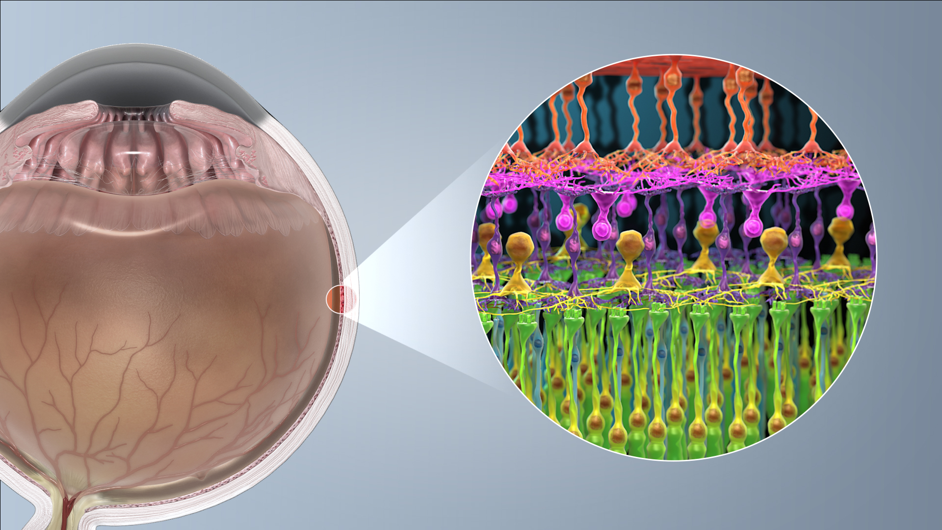
fig-photoreceptor-cell · anatomy of a rod & cone cell 🟨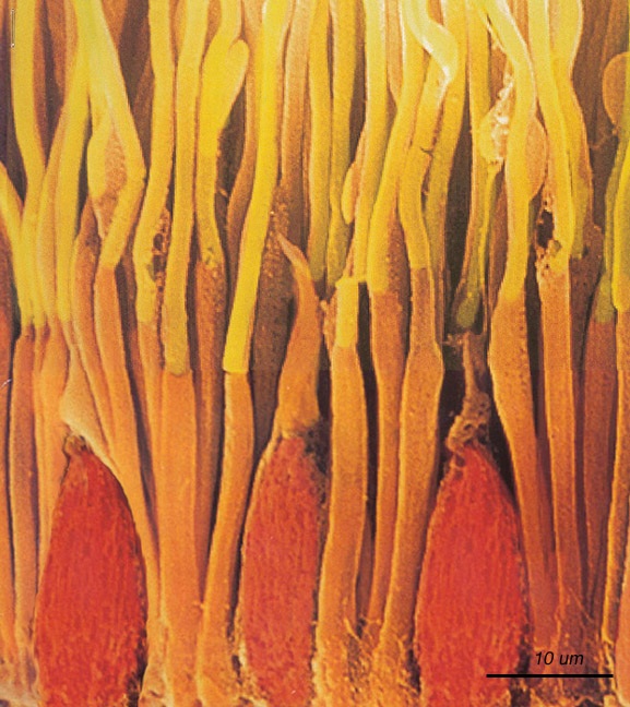
fig-rods-cones-micrograph · micrograph of rods & cones (primate retina) 🟨
fig-cone-sensitivities · cone spectral sensitivities (L/M/S) 🟨
fig-spectrum-to-three-responses · spectrum → 3 responses (projection) 🟨
fig-metamers · metamers (two spectra, one color) 🟨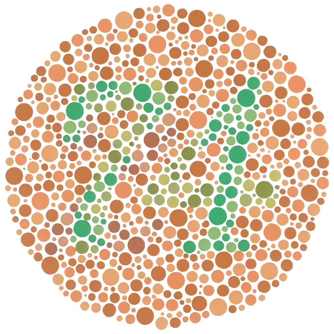
fig-ishihara · Ishihara plate (“74”) 🟨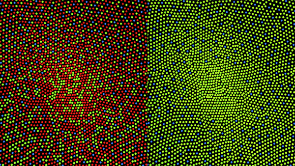
fig-cone-mosaic · trichromatic cone mosaic (L/M/S, fovea) 🟨
fig-cone-response-matrix · cone response as a 3×N matrix–vector product r = C·E (discretized λ); note the continuous / infinite-D limit r_k = ∫ c_k(λ) E(λ) dλ 🟨
fig-nonorthogonal-dual-basis · non-orthogonal cone basis (two vectors in the positive quadrant) and its dual: synthesis vs analysis; the dual (analysis) basis has negative coordinates 🟨
fig-opsin-tree · the opsin gene tree (schematic): ancestral opsin → RH1 rod + cone classes (SWS1/SWS2/RH2/LWS); the human S/M/L branch highlighted, with the recent primate L/M gene duplication marked ✅
fig-opponent-channels · opponent channels (R–G, B–Y, light–dark) 🟨
fig-afterimage · afterimage demo 🟨
fig-spanish-castle · afterimage / Spanish-Castle illusion ✅
fig-photopic-scotopic-range · the photopic / mesopic / scotopic regimes on a horizontal log-luminance axis (cd/m², ~10⁻⁶→10⁸): rod vs cone activity bands, the absolute threshold, the Purkinje shift, and landmarks (starlight, moonlight, indoor, overcast, sunlight, the sun); the eye's full range vs the few-log instantaneous range (→ adaptation, HDR) ✅
fig-checker-shadow · Adelson's checker-shadow illusion — the original artwork: the illusion (squares A/B identical luminance) beside the equal-grey-bars proof ✅
fig-white-balance-real · white balance computed from scratch (von Kries per-channel gain in linear light): a warm-casted photo corrected by gray-world vs white-patch/max-RGB, with the recovered channel gains (PS1) ✅fig-wb-before-afterfig-the-dress
fig-simultaneous-contrast · simultaneous-contrast patch 🟨
fig-mach-bands · Mach bands 🟨
fig-contrast-ratios · contrast-as-ratios strip 🟨
fig-campbell-robson · Campbell–Robson CSF chart 🟨
fig-acuity-chart · an acuity chart 🟨
fig-csf-chromatic · three contrast-sensitivity functions: luminance (band-pass) vs red–green and blue–yellow (low-pass, lower cutoff) — we resolve colour more coarsely than brightness 🟨
fig-blur-chroma-luma · blur only the chroma (Lab) and the image still looks sharp; blur the luminance and it falls apart — the basis for chroma subsampling ✅fig-scanpath
fig-hunt-effect · colorfulness vs luminance (Hunt) 🟨
fig-bezold-brucke-abney · Bezold–Brücke / Abney demos ✅
fig-eye-evolution · the evolution of the eye, in cross-sections: flat photoreceptor patch (no image) → cup (directional) → pinhole (an image, no lens) → lensed eye — recapitulating sensor → camera-obscura → lens (Bonus: animal eyes) 🟨
fig-analysis-vs-synthesis · analysis vs synthesis (sense→3 / reproduce←few) 🟨
fig-color-matching-setup · color-matching experiment setup ✅
fig-cie-cmfs · CIE color-matching functions 🟨
fig-chromaticity-diagram · xy chromaticity + spectral locus + white point 🟨
fig-gamma-curves · gamma encode/decode curves 🟨
fig-quantization-banding · quantization banding (low-bit demo), worst in shadows ✅
fig-slr-cross-section · labelled cross-section of an SLR: 45° main reflex mirror sends light UP to the focusing screen + pentaprism → optical viewfinder; the semi-transparent main mirror + secondary (sub) mirror fold light DOWN to the phase-detect AF module in the mirror-box floor; focal-plane shutter + sensor/film behind; inset shows the mirror flipping up for exposure (companion to `fig-mirrorless-anatomy`) ✅
fig-rgb-cube · RGB cube 🟨
fig-gamut-primaries · sRGB vs wide-gamut primaries on xy 🟨
fig-perceptual-uniformity · a rainbow at N colours equally spaced in sRGB vs CIELAB; ΔE bars under each strip show sRGB steps are perceptually ragged, CIELAB steps even (Color technology — CIELAB) 🟩
fig-cielab-space · CIELAB space 🟨
fig-cielab-ab-plane · the a*b* plane 🟨
fig-additive-subtractive · additive vs subtractive synthesis 🟨
fig-color-synthesis-bands · additive vs subtractive synthesis, 3-band cartoon; subtractive is multiplicative (Color technology) 🟨
fig-subtractive-spectra · subtractive mixing as a per-wavelength multiplication: yellow & cyan filter transmittances and their product T_Y·T_C (= green) 🟨
fig-gamut-mapping · gamut + gamut mapping 🟨
fig-repro-monochromatic · reproducing a monochromatic signal (2D LA analogy) 🟨
fig-icc-workflow · ICC workflow diagram 🟨
fig-device-gamut-mismatch · gamut mismatch across devices ✅
fig-color-multiplexing · four colour-sensing multiplexing strategies: temporal, spatial (Bayer), beam-split prism, depth (Foveon) 🟨fig-prokudin-gorskii
fig-point-op-saturation-vibrance · uniform saturation (constant `s`, over-saturates already-vivid colours → clip) vs vibrance (per-pixel gain `g = 1+v(1−sat)·w_skin(hue)`, protects vivid colours & skin): input, saturation, vibrance + a gain-vs-saturation panel (Point operations → Basic colour enhancement, BASIC) 🟩
fig-bw-conversions · one colour photo → black & white several ways: single channel (R/G/B) · average · weighted luminance · red-filter channel mix (dark sky) · an isoluminant pair collapsing to one grey — the choices differ (Converting to B&W, Color technology) ✅
fig-color-dimensions · the dimensions of color (hue/chroma/lightness) 🟨
fig-color-solid · a perceptual color solid ✅
fig-skin-tone-vectorscope · skin-tone locus on a vectorscope ✅fig-diverse-skin-tonesfig-shirley-card
fig-exposure-triangle · exposure triangle 🟨
fig-fstop-progression · f-stop power-of-two progression 🟨 pilot renderedfig-aperture-doffig-shutter-motion-blurfig-metering-18-gray
fig-ettr-histogram · expose-to-the-right: an image histogram pushed toward the highlights without clipping (vs an under-exposed one bunched at the noise floor) 🟨
fig-mode-dial · exposure mode dial (P/A/S/M) → who sets aperture vs shutter in the exposure triangle ✅
fig-telephoto-vs-retrofocus · two two-group schematics — telephoto (+ then −, principal plane H′ pushed in front → physical length < f) vs retrofocus/inverted-telephoto (− then +, long back-focal distance to clear the SLR mirror); marks f vs physical length, H′, F′ ✅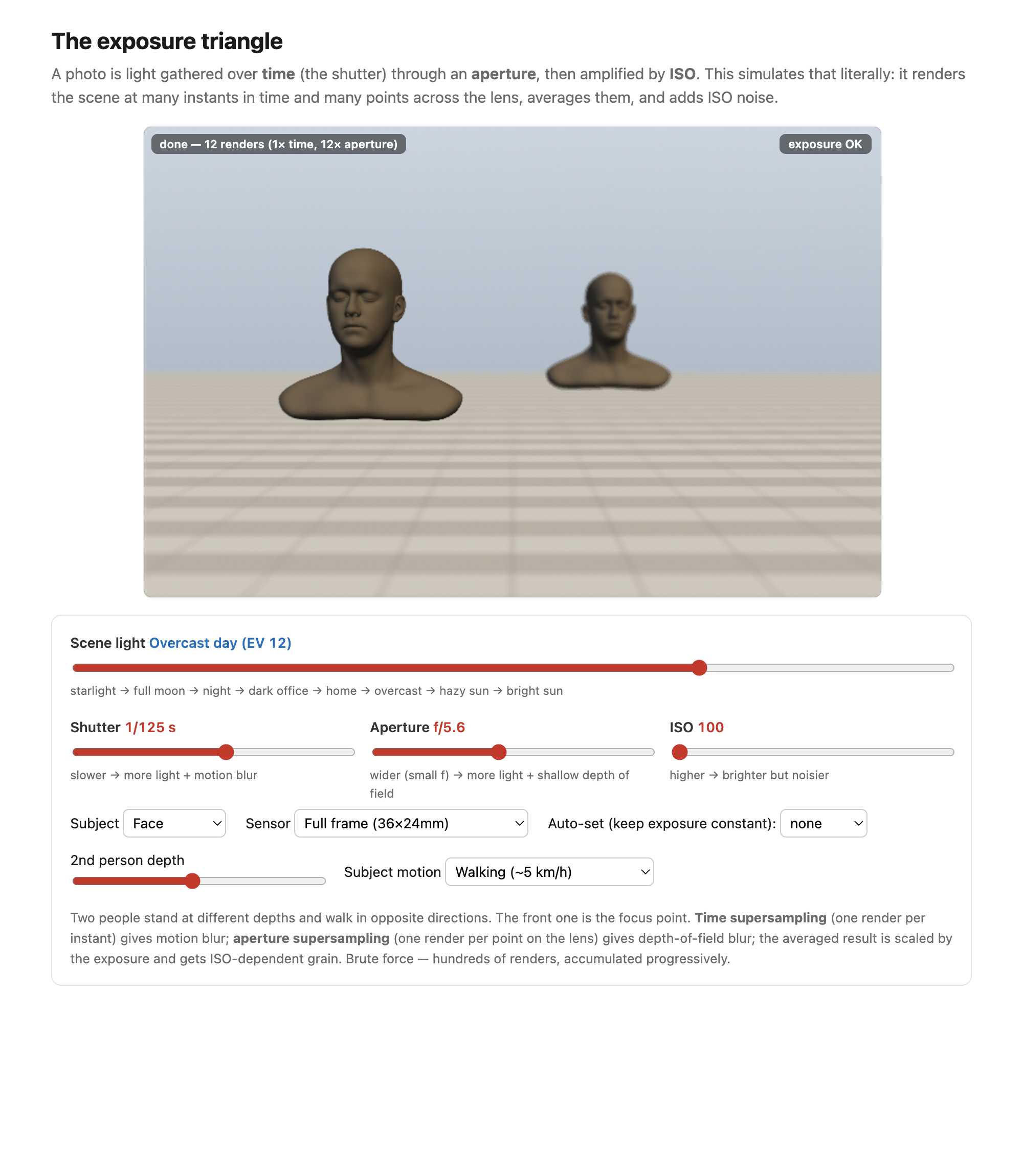
fig-exposure-triangle-sim · live exposure-triangle simulator (web edition): two 3D subjects at different depths walking opposite ways; shutter/aperture/ISO/scene-light/sensor sliders with brute-force time + aperture supersampling (real motion blur, depth of field, shot+read noise) and an auto-set triangle; static fallback is a screenshot ✅
fig-af-families · autofocus families: contrast-detect hill-climb · phase-detect sub-aperture offset · on-sensor/dual-pixel PDAF ✅fig-telephoto-vs-retrofocus · two two-group schematics — telephoto (+ then −, principal plane H′ pushed in front → physical length < f) vs retrofocus/inverted-telephoto (− then +, long back-focal distance to clear the SLR mirror); marks f vs physical length, H′, F′ ✅
fig-focus-conjugate-move · focusing geometry: as subject distance u changes the image distance v must change (1/f=1/u+1/v); the lens slides to keep the image plane on the fixed sensor — near vs far focus (lens extends vs retracts) ✅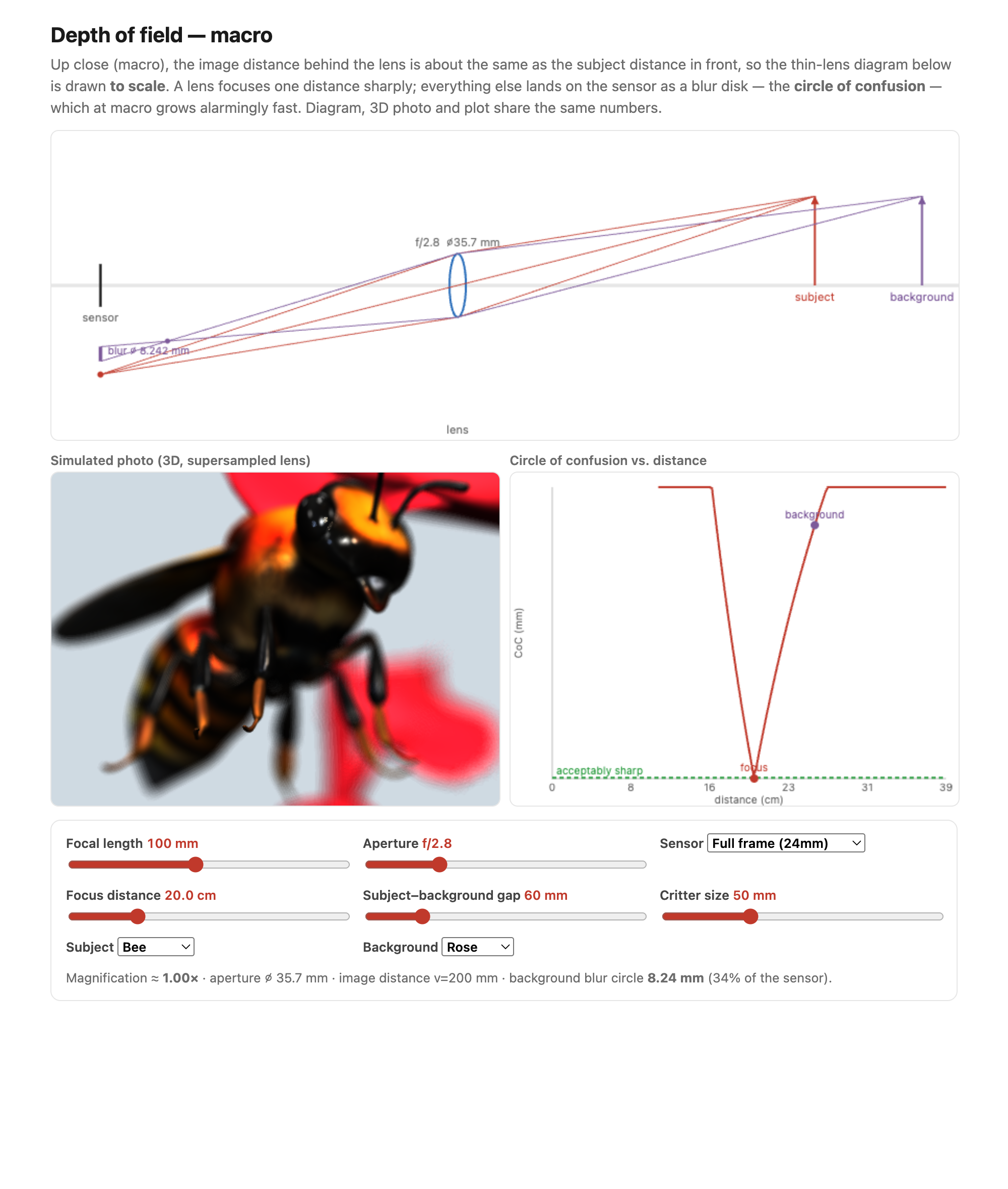
fig-depth-of-field-sim · live macro depth-of-field simulator (web edition): a to-scale thin-lens diagram + a 3D photo (aperture-supersampled bokeh) + a circle-of-confusion plot all sharing one optics model; subject dropdown (Meshy beetle / bee / ladybug) over a flower background, focus landing on the front of the face so the body and antennae blur; static fallback is a screenshot. *Bug & flower 3D models generated with Meshy AI.* ✅
fig-focal-length-families · focal-length families as nested FOV cones (ultrawide/wide/normal/short-tele/tele) with angle of view + one-word use each ✅fig-telephoto-vs-retrofocus · two two-group schematics — telephoto (+ then −, principal plane H′ pushed in front → physical length < f) vs retrofocus/inverted-telephoto (− then +, long back-focal distance to clear the SLR mirror); marks f vs physical length, H′, F′ ✅fig-dolly-zoom-sim · live dolly-zoom simulator (web edition): hold the subject size while focal length and camera distance trade off so only perspective / background scale changes; log focal (12–200 mm) + distance sliders, realistic Poly Haven environments, subject = head bust or one of six diverse Meshy humans. *Human 3D models generated with Meshy AI.* ✅
fig-reflection-removal-cues · cues that separate a window reflection from the transmitted scene — ghosting/double-image, polarization, focus difference 🟨fig-gain-vignette-solve
fig-jpeg-artifacts-photo · JPEG blocking & ringing on a REAL photographic edge (white egret vs dark foliage) at q=10: grid-aligned zoom with 8×8 overlay — blocking in the smooth area, ringing along the edge (File formats, BASIC) ✅
fig-lens-flare-ghosting · stray light: a bright source, a ray reflecting off two internal lens surfaces → a "ghost" landing displaced on the sensor, plus a veiling-glare wash; ghost vs flare labelled ✅
fig-ois-vs-ibis · two stabilization strategies side-by-side: lens-shift OIS (floating lens group moves) vs sensor-shift IBIS (sensor moves on a magnetic stage), moving element highlighted, same gyro/IMU input ✅fig-telephoto-vs-retrofocus · two two-group schematics — telephoto (+ then −, principal plane H′ pushed in front → physical length < f) vs retrofocus/inverted-telephoto (− then +, long back-focal distance to clear the SLR mirror); marks f vs physical length, H′, F′ ✅
fig-stabilization · image stabilization: hand-held blur vs OIS (lens shift) vs IBIS (sensor shift); ~2–5 stops, camera shake not subject motion ✅
fig-viewfinder-types · viewfinder types: OVF (optical) vs EVF (electronic) vs rear LCD ✅fig-telephoto-vs-retrofocus · two two-group schematics — telephoto (+ then −, principal plane H′ pushed in front → physical length < f) vs retrofocus/inverted-telephoto (− then +, long back-focal distance to clear the SLR mirror); marks f vs physical length, H′, F′ ✅fig-ettr-histogram · expose-to-the-right: an image histogram pushed toward the highlights without clipping (vs an under-exposed one bunched at the noise floor) 🟨fig-depth-of-field-sim · live macro depth-of-field simulator (web edition): a to-scale thin-lens diagram + a 3D photo (aperture-supersampled bokeh) + a circle-of-confusion plot all sharing one optics model; subject dropdown (Meshy beetle / bee / ladybug) over a flower background, focus landing on the front of the face so the body and antennae blur; static fallback is a screenshot. *Bug & flower 3D models generated with Meshy AI.* ✅
fig-shutter-angle · shutter angle sets the blur — a rotating-disc shutter at $0°/180°/360°$ admitting a smaller/larger fraction of the frame interval $T$; $180°$ ($\tau=T/2$) is the cinematic film-look, small angles strobe 🟨fig-rolling-shutter-skew · rolling-shutter distortion — a global shutter keeping a vertical pole upright under a fast pan vs a rolling shutter where per-row readout $t(r)=t_\text{frame}+r\,t_\text{row}$ shears the pole and smears fan blades (the jello effect) 🟨
fig-bokeh-shapes · bokeh: out-of-focus highlights take the aperture's shape — circular (many blades / wide open) vs polygonal (few blades, stopped down); synthetic defocus-disk fields + aperture insets ✅fig-mirrorless-anatomy · labeled cutaway of a mirrorless full-frame camera (lens+mount, sensor/IBIS, mech+electronic shutter, EVF, processor/on-sensor PDAF, card+battery); SLR mirror-box inset for contrast ✅fig-telephoto-vs-retrofocus · two two-group schematics — telephoto (+ then −, principal plane H′ pushed in front → physical length < f) vs retrofocus/inverted-telephoto (− then +, long back-focal distance to clear the SLR mirror); marks f vs physical length, H′, F′ ✅
fig-phone-camera-array · phone multi-camera array (ultrawide/wide/tele+periscope, tiny sensors, bright fixed lenses) → a computational-pipeline block → final photo ✅fig-telephoto-vs-retrofocus · two two-group schematics — telephoto (+ then −, principal plane H′ pushed in front → physical length < f) vs retrofocus/inverted-telephoto (− then +, long back-focal distance to clear the SLR mirror); marks f vs physical length, H′, F′ ✅fig-newton-prism · Newton's prism experiment: white light dispersed into a spectrum (classic diagram) 🟨fig-dynamic-range-comparison · dynamic-range ladder in **stops** (horizontal bars): colour slide (~5–6) · reflective print (~6–7) · film negative (~12–13) · phone sensor (~10–12) · full-frame sensor (~14) · human eye instantaneous (~10–14) vs adapted (~20+) · an animal example · a typical sun-and-shadow scene (>20) — shows why no single capture holds a high-contrast scene (→ HDR) ✅
fig-lens-design-tradeoff · lens-design Pareto cartoon as a 6-axis radar (sharpness, speed, size, weight, cost, distortion): fast pro prime vs compact phone lens overlaid, plus a dashed polygon showing where software correction shifts the phone lens (Lens optimization) ✅
fig-lagrangian-vs-eulerian · the organizing diagram — Lagrangian (arrows following particles over time → flow and tracking, output trajectories) vs Eulerian (a fixed grid, each pixel plotting intensity-over-time → magnification, never asking where anything went) 🟨
fig-pinhole-imaging · imaging-scenario series (2/3): add a pinhole to the bare sensor — one ray per scene point → a dim **inverted** image (same tree+sensor+colours as fig-bare-sensor-averaging) ✅fig-telephoto-vs-retrofocus · two two-group schematics — telephoto (+ then −, principal plane H′ pushed in front → physical length < f) vs retrofocus/inverted-telephoto (− then +, long back-focal distance to clear the SLR mirror); marks f vs physical length, H′, F′ ✅
fig-point-op-levels · levels on a real (flat/hazy) photo: bunched-up luma histogram stretched out to fill [0,1] by setting a black point and a white point — input + after + transfer curve with the clip-and-stretch anchors and the two histograms (Point operations → Black point, white point, and levels, BASIC) ✅
fig-wide-angle-perspective-distortion · wide-angle perspective distortion: off-axis spheres image as radially-stretched ellipses (flat-sensor geometry), and faces near a wide frame's edge are widened — not a lens flaw; forward-ref to correction (Pinhole image formation) ✅fig-flash-sync · flash & focal-plane-shutter sync: whole frame ≤ X-sync · slit/partial frame above it · high-speed-sync pulse train; fill-flash noted ✅fig-telephoto-vs-retrofocus · two two-group schematics — telephoto (+ then −, principal plane H′ pushed in front → physical length < f) vs retrofocus/inverted-telephoto (− then +, long back-focal distance to clear the SLR mirror); marks f vs physical length, H′, F′ ✅fig-darkroom-enlargerfig-telephoto-vs-retrofocus · two two-group schematics — telephoto (+ then −, principal plane H′ pushed in front → physical length < f) vs retrofocus/inverted-telephoto (− then +, long back-focal distance to clear the SLR mirror); marks f vs physical length, H′, F′ ✅fig-editing-lr-vs-ps
fig-image-memory-layout · a 2×3 RGB image packed into 1-D memory two ways — interleaved HWC (NumPy) vs planar CHW (ML), with the stride formulas (Image representation, BASIC) 🟨
fig-edge-handling-photo · the four edge modes on a real crop — black / clamp / mirror / wrap continued past the border; real-image companion to `fig-edge-handling` (Image representation → falling off the edge, BASIC) ✅
fig-operation-types · the three image-operation types — range (point) vs domain (spatial) vs neighborhood (Values / point ops, BASIC) 🟨
fig-point-op-exposure · exposure as a multiply in linear light: input, output (+1 stop), and the remapping curve (Basic Image Processing → point operations) 🟨
fig-point-op-exposure-spaces · exposure +1 stop done right (linear light) vs naively on the gamma values (over-brightens, clips at input ½): two outputs + remapping curves 🟨
fig-point-op-brightness-vs-exposure · brightness (additive, lifts blacks → milky) vs exposure (×2 in linear light, keeps 0→0): two outputs + both remapping curves 🟨
fig-point-op-contrast · contrast as a steeper tone curve about a mid-gray pivot: input, output, and the remapping curve (Basic Image Processing → point operations) 🟨
fig-point-op-contrast-spaces · the same contrast (×gain about mid-gray) in gamma (sRGB) / linear (no gamma) / log: three outputs + remapping curves (linear crushes shadows, log preserves them; black clamped to ε for log) 🟨fig-point-op-saturation-vibrance · uniform saturation (constant `s`, over-saturates already-vivid colours → clip) vs vibrance (per-pixel gain `g = 1+v(1−sat)·w_skin(hue)`, protects vivid colours & skin): input, saturation, vibrance + a gain-vs-saturation panel (Point operations → Basic colour enhancement, BASIC) 🟩
fig-histogram · an image histogram (per-channel) + cumulative histogram; its shape depends on the encoding space (BASIC tone mapping) 🟨
fig-histogram-encoding-spaces · the same image's luminance histogram in linear / gamma (sRGB) / log; 18% gray marked at 0.18 / ~0.46 / ~0.75 — the encoding reshapes the value axis (BASIC histograms) 🟩
fig-histogram-equalization · histogram equalization — the CDF used as the transfer curve, before/after (BASIC) 🟨
fig-histogram-matching · histogram matching — source + target images and their histograms → matched result, with the composed transfer curve $\text{CDF}_\text{tgt}^{-1}\circ\text{CDF}_\text{src}$ (BASIC histograms) ✅
fig-reinhard-curve · the Reinhard global tone curve L/(1+L) mapping [0,∞)→[0,1); naive clip vs Reinhard on a simulated-HDR image (BASIC) 🟨
fig-tonemap-real · global vs local tone mapping RESULT on a real HDR photo (seal at marina): naive single exposure · global Reinhard (one slope flattens local contrast → hazy) · local bilateral base+detail split (range fits, detail stays crisp) — real-image companion to `fig-tonemap-global-vs-local` (BASIC tone mapping) ✅
fig-zone-system · the Zone System strip 0–X, Zone V = 18% mid-grey (scene → print) (BASIC) 🟨
fig-convolution-slide · a kernel sliding over an image, weighted-summing a neighborhood into one output pixel (Convolution, BASIC) 🟨
fig-convolution-flip · the flip: where-from vs where-to — convolution `g(x−x')` vs correlation 🟨
fig-psf-impulse · impulse in → kernel out: convolving a Dirac reads off the PSF / impulse response 🟨
fig-blur-zoo · box vs Gaussian kernels — profiles + 2-D stencils, Gaussian truncated at ~3σ 🟨
fig-unsharp-mask · unsharp-mask decomposition: input − blur = detail (high-pass), output = input + k·detail 🟨
fig-sharpen-kernel · the sharpening kernel δ − blur as a +centre / −surround stencil 🟨
fig-separable · separability — a 2-D Gaussian = 1-D ⊗ 1-D (blur rows then columns); O(r²) → O(2r) 🟨
fig-gradient-sobel · Sobel x / y → gradient magnitude (edge strength) on an image 🟨
fig-convolution-probability · convolution as the sum of random variables: box ⊛ box = triangle (two dice) 🟨
fig-bilateral-1d · noisy step edge: noisy input vs Gaussian (smears step) vs bilateral (denoises plateaus, keeps step); side panel — per-pixel spatial×range weight collapses to one side at the edge (Bilateral filtering) ✅
fig-fourier-basis-matrix · the DFT as a change-of-basis matrix (real & imaginary parts) 🟨
fig-sine-eigenvectors · sine waves are the eigenvectors of convolution: same wave out, only amplitude/phase change 🟨
fig-fourier-2pixel · the 2-pixel example: convolution [0.8,0.2] diagonalized by a 45° rotation to [1,1]/[1,−1] 🟨
fig-fourier-magnitude-phase · an image's Fourier magnitude & phase, and the phase-swap demo (phase carries structure) 🟨
fig-compact-space-frequency · compact in space ⇔ spread in frequency (narrow vs wide Gaussian and its transform) 🟨
fig-aliasing · sampling a sine too coarsely → aliasing (high frequency folds to a low one) 🟨
fig-sampling-comb · sampling = multiply by a comb → spectral replicas; pre-filter (low-pass) before downsampling 🟨
fig-sinc-vs-practical · ideal sinc reconstruction vs a practical filter, in space and frequency 🟨
fig-deblur-preview · the deblur preview: sharp → blurred + noise → naive inverse amplifies noise; MTF 🟨
fig-svd-geometry · SVD = rotate·scale·rotate: unit circle → ellipse with semi-axes σ₁u₁, σ₂u₂ (Linear algebra) 🟩
fig-focus-stacking · optics-chapter illustrative figure (07-07 Figure 4): a stepped-focus stack → sharpness selection → all-in-focus composite. Synthetic per-slice defocus on one photo (`sourced/corn-cobs.jpg`, © Frédo Durand) — license-safe. The full real-data treatment lives in part-08 `fig-focalstack-*` ✅
fig-pixel-timeseries-bandpass · one fixed pixel, signal to output — its value over time, its temporal spectrum (a small in-band peak among DC and noise), a band-pass keeping that band, and the band scaled by $\alpha$ and added back; identical at every pixel 🟨
fig-resample-forward-inverse · concrete 2× upsampling on a 5×5 → 10×10 rainbow grid: FORWARD pushes input (i,j)→output (2i,2j) so 1 of every 2×2 output block is filled and 3 are black holes (regular lattice of gaps); INVERSE loops output, samples input via f⁻¹ (nearest) → every pixel filled (2×2 colour blocks). Forward leaves holes, inverse fills everything (Resampling, BASIC) ✅
fig-linear-interp-1d · 1-D linear interpolation — `im[1.3]` from its two neighbours 🟨
fig-bilinear · bilinear interpolation — the 4-neighbour weighting on the unit square 🟨
fig-resample-kernels-real · the kernel ladder on a REAL photo (Boston skyline + rainbow) resampled under a 35° rotation, magnified on a detail: nearest (blocky) → bilinear (smeared) → bicubic (edges restored) → Lanczos (sharpest) — adds Lanczos + the rotation case to `fig-interp-comparison` ✅
fig-reconstruction-pipeline · the resampling pipeline: sample → reconstruct → prefilter → resample 🟨
fig-aliasing-photo · aliasing/moiré on a real photo: a window-grid facade decimated with no prefilter folds into moiré bands — the 2-D, real-image companion to `fig-aliasing` (Sampling and aliasing) ✅
fig-gaussian-pyramid · the Gaussian pyramid — repeated blur + downsample tower (Pyramids, BASIC) 🟨
fig-laplacian-pyramid · the Laplacian pyramid — band-pass levels (G_k − expand(G_{k+1})) 🟨
fig-pyramid-encode-decode · the Laplacian pyramid as an encoder → decoder (exact reconstruction) 🟨
fig-pyramid-frequency-bands · each pyramid level = a frequency band (concentric Fourier rings) 🟨
fig-pyramid-blending · pyramid blending walkthrough on Earth+Jupiter — source A · source B · naive (hard mask, visible seam) · pyramid blend (seamless) ✅
fig-coring · coring — zero the small detail coefficients (noise), keep the large ones 🟨
fig-ssim-vs-mse · same PSNR, very different SSIM — pixel error ≠ perceived quality (Image metrics, BASIC) 🟨
fig-denoising-before-after · denoising a real colour crop (realistic shot+read noise): noisy vs Gaussian (smears edges) vs bilateral (edge-preserving) (Denoising, BASIC) ✅
fig-averaging-convergence · averaging N noisy frames → noise drops as 1/√N (1, 3, 9, 25 frames), on a real colour photo with realistic shot+read noise (Denoising, BASIC) ✅
fig-demosaick-real-bayer · the PS3 raw mosaic (NO-PARKING sign) demosaicked: ground truth · simulated RGGB Bayer mosaic · naive bilinear (false colour on the window grid) · green-based (clean), with a zoom (Demosaicking, BASIC) ✅
fig-demosaick-before-after · Bayer → RGB: the mosaic, naive bilinear demosaick (zipper / fringing), edge-aware (Demosaicking, BASIC) 🟨
fig-coma · coma: an off-axis parallel bundle where each annular aperture zone images to a different height; chief ray through the lens centre + zonal rays missing a common focus → the one-sided comet ("coma") spot with a head and a radial tail ✅fig-white-balance-real · white balance computed from scratch (von Kries per-channel gain in linear light): a warm-casted photo corrected by gray-world vs white-patch/max-RGB, with the recovered channel gains (PS1) ✅fig-wb-before-after
fig-von-kries · Von Kries per-channel gains 🟨fig-illuminant-metamerism
fig-isp-walk-real · the ISP pipeline walked on ONE real photo (boatman gathering lotus, overcast lake, Sony DNG): raw (linear, no WB — flat & green) · white balance · tone+colour (gamma encode) · denoise · sharpen · finished JPEG, frame-coloured by linear-light vs encoded regime — real-image companion to `fig-isp-block-diagram` (Recap ISP, BASIC) ✅fig-awb-greyworldfig-awb-mixed-failfig-light-models · three models of light: wave (λ) vs ray vs particle/photon propagation, and what each is good for 🟨fig-mixed-illuminant-scene
fig-jpeg-pipeline · the JPEG encoder — RGB → opponent colour → chroma subsample → 8×8 DCT → quantize → entropy code (File formats, BASIC) 🟨
fig-dct-basis · the 8×8 DCT-II cosine basis (DC top-left → high frequency bottom-right) 🟨
fig-chroma-subsampling · chroma subsampling grids 4:4:4 / 4:2:2 / 4:2:0 (chroma sampled coarser than luma) 🟨
fig-jpeg-artifacts · JPEG blocking & ringing at low quality (original vs q=8, zoomed crop) 🟨
fig-jpeg-quality-levels · JPEG quality sweep (q=85→40→20→10→5): the same photo's edge-crop at each quality with the whole-image file size beneath — degradation grows as size drops (File formats, BASIC) 🟩
fig-isp-block-diagram · the ISP pipeline: RAW → black level → demosaick → white balance → denoise → tone/colour → sharpen → gamma → JPEG (Recap ISP, BASIC) 🟨
fig-correspondence-then-transport · the L17 spine — one scene displaced (two views / two faces / two frames / one long frame), each resolved by estimating a coordinate map (homography, morph field, flow, track, motion vector, camera path) then transporting pixels by one shared inverse-warp engine; the finding is hard, the moving is plumbing 🟨
fig-image-as-vector · an image *is* a vector: a 5×5 pixel grid unrolled into a tall column vector; n = H·W (Linear algebra) 🟩
fig-least-squares · line fit minimizing squared vertical residuals (Optimization & regression) 🟩fig-deblur-preview · the deblur preview: sharp → blurred + noise → naive inverse amplifies noise; MTF 🟨
fig-gradient-descent · descent path on a convex-bowl contour (−∇f steps); too-large step overshoots (Optimization) 🟩
fig-pyramid-reconstruction · RECONSTRUCTION on a real photo: collapse the Laplacian pyramid coarse→fine (residual → +L_k each octave → exact image), plus an all-black per-pixel error panel (max ~1e-16 = lossless) (Reconstruction, BASIC) ✅fig-focus-stacking · optics-chapter illustrative figure (07-07 Figure 4): a stepped-focus stack → sharpness selection → all-in-focus composite. Synthetic per-slice defocus on one photo (`sourced/corn-cobs.jpg`, © Frédo Durand) — license-safe. The full real-data treatment lives in part-08 `fig-focalstack-*` ✅fig-gradient-descent · descent path on a convex-bowl contour (−∇f steps); too-large step overshoots (Optimization) 🟩fig-pyramid-reconstruction · RECONSTRUCTION on a real photo: collapse the Laplacian pyramid coarse→fine (residual → +L_k each octave → exact image), plus an all-black per-pixel error panel (max ~1e-16 = lossless) (Reconstruction, BASIC) ✅fig-focus-stacking · optics-chapter illustrative figure (07-07 Figure 4): a stepped-focus stack → sharpness selection → all-in-focus composite. Synthetic per-slice defocus on one photo (`sourced/corn-cobs.jpg`, © Frédo Durand) — license-safe. The full real-data treatment lives in part-08 `fig-focalstack-*` ✅
fig-learned-vs-handdesigned · same inverse-problem skeleton, prior swapped: classical (data-fit + hand prior $\Phi$) vs learned ($f_\theta$ fit to data) (ML) ✅
fig-synthetic-data-pipeline · manufacture (degraded, clean) training pairs by simulating the camera/degradation (ML) ✅
fig-downsample-aliasing · 3 panels: the full **high-res input** zone plate (cos r², rings finer toward the edge — what's being shrunk) → ÷4 naive decimation (drop samples) → moiré aliasing → ÷4 prefilter-then-decimate (Gaussian low-pass first) → clean ✅
fig-colorization-classical-vs-learned · Levin 2004 scribble-propagation vs Zhang 2016 fully-automatic colorization (ML) ✅fig-depth-anything
fig-gan-pix2pix · paired image-to-image translation: edge map → photo (conditional GAN) (ML) ✅
fig-metric-degradation-gallery · one clean photo vs four degradations (1-px shift, low-q JPEG, noise, blur), each labelled with PSNR + SSIM — PSNR and SSIM mostly agree but disagree where L2 is blind (shift scores worst PSNR yet looks identical; blur keeps high PSNR yet softens texture) (Image metrics, BASIC) ✅
fig-genai-evaluate-vs-sample · the generative leap (L11): a prior you can only *evaluate* ($\Phi$/denoiser) vs one you can *sample* ($x\sim p(x)$) (GenAI) ✅
fig-diffusion-forward-reverse · the two chains: forward $q$ adds Gaussian noise to a real photo; reverse $p_\theta$ denoises back (GenAI) ✅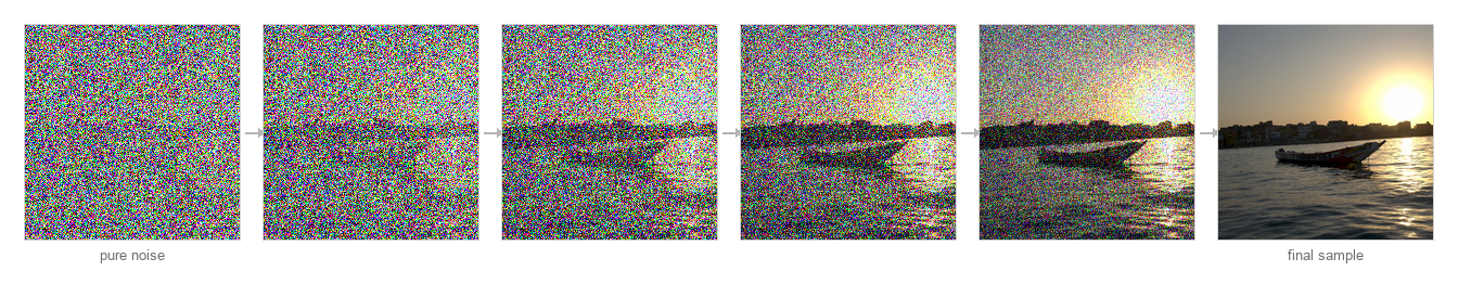
fig-diffusion-demo · live interactive demo (web edition): type a prompt and watch the reverse process denoise from noise, step by step; static fallback is a noise→photo filmstrip (GenAI) ✅
fig-denoiser-as-prior-spectrum · one PnP/RED prior slot, ever-stronger denoisers: hand-built → classical → learned → diffusion score (GenAI / Super-res) ✅
fig-latent-diffusion · encode → diffuse in a compressed latent → decode; prompt conditions by cross-attention (Stable Diffusion) (GenAI) ✅
fig-posterior-sampling · generative priors for inverse problems: one degraded $y$ → many plausible samples $x\sim p(x\mid y)$ (GenAI) ✅
fig-conditioning-controlnet · one prompt + a spatial hint (edges / pose / depth) → a generated image obeying both (GenAI) ✅
fig-seamless-cloning · Poisson seamless cloning (Pérez 2003), EDGES MATTER → Poisson editing: a disk of Jupiter cloned onto Earth — destination (target ring) · source patch · naive paste (visible ring) · Poisson paste (seam gone) ✅
fig-gradient-domain-pipeline · gradient-domain (Poisson) workflow: image → take gradients (∇f) → modify the field → integrate by solving ∇²f=div v → reconstructed (EDGES MATTER → Poisson editing) ✅
fig-mixing-gradients · mixing gradients — keep the per-pixel *stronger* gradient so destination texture shows through holey / transparent inserts (naive vs max-gradient paste) (Poisson editing) ✅
fig-poisson-vs-laplacian-blend · Poisson vs Laplacian-pyramid blending, contrasted on the DC: 1-D three cases (matched level — both agree; mismatched pedestal — Poisson re-lights, pyramid leaves a halo; constant — Poisson ramps/dissolves, pyramid keeps a feathered plateau) + 2-D (paste a constant square — Poisson dissolves it via the harmonic membrane, pyramid keeps a feathered version) ✅
fig-fourier-lowpass-highpass · low-pass vs high-pass a real photo by masking its spectrum and inverse-transforming: keep center → blurred, drop center → edges only (convolution = mult in frequency, by hand) (Reading an image's Fourier transform) ✅
fig-local-laplacian · local Laplacian filters on a real HDR sunset (Paris–Hasinoff–Kautz 2011, implemented from scratch): naive global (blown) vs Gaussian base (halo) vs local Laplacian (halo-free) tone mapping, plus the compressive remapping curve $r_g(\cdot)$ (detail centre + identity tails) and a zoom comparison proving the silhouette stays halo-free (Local Laplacian filters) ✅fig-wb-before-afterfig-pinhole-imaging · imaging-scenario series (2/3): add a pinhole to the bare sensor — one ray per scene point → a dim **inverted** image (same tree+sensor+colours as fig-bare-sensor-averaging) ✅
fig-warp-domain-vs-range · one image, two orthogonal arrows — the domain arrow bends the grid (a pixel slides, carrying its colour; a warp), the range arrow recolours in place (a point/tone op); warping moves where, not what 🟨fig-forward-warp-holes
fig-inverse-warp-lookup · inverse (output-driven) warping, the useful idiom — loop over output pixels, push each back through $f^{-1}$, sample there; every output covered once, the only difficulty a clean resampling 🟨
fig-recon-filters-1d · nearest (boxy staircase), linear (kinked through every sample), and cubic (smooth with mild overshoot) reconstruction of the same 1-D sample row — the sharpness/smoothness trade 🟨fig-bilinear-weights
fig-minify-aliasing-moire · the L16 picture — a fine grating decimated naively (folds into false moiré) vs area-averaged first then decimated (clean); same size, opposite outcomes, decided by prefiltering 🟨fig-kernel-scaling-minify
fig-dof-ladder · the degrees-of-freedom ladder — a unit square under translation (2) → similarity (4) → affine (6) → projective (8) → free-form ($\infty$), each rung breaking a preserved property 🟨
fig-mesh-triangulation-warp · piecewise-affine mesh warp — control matches triangulated, each triangle carrying its own affine map; exact and fast but only $C^0$, creasing along shared edges 🟨fig-tps-rbf-warp
fig-beier-neely-segments · Beier–Neely feature-line warp — before/after directed segments, one segment's $(u,v)$ frame, and the distance-weighted blend of several segments' proposed displacements ($w_i=(\ell_i^p/(a+d_i))^b$) 🟨
fig-arap-vs-affine · drag one handle — an unconstrained affine/least-squares warp shears and stretches, vs an as-rigid-as-possible / MLS warp that keeps each neighbourhood near a rotation so the shape bends without stretching 🟨
fig-morph-crossfade-ghost · why a cross-dissolve ghosts — two misaligned faces averaged at $t=0.5$ superimpose features into a translucent four-eyed, two-mouthed ghost; the blend handled colour but ignored position ✅
fig-morph-shape-vs-color · the two orthogonal knobs of a morph — range (colour) as the cross-dissolve and domain (shape) as feature-position interpolation; a true morph is their product, the square's corners labelling the four extremes 🟨
fig-morph-recipe · the three-step morph at $t=0.5$ — interpolate the features to the midpoint shape, warp both images to that same shape, then cross-dissolve; a sharp single face because alignment preceded the blend 🟨fig-beier-neely-onesegfig-beier-neely-multiseg
fig-mesh-vs-field-morph · two ways to drive the same morph — mesh (per-triangle affine, strictly local, fiddly, can crease) vs field/Beier–Neely (a few control lines, globally-supported distance-weighted field, sparse but fold-prone) 🟨
fig-view-morph-prewarp · why two views need view morphing — a naive 2-D morph bends straight edges and shrinks a rotating object, vs view morphing (prewarp to aligned epipolar lines → interpolate → postwarp) keeping lines straight and shape intact 🟨fig-keystoning-cause · keystoning is the tilt, not the lens — a camera tilted up makes world-parallel verticals converge (façade → trapezoid), while the fronto-parallel shot keeps them parallel; projection preserves lines, not parallelism 🟨
fig-rectify-before-after · rectifying by homography — a keystoned input with four corner handles dragged onto a known rectangle (vanishing point marked) re-rendered fronto-parallel by $\text{out}(\mathbf x)=\text{in}(H^{-1}\mathbf x)$ 🟨fig-vanishing-point-autosolve
fig-tilt-shift-scheimpflug · fixing perspective in the lens — shift moves the sensor within an oversized image circle while staying parallel to the façade (no converging verticals), tilt sets the focus plane via the Scheimpflug condition 🟨fig-rectify-resample-stretch
fig-track-vs-flow · two regimes of correspondence — dense flow (one pair, a vector at every pixel; dense but short) vs tracking (a few points threaded as trajectories across many frames; sparse but long) 🟨
fig-klt-is-harris · one matrix, two readings — the same structure-tensor ellipse read as Harris ("good corner to detect?") and as KLT ("motion well-conditioned?"); detection and trackability are the same statement about $M$ 🟨
fig-good-features-to-track · Shi–Tomasi points land only on corners — markers clustering on corners/junctions, never flat sky or single edges, with windows annotated by their eigenvalue pair; "good feature" = "well-conditioned $M$" = "corner" 🟨fig-klt-pyramid-iteration
fig-track-drift-occlusion · three ways a long track fails — drift (window slides off as sub-pixel errors accumulate), occlusion (dissimilarity spikes → drop the feature), re-detection (a fresh Shi–Tomasi point spawned to replace a lost one) 🟨fig-modern-point-trackers
fig-flow-field-colorkey · from two frames to a dense field — a per-pixel flow shown with the standard colour key (hue = direction, saturation = speed, after Baker et al. 2011); coherent regions read as one colour, static background near-white ✅fig-brightness-constancy
fig-flow-constraint-line · one equation, a line of answers — $I_x u + I_y v + I_t = 0$ as a line in the $(u,v)$ plane; the gradient fixes only the normal component (normal flow), the along-edge tangent undetermined 🟨
fig-aperture-problem · why one pixel is not enough — a straight edge through an aperture (three true motions, identical appearance, only normal recoverable) and the barber-pole illusion (diagonal stripes appearing to move straight up) 🟨
fig-zoom-mechanism · a zoom at two focal lengths (short-f/wide vs long-f/tele): moving variator + compensator groups slide along the axis to change f while the focal plane (sensor) stays fixed; motion arrows between states ✅
fig-flow-corner-edge-flat · the structure tensor $A^\top A$ deciding where flow is solvable — corner (two large eigenvalues, full 2-D flow), edge (rank-deficient, only normal flow), flat (indeterminate); the same picture that selected Harris corners 🟨fig-klt-pyramid-iteration
fig-mc-as-flow · same correspondence, two budgets — a dense smooth optical-flow field vs the codec's one-constant-vector-per-block field; the same "where did this come from?" coarsened to what is cheap to estimate and transmit 🟨
fig-coarse-to-fine-flow · making large motion sub-pixel — a Gaussian pyramid where coarse displacement is fractional; at each level upsample-and-scale, warp, estimate the small residual and add; a Laplacian view of the flow 🟨
fig-raft-skeleton · RAFT, the classical pipeline neuralized — learned feature + context encoders, an all-pairs 4-D correlation volume, and a recurrent GRU update operator iterating; the boxes line up with data term, cost volume, and warp-then-refine 🟨fig-tonemap-real · global vs local tone mapping RESULT on a real HDR photo (seal at marina): naive single exposure · global Reinhard (one slope flattens local contrast → hazy) · local bilateral base+detail split (range fits, detail stays crisp) — real-image companion to `fig-tonemap-global-vs-local` (BASIC tone mapping) ✅
fig-tonemap-taxonomy · a taxonomy of local tone mapping — bilateral base/detail, gradient-domain, local Laplacian, exposure fusion, learned — placed on a shared axis 🟨fig-editing-lr-vs-ps
fig-sr-ill-posed · many sharp HR images collapse to the same blurry LR image — the SR inverse is one-to-many (ill-posed); a prior picks one 🟨fig-isp-walk-real · the ISP pipeline walked on ONE real photo (boatman gathering lotus, overcast lake, Sony DNG): raw (linear, no WB — flat & green) · white balance · tone+colour (gamma encode) · denoise · sharpen · finished JPEG, frame-coloured by linear-light vs encoded regime — real-image companion to `fig-isp-block-diagram` (Recap ISP, BASIC) ✅fig-sr-recon-vs-halluc
fig-burst-subpixel · hand-jitter across a burst lands samples between the LR grid points; merging the sub-pixel-shifted frames fills the HR grid 🟨
fig-pnp-loop · Plug-and-Play / RED: alternate a data-fidelity step with a denoiser-as-prior step until convergence — the prior is a black-box denoiser 🟨fig-denoiser-as-prior-spectrum · one PnP/RED prior slot, ever-stronger denoisers: hand-built → classical → learned → diffusion score (GenAI / Super-res) ✅
fig-naive-deconv-noise · naive inverse filtering explodes: dividing by the blur's spectrum amplifies noise at its near-zeros 🟨
fig-wiener-tradeoff · the Wiener filter as a regularised inverse — the $1/\mathrm{SNR}$ term trades deconvolution sharpness against noise amplification 🟨fig-metric-degradation-gallery · one clean photo vs four degradations (1-px shift, low-q JPEG, noise, blur), each labelled with PSNR + SSIM — PSNR and SSIM mostly agree but disagree where L2 is blind (shift scores worst PSNR yet looks identical; blur keeps high PSNR yet softens texture) (Image metrics, BASIC) ✅
fig-natural-image-gradient-prior · natural-image gradients are heavy-tailed (mostly flat, rare strong edges) vs a Gaussian — the sparse prior that breaks the blind tie 🟨
fig-camera-shake-nonuniform · camera-shake blur is spatially varying — a rotation gives a different PSF in each corner of the frame 🟨fig-bw-conversions · one colour photo → black & white several ways: single channel (R/G/B) · average · weighted luminance · red-filter channel mix (dark sky) · an isoluminant pair collapsing to one grey — the choices differ (Converting to B&W, Color technology) ✅fig-point-op-contrast-spaces · the same contrast (×gain about mid-gray) in gamma (sRGB) / linear (no gamma) / log: three outputs + remapping curves (linear crushes shadows, log preserves them; black clamped to ε for log) 🟨fig-colorization-scribblesfig-tonemap-real · global vs local tone mapping RESULT on a real HDR photo (seal at marina): naive single exposure · global Reinhard (one slope flattens local contrast → hazy) · local bilateral base+detail split (range fits, detail stays crisp) — real-image companion to `fig-tonemap-global-vs-local` (BASIC tone mapping) ✅
fig-style-transfer-zoo · the zoo of style transfer — patch/analogies, texture statistics (Gram), neural optimisation, feed-forward, image-to-image GANs — same skeleton, swap the prior 🟨fig-point-op-levels · levels on a real (flat/hazy) photo: bunched-up luma histogram stretched out to fill [0,1] by setting a black point and a white point — input + after + transfer curve with the clip-and-stretch anchors and the two histograms (Point operations → Black point, white point, and levels, BASIC) ✅
fig-neural-style-content-style · neural style: a content loss (deep feature match) balanced against a style loss (Gram-matrix match), summed into one objective 🟨
fig-inpaint-prior-spectrum · the hole-filling prior spectrum: PDE/diffusion (smoothness) → exemplar/texture (self-similarity) → learned/generative (semantics) 🟨
fig-pde-isophote-diffusion · PDE inpainting continues isophotes (level lines) smoothly into the hole — diffusion of structure inward (Bertalmío 2000) 🟨
fig-thin-lens-vs-real · side-by-side "convenient lie vs reality": ideal thin lens (single plane, all parallel rays → one focus) vs a real thick multi-surface lens where outer rays focus short of the paraxial focus (spherical aberration → blur, no single point) ✅
fig-efros-leung-growth · Efros–Leung non-parametric synthesis: grow one pixel at a time by matching its known neighbourhood against the sample 🟨
fig-quilting-seam · image quilting: lay overlapping patches and cut along the minimum-error boundary so seams disappear (Efros–Freeman 2001) 🟨fig-object-removalfig-highlight-recovery
fig-nnf-field · the nearest-neighbour field: every patch points to its best match elsewhere — visualised as a colour-coded offset map 🟨
fig-patchmatch-three-steps · PatchMatch's three moves — random initialisation → propagation (good offsets spread to neighbours) → random search (refine locally) 🟨fig-patchmatch-apps
fig-shiftmap-labeling · Shift-Map editing as a graph-cut labelling: each output pixel is assigned a shift, optimised for data + smoothness 🟨
fig-matting-equation · the matting equation — one boundary pixel is $\alpha F + (1-\alpha)B$: a foreground colour, a background colour, and a soft coverage $\alpha$ 🟨
fig-graphcut-segmentation · binary segmentation as a min cut: pixel nodes, source/sink terminals, t-links (Dp) + n-links (Vpq, small across edges), min cut severs the cheap edges (Seam optimization) ✅
fig-segmentation-graphcut · binary segmentation as a min-cut on a grid graph wired to source/sink terminals; the cut is the object boundary (GrabCut inset) 🟨
fig-segmentation-three-framings · three framings of segmentation — min-cut, normalized-cut, and least-cost path (intelligent scissors) — on the same boundary 🟨fig-trimap-to-alpha
fig-key-vs-measure · two ways to get the cut-out: *key* it (constrain the background — green screen) vs *measure* the separation (depth / IR / flash) 🟨fig-harmonizationfig-intrinsic-decomp
fig-retinex-thresholding · Retinex: threshold the log-gradient (small steps = shading, large steps = reflectance edges), then re-integrate 🟨fig-multi-illuminant-wb
fig-hdr-merge-antelope · the HDR merge on a REAL bracket (Antelope Canyon): two exposures (short/long) + their per-pixel reliability weight maps → reliability-weighted radiance average → tone-mapped result; both sun and shadows readable ✅fig-reflection-removal-cues · cues that separate a window reflection from the transmitted scene — ghosting/double-image, polarization, focus difference 🟨
fig-dichromatic-model · the dichromatic reflection model: observed colour = a body (diffuse) component + a specular (illuminant-coloured) component — a plane in colour space 🟨
fig-npr-painterly-layers · painterly rendering in coarse-to-fine brush layers: big strokes lay the ground, smaller strokes add detail where it matters (Hertzmann 1998) 🟨
fig-npr-cartoon-real · the Winnemöller edge-preserving abstraction pipeline on a real photo: input → iterated bilateral flatten → luminance quantise → thresholded DoG ink → cartoon composite (NPR) ✅
fig-npr-flow-dog · isotropic Difference-of-Gaussians lines vs flow-based coherent lines that follow the local edge tangent (Kang et al. 2007) 🟨
fig-npr-brush-pset · the brush-stroke problem-set figure: placing, orienting and sizing strokes from image gradients (course p-set) 🟨fig-thin-lens-vs-real · side-by-side "convenient lie vs reality": ideal thin lens (single plane, all parallel rays → one focus) vs a real thick multi-surface lens where outer rays focus short of the paraxial focus (spherical aberration → blur, no single point) ✅
fig-doublet-triplet-gauss · cross-sections of three classic designs as stacked glass elements — achromatic doublet (2), Cooke triplet (3, + − +), double-Gauss (6, ≈symmetric about the stop); each labels element count and the aperture stop ✅
fig-double-gauss · a labelled double-Gauss cross-section: 6 elements ≈symmetric about the central aperture stop, parallel ray bundle traced to the focal plane; notes near-mirror symmetry cancels odd aberrations (coma, distortion, lateral colour) ✅fig-telephoto-vs-retrofocus · two two-group schematics — telephoto (+ then −, principal plane H′ pushed in front → physical length < f) vs retrofocus/inverted-telephoto (− then +, long back-focal distance to clear the SLR mirror); marks f vs physical length, H′, F′ ✅fig-zoom-mechanism · a zoom at two focal lengths (short-f/wide vs long-f/tele): moving variator + compensator groups slide along the axis to change f while the focal plane (sensor) stays fixed; motion arrows between states ✅
fig-principal-planes-pupils · a thick-lens cardinal-points diagram: principal planes H, H′, nodal points N, N′, entrance & exit pupils (the stop imaged by front/rear groups), focal points F, F′; f measured from H′ via the H→H′ equivalent-thin-lens construction ✅
fig-achromat-doublet · an achromatic doublet: positive crown cemented to negative flint; singlet panel (red & blue split = chromatic aberration) vs doublet panel (red = blue at a common focus); labels crown/flint, low/high dispersion ✅
fig-lens-profile-correction · computational lens correction: a real window-grid facade degraded (barrel + vignette + lateral CA) → a measured profile's three radial maps (warp / gain / per-channel rescale) → corrected; note: geometric defects only, not blur (Aberrations correction) ✅
fig-psf-deconvolution · non-blind deconvolution by the measured PSF: a real crop convolved with a comatic PSF (inset) + noise → Wiener deconvolution (sharper) → under-regularized (noise amplified); image = scene ∗ PSF (Aberrations correction) ✅
fig-merit-function-loop · lens design as optimization, a closed loop: parameters → ray-trace (fields × wavelengths × pupil zones) → merit function Φ (weighted spot/wavefront + constraints) → damped-least-squares step → repeat; the book's forward-model+loss+optimizer pattern (Lens optimization) ✅fig-wb-before-afterfig-lens-design-tradeoff · lens-design Pareto cartoon as a 6-axis radar (sharpness, speed, size, weight, cost, distortion): fast pro prime vs compact phone lens overlaid, plus a dashed polygon showing where software correction shifts the phone lens (Lens optimization) ✅
fig-rms-spot-vs-field · RMS spot radius (µm) vs field (center→corner) for 3 wavelengths, rising toward the edge, with the Airy diffraction limit as a shaded dashed floor (Lens optimization) ✅
fig-scheimpflug-tilt · the Scheimpflug principle: tilting the lens makes the lens plane, image plane & plane of focus meet in a common line → the focus plane tilts into a wedge of sharpness; contrasted with the parallel (untilted) case ✅
fig-fisheye-projection · projection mappings — image radius r vs incidence angle θ for rectilinear (r=f·tanθ, blows up near 90°), equidistant (r=f·θ) and equisolid (r=2f·sin(θ/2)); why fisheye reaches ~180° where rectilinear can't ✅
fig-seidel-aberrations · the five monochromatic (Seidel) aberrations at a glance — spherical, coma, astigmatism, field curvature, distortion — each a tiny ray/spot icon + a one-line "what it looks like" note ✅
fig-catadioptric-mirror-lens · a mirror (catadioptric) lens: light folds via primary + secondary mirror (Cassegrain); central obstruction → ring-shaped (doughnut) bokeh — folded path + doughnut-highlight inset ✅fig-wide-angle-perspective-distortion · wide-angle perspective distortion: off-axis spheres image as radially-stretched ellipses (flat-sensor geometry), and faces near a wide frame's edge are widened — not a lens flaw; forward-ref to correction (Pinhole image formation) ✅
fig-anamorphic-squeeze · anamorphic optics: 2× horizontal squeeze at capture → de-squeeze in post; a circle → vertical oval on sensor → restored; oval bokeh + horizontal flares noted ✅
fig-fresnel-zones · a Fresnel lens: collapse a thick convex lens into concentric ring "zones" that keep the local surface slope but drop the bulk; cross-section of a normal lens vs its Fresnel equivalent ✅
fig-grin-vs-metalens · three ways to bend light: shaped bulk lens (refraction), a GRIN rod (curved ray through a varying-index medium, flat faces), and a metalens (flat surface, sub-wavelength nanostructures setting a phase profile); "keep the phase, drop the thickness" ✅
fig-tilt-shift-perspective · the *shift* movement (not tilt): tilting the camera up keystones a building (converging verticals) vs. keeping the sensor vertical/parallel and raising the lens within a large image circle, so verticals stay parallel — architectural perspective control ✅
fig-telescope-types · refractor (doublet objective → focus) vs. reflectors — Newtonian (concave primary + flat 45° secondary → side focus) and Cassegrain (primary + convex secondary → focus through a hole behind the primary); glass vs. mirrors to a focus ✅
fig-microscope-objective · high-NA objective at a short working distance: finite (fixed tube length, objective forms the image directly) vs. infinity-corrected (subject at front focus → parallel "infinity space" → separate tube lens forms the image) ✅
fig-soft-focus · a soft-focus portrait lens: under-corrected spherical aberration (marginal rays cross nearer than paraxial → halo at the paraxial plane) and the resulting PSF — a sharp core inside a broad glow vs. a well-corrected lens; a *wanted* aberration ✅
fig-apodization-pupil · an apodizing filter: pupil transmission profile (hard-edged plain aperture vs. radially graded) → the defocus disk each makes (flat disk with a hard ring vs. a smoothly fading disk, no ring) — shaping the bokeh PSF in hardware ✅fig-fresnel-zones · a Fresnel lens: collapse a thick convex lens into concentric ring "zones" that keep the local surface slope but drop the bulk; cross-section of a normal lens vs its Fresnel equivalent ✅
fig-diffraction-grating-sim · live 2-D FDTD wave sim of a **diffraction grating** (many slits): plane wave splits into orders along d·sinθ=mλ, orders sweep with wavelength (longer λ → larger deviation); intensity comb peaks at the orders (OPTICS → Diffractive elements) ✅fig-focus-conjugate-move · focusing geometry: as subject distance u changes the image distance v must change (1/f=1/u+1/v); the lens slides to keep the image plane on the fixed sensor — near vs far focus (lens extends vs retracts) ✅fig-contrast-af-curve · contrast-detect AF: high-frequency contrast (sharpness) vs focus position, peaked at best focus; hill-climb arrows that must overshoot past the peak then step back (no direction cue) ✅
fig-pdaf-principle · phase-detect AF: a separator splits the beam to two line sensors; the signed phase (separation) of the two profiles gives direction + amount of defocus ("stereo in the lens"); in-focus vs front/back-focus ✅
fig-dual-pixel-af · on-sensor / dual-pixel AF: a photodiode split into L/R halves under one microlens; the L vs R images give per-pixel disparity → defocus; split-pixel cross-section + the two readout images ✅
fig-depth-from-defocus · depth from defocus: the blur-disk diameter grows with distance from the focus plane; two shots at different focus/aperture → estimate depth from the relative blur ✅fig-dof-double-cone · object-space DoF as a double cone in front of the lens, waist on the focus plane (the blur for one scene point) 🟨
fig-dof-coc · depth of field via the circle of confusion: the double cone behind the lens; points whose blur disk stays within the CoC limit c at the sensor are "acceptably sharp" → near/far DoF limits; CoC + hyperfocal H=f²/(N·c) labeled ✅fig-bokeh-shapes · bokeh: out-of-focus highlights take the aperture's shape — circular (many blades / wide open) vs polygonal (few blades, stopped down); synthetic defocus-disk fields + aperture insets ✅
fig-cats-eye-vignetting · cat's-eye bokeh: off-axis defocus disks clipped into lemon / cat's-eye shapes by optical (mechanical) vignetting toward the frame edge; round at centre → clipped at edge, tilted toward centre ✅fig-focus-stacking · optics-chapter illustrative figure (07-07 Figure 4): a stepped-focus stack → sharpness selection → all-in-focus composite. Synthetic per-slice defocus on one photo (`sourced/corn-cobs.jpg`, © Frédo Durand) — license-safe. The full real-data treatment lives in part-08 `fig-focalstack-*` ✅fig-lens-flare-ghosting · stray light: a bright source, a ray reflecting off two internal lens surfaces → a "ghost" landing displaced on the sensor, plus a veiling-glare wash; ghost vs flare labelled ✅
fig-dr-clip-vs-noise · one exposure's two walls — clipping at full-well above, the noise floor below — shading the narrow band of scene contrast that fits between them 🟨
fig-ar-coating-interference · anti-reflection coating: a quarter-wave film cancels the front-surface reflection by destructive interference (top-surface reflection vs film–glass reflection, extra path λ/2 → out of phase); two emergent wavelets summing to ~0 + design rules $n_c=\sqrt{n_1 n_2}$, $d=\lambda/4n_c$ ✅
fig-lens-hood-baffles · lens hood + internal blackened baffles: an off-axis source (sun outside the frame) is blocked by the hood; stray light that sneaks in is trapped/absorbed by baffles; wanted image-forming rays (within the angle of view) pass through to the sensor ✅
fig-veiling-glare-psf · a PSF with a bright core + a broad low-level skirt (veiling glare) on a log-radial profile; second panel shows the integrated veil lifting blacks / reducing contrast ✅
fig-handshake-motion-blur · hand-shake motion blur: a small angular shake $\Delta\theta$ over the exposure smears a point into a streak of length $\approx f\,\Delta\theta$ on the sensor (lens as pivot, focal length $f$); the $t<1/f$ shutter rule of thumb ✅fig-ois-vs-ibis · two stabilization strategies side-by-side: lens-shift OIS (floating lens group moves) vs sensor-shift IBIS (sensor moves on a magnetic stage), moving element highlighted, same gyro/IMU input ✅
fig-gyro-feedback-loop · the stabilization control loop as a block diagram: gyro/IMU senses angular rate → controller → actuator moves the lens group/sensor → position sensor feeds residual error back (sense→control→actuate→measure, ~kHz) ✅
fig-digital-vs-optical-stab · optical (in lens/sensor, before capture, full resolution & FOV) vs digital/electronic IS (crop-and-warp in software after capture): the EIS safety-margin crop + warp costing resolution/field of view vs the optical in-lens/sensor correction ✅
fig-eye-as-camera · the eye as a camera: cornea + crystalline lens = objective, iris/pupil = aperture, retina = sensor (fovea), accommodation = autofocus — labelled cross-section ✅
fig-refractive-errors · the four refractive errors — myopia / hyperopia / astigmatism / presbyopia — where the image focuses vs the retina and the correcting (negative / positive / cylindrical / add) lens ✅fig-bifocal-progressive-af
fig-mei-axes · one scene captured along six axes (time/exposure/viewpoint/focus/wavelength/illumination) — many captures → one better image; the L14 spine 🟨fig-slr-cross-section · labelled cross-section of an SLR: 45° main reflex mirror sends light UP to the focusing screen + pentaprism → optical viewfinder; the semi-transparent main mirror + secondary (sub) mirror fold light DOWN to the phase-detect AF module in the mirror-box floor; focal-plane shutter + sensor/film behind; inset shows the mirror flipping up for exposure (companion to `fig-mirrorless-anatomy`) ✅fig-noise-histogramfig-snr-vs-stddev · noise std-dev map vs SNR map of a brightness ramp: std rises with brightness (∝√N), but SNR=√N is worst in the shadows 🟨fig-iid-variance-adds
fig-mean-vs-median-stack · plain-mean stack (residual ghost streak from one outlier frame) vs median / sigma-clip stack (streak rejected) of the same frames, with the per-pixel sample distribution inset ✅
fig-calibration-triad · a light frame's bias / dark / flat components and the calibration formula $X_\text{cal}=(X_\text{light}-X_\text{dark})/(X_\text{flat}-X_\text{bias})$ that subtracts the additive terms and divides out the multiplicative one 🟨
fig-clipping-bias · how clamping noise at zero biases a dark region bright under averaging, and how a pre-read positive offset restores zero-mean behaviour 🟨fig-astro-stack-revealfig-sub-length-tradeoff
fig-align-before-average · averaging an unregistered hand-held burst (a blurry double) vs averaging the same burst after alignment (sharp, clean, $1/\sqrt N$ benefit visible) ✅
fig-ssd-search-surface · the SSD score over candidate $(dx,dy)$ shifts drawn as a single-welled basin whose minimum marks the true alignment 🟨fig-shifted-copy-debug
fig-phase-correlation-spike · two shifted frames producing, via the inverse FFT of the normalized cross-power spectrum, a single sharp delta whose position is the inter-frame shift 🟨
fig-coarse-to-fine-pyramid · alignment estimated cheaply at the coarsest pyramid level then propagated and refined down to full resolution, capturing large motions while avoiding local minima 🟨fig-dr-clip-vs-noise · one exposure's two walls — clipping at full-well above, the noise floor below — shading the narrow band of scene contrast that fits between them 🟨
fig-exposure-stack-slices · N exposures as overlapping reliable bands of the (log) radiance axis that slide with exposure time and together tile a range no single shot could hold 🟨
fig-vary-exposure-knobs · the four exposure knobs and their side effects — none for shutter, depth-of-field for aperture, noise for ISO, color cast plus camera contact for ND 🟨fig-depth-of-field-sim · live macro depth-of-field simulator (web edition): a to-scale thin-lens diagram + a 3D photo (aperture-supersampled bokeh) + a circle-of-confusion plot all sharing one optics model; subject dropdown (Meshy beetle / bee / ladybug) over a flower background, focus landing on the front of the face so the body and antennae blur; static fallback is a screenshot. *Bug & flower 3D models generated with Meshy AI.* ✅fig-exposure-triangle-sim · live exposure-triangle simulator (web edition): two 3D subjects at different depths walking opposite ways; shutter/aperture/ISO/scene-light/sensor sliders with brute-force time + aperture supersampling (real motion blur, depth of field, shot+read noise) and an auto-set triangle; static fallback is a screenshot ✅fig-pixel-ratio-calibration
fig-response-curve-debevec · a camera's non-linear response $f(kL)$ and the recovered inverse $g(z)$ mapping pixel value to log-radiance, constrained by multiply-exposed pixels up to a global scale (Debevec–Malik) 🟨
fig-histogram-exposure · one real scene at three exposures (−2 / as-shot / +2 stops), each with its luminance histogram — distribution slides left→right, clipping spikes pin to the edge; crushed-shadow / clipped-highlight callouts (BASIC histograms) ✅
fig-weight-triangle · the reliability weight $w(z)$ as a hat that vanishes at both clipping and noise extremes, with an SNR-optimal variant skewed toward brighter samples, plus per-frame contribution bands 🟨fig-naive-vs-optimal-weights
fig-hasinoff-snr-optimal-set · SNR vs log scene brightness for naive bracketing, an SNR-optimal high-ISO short-exposure set, and an ideal sensor, the optimal set nearly matching the ideal and beating naive in the shadows (Hasinoff–Durand–Freeman) 🟨
fig-hdrplus-pipeline · the HDR+ flow: under-exposed raw burst → pick reference → align → robust raw-domain merge → demosaic → tone-map → JPEG, highlighting that merge precedes demosaic 🟨fig-hdrplus-pipeline · the HDR+ flow: under-exposed raw burst → pick reference → align → robust raw-domain merge → demosaic → tone-map → JPEG, highlighting that merge precedes demosaic 🟨fig-dynamic-range-comparison · dynamic-range ladder in **stops** (horizontal bars): colour slide (~5–6) · reflective print (~6–7) · film negative (~12–13) · phone sensor (~10–12) · full-frame sensor (~14) · human eye instantaneous (~10–14) vs adapted (~20+) · an animal example · a typical sun-and-shadow scene (>20) — shows why no single capture holds a high-contrast scene (→ HDR) ✅
fig-burst-vs-bracket · a few-frame varied-exposure bracket (needs tripod, ghosts on motion) vs a many-frame identical-short-exposure burst (hand-held, motion frozen, denoised by averaging) 🟨fig-pinhole-imaging · imaging-scenario series (2/3): add a pinhole to the bare sensor — one ray per scene point → a dim **inverted** image (same tree+sensor+colours as fig-bare-sensor-averaging) ✅fig-ghost-from-misalignmentfig-burst-superres-link
fig-pano-rotate-vs-translate · pure camera rotation about a fixed center (views related by one homography) vs camera translation (parallax, no single map) 🟨
fig-depth-cancels-ray · points at different depths along one ray collapsing to a single pixel after rotation and reprojection — depth drops out of the view-to-view map 🟨fig-pinhole-divide-by-z
fig-homography-quad · a homography sending a rectangle to a general quadrilateral, keeping lines straight while letting parallels converge (8 DOF; affine would keep a parallelogram) 🟨fig-pinhole-imaging · imaging-scenario series (2/3): add a pinhole to the bare sensor — one ray per scene point → a dim **inverted** image (same tree+sensor+colours as fig-bare-sensor-averaging) ✅fig-iid-variance-addsfig-pano-warp-to-reference
fig-pano-4clicks · the manual stitching pipeline: click four correspondences across the overlap, solve $H$, warp, blend into one wide frame 🟨
fig-doc-flatten · a skewed photo of a page rectified to a flat scan by clicking its four corners and warping by the recovered homography (the planar-scene case) 🟨
fig-stata-stitch-pipeline · the full automatic-stitching pipeline on a REAL pair (Stata Center): Harris corners → oriented descriptors → putative matches → RANSAC inliers → homography warp & blend → seamless panorama (real-image capstone for `fig-feature-pipeline`) ✅
fig-corner-flat-edge · why corners are the best keypoints — only a corner's small window changes under a shift in every direction (flat / edge / corner columns, aperture problem) 🟨
fig-harris-eigen-ellipse · the structure tensor's eigenvalues linked to the flat / edge / corner classification and the sign of the Harris response $R=\det M-k(\operatorname{tr}M)^2$ 🟨
fig-harris-not-scale-invariant · one scene corner classified "corner" at one scale and "edge" at another under a fixed window, motivating scale selection 🟨fig-scale-space-bumps
fig-dog-pyramid · the Difference-of-Gaussians pyramid and the 26-neighbour space-and-scale extremum test that detects SIFT keypoints 🟨
fig-sift-descriptor · the $16\times16$ window → $4\times4$ grid of 8-bin orientation histograms → 128-D normalised vector that is the SIFT descriptor 🟨fig-canonical-orientation
fig-ratio-test-histograms · overlapping raw-distance histograms vs well-separated ratio $d_1/d_2$ histograms for correct/incorrect matches, showing why the ratio test discriminates 🟨
fig-ransac-line · RANSAC's sample → fit → count-inliers → keep-best → re-fit loop on a toy line-fitting example, four panels 🟨fig-ransac-pano-inliersfig-ransac-iterations-graphfig-blend-visible-seamfig-blend-feather-ghost
fig-blend-twoscale-split · a source split into low and high bands, the low band blended smoothly and the high band composited winner-take-all, plus a hard-cut / feather / two-scale comparison 🟨
fig-blend-mask-pyramid · the blend mask decomposed by a Gaussian pyramid, the transition wide at coarse levels and sharp at fine levels, explaining why width tracks frequency band 🟨fig-blend-laplacian-bands
fig-blend-poisson-vs-pyramid · pyramid vs Poisson blending on a paste with a DC offset — the pyramid leaves a faint low-frequency halo, Poisson absorbs the offset into the boundary 🟨
fig-blend-seam-graphcut · two overlapping frames with a moving person and the min-cut seam routed through low-disagreement pixels around the person, taking them entirely from one source 🟨
fig-projections-three · the same wide scene unrolled three ways — plane (lines straight, FOV limited), cylinder (verticals straight, full horizontal sweep), sphere (full surround, everything curves) — with a "use when" each 🟨fig-projection-line-bending
fig-bundle-drift · a chained-homography 360° panorama (visible gap from accumulated drift) vs a bundle-adjusted one (error distributed around the loop, closure seamless) 🟨fig-gain-vignette-solve
fig-deghost-seam · a blended overlap where a walking person is doubled into a ghost vs a deghosted result that routes the seam to take the person from one frame only 🟨
fig-parallax-breaks-homography · two shots from a translated camera where aligning the background doubles the foreground and aligning the foreground tears the background — one homography cannot handle depth-dependent parallax 🟨fig-sweep-incremental
fig-sweep-central-strip · a single frame with only its central strip retained, annotated low-vignetting / low-distortion / low-parallax, and narrow overlaps feathered between strips 🟨fig-rolling-shutter-pan · a slanted, sheared vertical pole from an uncorrected fast pan vs a straightened, rectified version, illustrating line-by-line CMOS readout during camera motion 🟨
fig-portrait-undistortion · distortion-free wide-angle portraits (Shih, Lai & Liang 2019): stretched edge face → content-aware warp mesh (locally stereographic over faces, perspective elsewhere) → corrected face with straight lines preserved (Perspective distortion and its correction) ✅fig-focalstack-problem
fig-focalstack-capture · a focus stack — several frames of one scene focused at different distances, the sharp slab moving through depth — plus an inset on refocusing the lens vs translating on a rail 🟨
fig-focalstack-sharpness · one frame walked through high-pass → square → smooth to produce its per-pixel sharpness map $s_k$ (pipeline layout with arrows + $\LaTeX$ labels) ✅
fig-focalstack-why-square · a 1-D edge whose signed band-pass averages to ~0, and how squaring it makes the local average register the presence of detail 🟨
fig-focalstack-argmax-composite · the per-pixel argmax selection map (which-frame-won / coarse depth) beside the all-in-focus image, plus a zoom comparing $\gamma=1$ vs $\gamma=4$ weighting ✅
fig-focalstack-photomontage · a weighted-sum merge (ghosting and blur at depth edges) vs a graph-cut-plus-Poisson merge (clean seams) of the same focal stack (Agarwala et al.) 🟨
fig-focalstack-magnification · a focus-at-infinity frame overlaid with a focus-close frame to show that refocusing changes scale, so frames must be registered before merging 🟨
fig-hyperspectral-cube · the cube as an image stack indexed by wavelength, contrasting a pixel's full spectrum against the three numbers RGB retains 🟨
fig-hyperspectral-rgb-vs-spectrum · two materials identical in RGB but clearly distinct in their measured reflectance spectra (with the three RGB sensitivities overlaid) — the metamer case for many bands 🟨
fig-hyperspectral-capture · the three capture architectures (spectral scan, pushbroom line-scan, snapshot mosaic) and the spatial-vs-spectral-vs-time tradeoff triangle 🟨fig-demosaick-snapshot · even a plain snapshot needs computation: one colour per pixel (Bayer mosaic) → demosaicked RGB ✅fig-hyperspectral-usesfig-intrinsic-timelapse-stack
fig-intrinsic-weiss-median · noisy per-frame log-gradient maps with moving shadow edges, their per-pixel median over time giving clean reflectance gradients, then a Poisson integration to a flat-lit reflectance plus residual shading (Weiss) 🟨
fig-motion-blur-integral · a frame is an integral over the exposure — a bright point traversing the frame while the shutter is open records a streak of length $\lVert\mathbf v\rVert\tau$; motion blur is a 1-D box convolution along $\mathbf v$ 🟨fig-blur-spatial-vs-temporalfig-shutter-angle · shutter angle sets the blur — a rotating-disc shutter at $0°/180°/360°$ admitting a smaller/larger fraction of the frame interval $T$; $180°$ ($\tau=T/2$) is the cinematic film-look, small angles strobe 🟨
fig-temporal-aliasing-wagonwheel · the wagon-wheel effect — a spoked wheel sampled below temporal Nyquist appears to stall near it and spin backward past it; the temporal twin of moiré 🟨fig-temporal-nyquist
fig-blur-as-temporal-prefilter · one knob, two outcomes — the same fast motion captured long (blurred but not aliased; the window low-passed before sampling) vs short/high-angle (sharp but strobing); the exposure window is the temporal anti-alias filter, L16 in time 🟨fig-lagrangian-vs-eulerian · the organizing diagram — Lagrangian (arrows following particles over time → flow and tracking, output trajectories) vs Eulerian (a fixed grid, each pixel plotting intensity-over-time → magnification, never asking where anything went) 🟨
fig-video-temporal-redundancy · temporal redundancy made visible — three near-identical consecutive frames whose per-pixel difference $I_t-I_{t-1}$ is near-black except a thin fringe at moving edges and a disoccluded patch; the only new information to code 🟨
fig-mc-prediction-loop · the motion-compensated prediction loop — encoder (block-match → motion vectors, residual $r=I_t-\hat I_t$ → DCT → quantize → entropy-code, plus a reconstruction branch storing the lossy reference) and the mirror-image decoder; $\min D+\lambda R$ in the mode-decision box 🟨fig-block-matching-searchfig-residual-vs-naive
fig-ipb-gop · a GOP timeline — an I-frame opening the group, P-frames predicting forward, B-frames predicting from past and future references; arrows are prediction dependencies, so coding order $\neq$ display order 🟨fig-mc-as-flow · same correspondence, two budgets — a dense smooth optical-flow field vs the codec's one-constant-vector-per-block field; the same "where did this come from?" coarsened to what is cheap to estimate and transmit 🟨fig-eulerian-vs-lagrangian-magfig-pixel-timeseries-bandpass · one fixed pixel, signal to output — its value over time, its temporal spectrum (a small in-band peak among DC and noise), a band-pass keeping that band, and the band scaled by $\alpha$ and added back; identical at every pixel 🟨fig-pulse-color-mag
fig-firstorder-motion-mag · intensity amplification is motion amplification to first order — a 1-D edge displaced by $\delta(t)$ giving temporal change $\delta(t)I_x$, amplified to a $(1+\alpha)\delta(t)$ shift; right panel where a large $\delta$ or sharp edge breaks it (haloing, clipping) 🟨fig-phase-vs-linear-mag
fig-stab-pipeline · the stabilization pipeline — estimate (fit inter-frame $F_t$ from KLT/RANSAC, chain into the real path $C_t$) → smooth ($C_t\to P_t$) → re-render (warp by $W_t=P_t C_t^{-1}$, crop to a valid window); the path is the correspondence, the warp the transport 🟨
fig-stab-trajectory-smoothing · smoothing the camera-path signal — a jittery raw trajectory $C_t$, a Gaussian low-pass that removes tremor but lags/overshoots at pans, and an $L_1$-optimal path snapping to static/constant-velocity/eased segments with sharp transitions 🟨
fig-stab-crop-window · the stabilization↔crop tradeoff on one frame — the captured rectangle warped by $W_t$ to a tilted quad with empty margins, the crop window the largest rectangle valid for every frame (upscaled back); more shake removed forces a smaller crop 🟨fig-l1-cinematic-pathsfig-rolling-shutter-skew · rolling-shutter distortion — a global shutter keeping a vertical pole upright under a fast pan vs a rolling shutter where per-row readout $t(r)=t_\text{frame}+r\,t_\text{row}$ shears the pole and smears fan blades (the jello effect) 🟨fig-rolling-shutter-perrow
fig-interp-as-morph · interpolation as a morph — a plain cross-dissolve of two frames yielding two ghosts vs a flow-warp where corresponded points slide halfway before blending so the subject moves rather than fades; the correspondence here is automatic optical flow 🟨
fig-flow-warp-blend · the flow-based interpolation pipeline — estimate bidirectional flow, backward-warp each frame to time $t$ ($-t\mathbf F_{0\to1}$ and $(1-t)\mathbf F_{1\to0}$), convex-blend by $(1-t),t$; a highlighted disocclusion hole present in only one warped frame 🟨fig-forward-vs-backward-warpfig-occlusion-disocclusionfig-slowmo-axis · four ways to treat the time axis on a shared timeline — normal capture (sparse), high-speed (dense true samples), interpolation (sparse reals with synthesized in-betweens), and long-exposure blur (the integral); only interpolation adds resolution after capture and can be wrong 🟨fig-film-largemotion
fig-nle-timeline · the non-linear timeline — parallel video/audio tracks, clips with trim handles, a playhead, a labelled hard cut and a cross-dissolve transition; the random-access reference-list model that replaced sequential tape splicing 🟨fig-reduce-over-timefig-median-deghostfig-everyone-smiling
fig-hyperlapse · hyperlapse vs naive fast-forward — a shaky first-person walk, a jagged frame-dropping $10\times$ speed-up (nauseating), and a hyperlapse that reconstructs the 3-D trajectory, fits a smooth virtual path, and renders along it (stable); speed-up and stabilisation together 🟨
fig-transcript-edit · transcript-based editing — a word-timestamped transcript with a filler "um" struck through, and the timeline below with the aligned micro-segment removed and clips closed up; speech-to-text as a 1-D handle on video 🟨fig-correspondence-then-transport · the L17 spine — one scene displaced (two views / two faces / two frames / one long frame), each resolved by estimating a coordinate map (homography, morph field, flow, track, motion vector, camera path) then transporting pixels by one shared inverse-warp engine; the finding is hard, the moving is plumbing 🟨fig-double-gauss · a labelled double-Gauss cross-section: 6 elements ≈symmetric about the central aperture stop, parallel ray bundle traced to the focal plane; notes near-mirror symmetry cancels odd aberrations (coma, distortion, lateral colour) ✅fig-mei-axes · one scene captured along six axes (time/exposure/viewpoint/focus/wavelength/illumination) — many captures → one better image; the L14 spine 🟨
fig-lightfield-refocus · **light field → refocus → merge:** refocus a light field by **shift-and-add** (refocused near / refocused far) → the synthesised focal stack merged to one all-in-focus image. placed in **[[11 Advanced computational photography]] § Refocusing** (forward-ref'd from the DoF & focal-stack chapters); registered here next to its focus-stacking siblings ✅fig-af-families · autofocus families: contrast-detect hill-climb · phase-detect sub-aperture offset · on-sensor/dual-pixel PDAF ✅fig-depth-anythingfig-pinhole-imaging · imaging-scenario series (2/3): add a pinhole to the bare sensor — one ray per scene point → a dim **inverted** image (same tree+sensor+colours as fig-bare-sensor-averaging) ✅fig-depth-of-field-sim · live macro depth-of-field simulator (web edition): a to-scale thin-lens diagram + a 3D photo (aperture-supersampled bokeh) + a circle-of-confusion plot all sharing one optics model; subject dropdown (Meshy beetle / bee / ladybug) over a flower background, focus landing on the front of the face so the body and antennae blur; static fallback is a screenshot. *Bug & flower 3D models generated with Meshy AI.* ✅fig-pinhole-imaging · imaging-scenario series (2/3): add a pinhole to the bare sensor — one ray per scene point → a dim **inverted** image (same tree+sensor+colours as fig-bare-sensor-averaging) ✅fig-resample-forward-inverse · concrete 2× upsampling on a 5×5 → 10×10 rainbow grid: FORWARD pushes input (i,j)→output (2i,2j) so 1 of every 2×2 output block is filled and 3 are black holes (regular lattice of gaps); INVERSE loops output, samples input via f⁻¹ (nearest) → every pixel filled (2×2 colour blocks). Forward leaves holes, inverse fills everything (Resampling, BASIC) ✅fig-light-models · three models of light: wave (λ) vs ray vs particle/photon propagation, and what each is good for 🟨fig-slr-cross-section · labelled cross-section of an SLR: 45° main reflex mirror sends light UP to the focusing screen + pentaprism → optical viewfinder; the semi-transparent main mirror + secondary (sub) mirror fold light DOWN to the phase-detect AF module in the mirror-box floor; focal-plane shutter + sensor/film behind; inset shows the mirror flipping up for exposure (companion to `fig-mirrorless-anatomy`) ✅fig-pinhole-imaging · imaging-scenario series (2/3): add a pinhole to the bare sensor — one ray per scene point → a dim **inverted** image (same tree+sensor+colours as fig-bare-sensor-averaging) ✅fig-isp-walk-real · the ISP pipeline walked on ONE real photo (boatman gathering lotus, overcast lake, Sony DNG): raw (linear, no WB — flat & green) · white balance · tone+colour (gamma encode) · denoise · sharpen · finished JPEG, frame-coloured by linear-light vs encoded regime — real-image companion to `fig-isp-block-diagram` (Recap ISP, BASIC) ✅fig-pinhole-imaging · imaging-scenario series (2/3): add a pinhole to the bare sensor — one ray per scene point → a dim **inverted** image (same tree+sensor+colours as fig-bare-sensor-averaging) ✅fig-portrait-lighting-sim · live portrait-lighting simulator (web edition): three soft area lights (key/fill/kicker — az/el/extent/intensity/colour, area-light-supersampled soft shadows) on a 3D face with a physiological melanin/hemoglobin skin model; a from-behind setup view with Meshy studio umbrellas + a camera rig; lighting presets; static fallback is a screenshot. *3D umbrella generated with Meshy AI.* ✅fig-rolling-shutter-perrowfig-atmospheric-scattering · Rayleigh scattering: blue sky (short path) vs red sunset (long path) 🟨fig-bw-conversions · one colour photo → black & white several ways: single channel (R/G/B) · average · weighted luminance · red-filter channel mix (dark sky) · an isoluminant pair collapsing to one grey — the choices differ (Converting to B&W, Color technology) ✅
fig-photoshop-resample · the resampling kernel zoo as a shipping product's UI: Photoshop *Image Size* resample-method dropdown screenshot + on-figure legend mapping each menu option to its kernel — Nearest Neighbor→box, Bilinear→tent, Bicubic→cubic, Bicubic Smoother→cubic biased smooth (enlarge), Bicubic Sharper→cubic biased sharp (reduce), Preserve Details 1.0/2.0→edge-aware/learned upsampler. © Adobe Inc., educational commentary ✅
fig-nn-downsample-adversarial · "decimation reveals hidden content": plant single pixels of a 2nd image at the NN sample sites (s·i, s·j) of a base photo — naive NN ÷s reconstructs the **hidden** image, prefiltered (area) ÷s averages it away and keeps the base. Panels: attacked image, pixel-zoom showing the planted dots, hidden reference, NN result, prefiltered result, "why it works". Image-scaling attack — cite arXiv:2104.11222 (Tamkin et al.) & arXiv:2104.08690 (Quiring et al.) 🟨fig-background-cleanupfig-dof-isolationfig-layeringfig-portrait-lighting-sim · live portrait-lighting simulator (web edition): three soft area lights (key/fill/kicker — az/el/extent/intensity/colour, area-light-supersampled soft shadows) on a 3D face with a physiological melanin/hemoglobin skin model; a from-behind setup view with Meshy studio umbrellas + a camera rig; lighting presets; static fallback is a screenshot. *3D umbrella generated with Meshy AI.* ✅fig-light-paintingfig-multi-fredofig-box-rigs
fig-interp-comparison · UPSAMPLING ×8 on a real photo (iguana eye + scales): nearest vs bilinear vs **two** bicubics bracketing the sharpness↔aliasing/ringing tradeoff — Catmull–Rom (0, ½) sharp vs Mitchell (⅓, ⅓) smooth; tight zoom (blocky) + larger crop (real pixel size) 🟨fig-coma · coma: an off-axis parallel bundle where each annular aperture zone images to a different height; chief ray through the lens centre + zonal rays missing a common focus → the one-sided comet ("coma") spot with a head and a radial tail ✅fig-csf-chromatic · three contrast-sensitivity functions: luminance (band-pass) vs red–green and blue–yellow (low-pass, lower cutoff) — we resolve colour more coarsely than brightness 🟨fig-blur-as-temporal-prefilter · one knob, two outcomes — the same fast motion captured long (blurred but not aliased; the window low-passed before sampling) vs short/high-angle (sharp but strobing); the exposure window is the temporal anti-alias filter, L16 in time 🟨fig-focus-stacking · optics-chapter illustrative figure (07-07 Figure 4): a stepped-focus stack → sharpness selection → all-in-focus composite. Synthetic per-slice defocus on one photo (`sourced/corn-cobs.jpg`, © Frédo Durand) — license-safe. The full real-data treatment lives in part-08 `fig-focalstack-*` ✅fig-telephoto-vs-retrofocus · two two-group schematics — telephoto (+ then −, principal plane H′ pushed in front → physical length < f) vs retrofocus/inverted-telephoto (− then +, long back-focal distance to clear the SLR mirror); marks f vs physical length, H′, F′ ✅fig-correspondence-then-transport · the L17 spine — one scene displaced (two views / two faces / two frames / one long frame), each resolved by estimating a coordinate map (homography, morph field, flow, track, motion vector, camera path) then transporting pixels by one shared inverse-warp engine; the finding is hard, the moving is plumbing 🟨fig-thick-lens-wave-sim · live 2-D FDTD wave sim of a **thick biconvex lens** focusing: a point source's diverging wave is reshaped by the slower glass into a converging one that meets at an image point; focus tracks 1/f=(n−1)2/R and 1/v=1/f−1/u (Fundamentals → Lens image formation, Fermat/equal-path) ✅fig-jpeg-artifacts · JPEG blocking & ringing at low quality (original vs q=8, zoomed crop) 🟨fig-illum-times-reflectance · light = illumination × reflectance (per-wavelength) ✅fig-portrait-lighting-sim · live portrait-lighting simulator (web edition): three soft area lights (key/fill/kicker — az/el/extent/intensity/colour, area-light-supersampled soft shadows) on a 3D face with a physiological melanin/hemoglobin skin model; a from-behind setup view with Meshy studio umbrellas + a camera rig; lighting presets; static fallback is a screenshot. *3D umbrella generated with Meshy AI.* ✅fig-diffraction-aperture-size · two apertures: a smaller one diffracts more (spread θ ≈ λ/D) 🟨fig-telephoto-vs-retrofocus · two two-group schematics — telephoto (+ then −, principal plane H′ pushed in front → physical length < f) vs retrofocus/inverted-telephoto (− then +, long back-focal distance to clear the SLR mirror); marks f vs physical length, H′, F′ ✅fig-crop-focal-length · cropping = changing focal length: full frame vs a crop box ≡ a longer-focal-length capture, upsampled 🟨
fig-rotation-challenge · Andrew Adams' rotation challenge: rotate a full turn in N steps of 360/N° (each step bilinear-resamples the PREVIOUS result), for N∈{10,60,360}; track a validity mask through identical rotations so corners that ever leave the frame go black. Result returns to 0° but is resampled N times → accumulated blur/mush + shrinking valid region toward the inscribed disc. More, smaller rotations compound MORE damage (rotate k× by 360/N, not once by k·360/N) ✅fig-editing-lr-vs-psfig-pinhole-imaging · imaging-scenario series (2/3): add a pinhole to the bare sensor — one ray per scene point → a dim **inverted** image (same tree+sensor+colours as fig-bare-sensor-averaging) ✅
fig-cos4-vignetting · natural vignetting: relative illumination ∝ cos⁴θ falling toward the corner, with an image-corner darkening illustration (companion to `fig-cos4-falloff`, ties θ to image radius + a picture) ✅fig-pinhole-imaging · imaging-scenario series (2/3): add a pinhole to the bare sensor — one ray per scene point → a dim **inverted** image (same tree+sensor+colours as fig-bare-sensor-averaging) ✅
fig-matrix-as-transform · a 2×2 matrix as a linear map: unit grid + basis vectors → deformed parallelogram under A (Linear algebra) 🟩
fig-vector-projection · projection & orthogonality: v̂ = ⟨u,v⟩/⟨u,u⟩·u and the perpendicular residual v−v̂ (Linear algebra) 🟩fig-svd-geometry · SVD = rotate·scale·rotate: unit circle → ellipse with semi-axes σ₁u₁, σ₂u₂ (Linear algebra) 🟩
fig-derivative-gradient · derivative = tangent slope (1D) · gradient = uphill arrows ⊥ contours (2D) (Calculus) 🟩fig-merit-function-loop · lens design as optimization, a closed loop: parameters → ray-trace (fields × wavelengths × pupil zones) → merit function Φ (weighted spot/wavefront + constraints) → damped-least-squares step → repeat; the book's forward-model+loss+optimizer pattern (Lens optimization) ✅fig-gradient-descent · descent path on a convex-bowl contour (−∇f steps); too-large step overshoots (Optimization) 🟩
fig-bayes-posterior · Bayes: posterior ∝ likelihood × prior (three curves) (Probability) 🟩
fig-entropy-coin · binary entropy H(p): 1 bit at p=0.5, 0 at the ends (Information theory) 🟩
fig-train-val-loss · training vs validation loss; validation U-turn = overfitting / early stop (ML / deep learning) 🟩fig-pinhole-imaging · imaging-scenario series (2/3): add a pinhole to the bare sensor — one ray per scene point → a dim **inverted** image (same tree+sensor+colours as fig-bare-sensor-averaging) ✅