2.1 Light and physics⧉
Photography means writing with light. Before we can write with it, we need a working model of what light is and how it behaves — enough to follow it from a lamp, off a surface, and into a camera, without drowning in physics. This chapter builds that model in three passes. First, light's color: a spectrum, a mixture of wavelengths, of which the eye and the camera keep only a few. Second, light's interaction with surfaces: reflection, refraction, scattering, and the function — the BRDF — that captures the entire look of a material. Third, light's energy: radiometry, the bookkeeping of how much light a ray carries, how it falls off with distance and angle, and how that becomes the exposure a sensor records. The chapter closes by tying these together with the idea of the all-encompassing plenoptic function, which the later sensor chapter will turn into the definition of a pixel.
None of this is optional background a coder can skip. The principles introduced here — that the world is largely multiplicative (light times surface), that what reaches the eye is a product of illumination and reflectance, that radiance is conserved along a ray — recur on nearly every later page.
2.1.1 Light: rays, waves, and the spectrum⧉
There is no single right answer to "what is light." Physics offers three models, and the trick — which we will reuse throughout the book — is to pick whichever one makes the question at hand easy (Figure 2.1.1). When we want to know where light goes — through a pinhole, a lens, off a mirror — we treat it as a ray, a straight line obeying simple geometry. When we want to understand color, diffraction, or interference, we treat it as a wave, a periodic disturbance with a wavelength. And when we want to count light precisely — which is what ultimately limits image quality — we treat it as a stream of photons, discrete particles whose random arrival creates noise. The three pictures are not contradictory; they are different limits of the same physics, and a good imaging engineer switches between them fluidly.

The wave picture and the spectrum. As a wave, light is characterized by its wavelength $\lambda$ — the distance between successive crests — or equivalently its frequency $\nu$, the two tied by
where $c$ is the speed of light. Visible light occupies a narrow band of wavelengths, roughly 400 nm (violet) to 700 nm (red), a sliver of the vast electromagnetic (EM) spectrum that also includes radio, microwave, infrared, ultraviolet, X-rays, and gamma rays — all the same physics, differing only in wavelength (Figure 2.1.2).

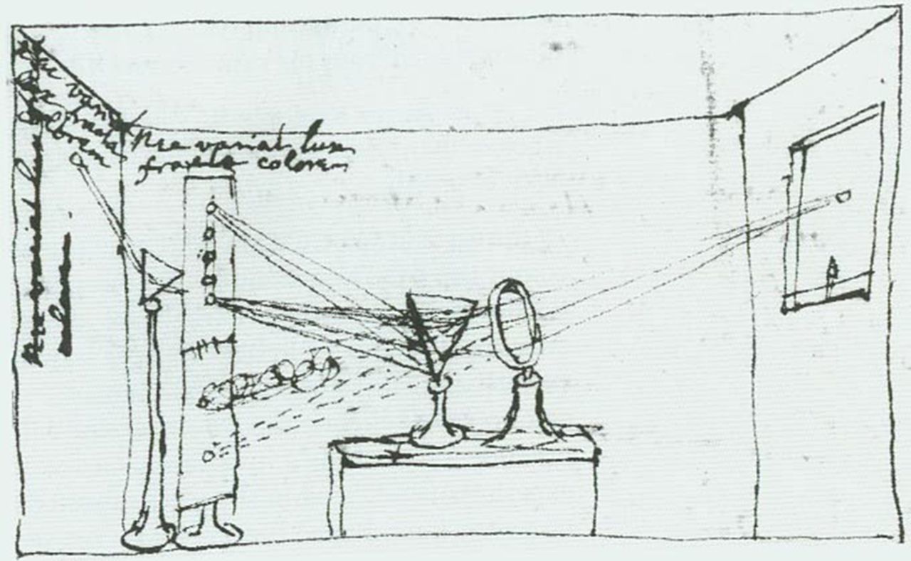
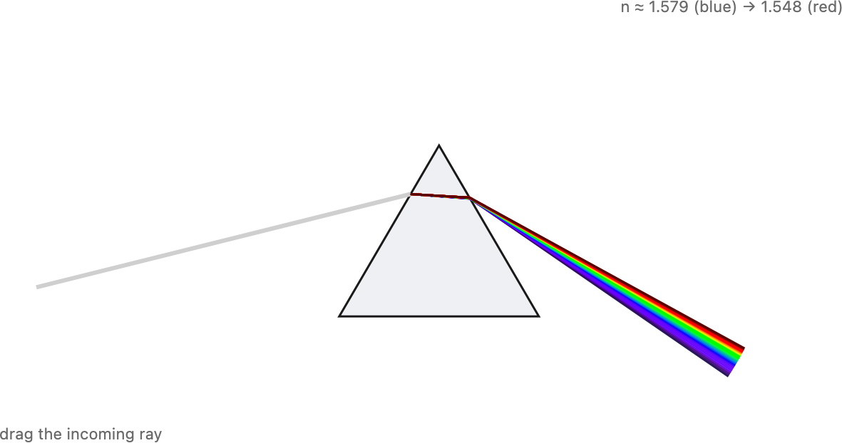
Newton's prism. The historical hook is Newton's prism experiment. Pass a beam of white sunlight through a glass prism and it fans out into the full spectrum — the rainbow band of pure colors. The crucial lesson is that white light is not a pure thing being "stained" by the glass; it is already a mixture of all wavelengths, and the prism merely bends each wavelength by a different amount, spreading the mixture out. Newton proved this with his experimentum crucis: he isolated one pure color from the spread and sent it through a second prism — and it did not split further. The pure colors are the irreducible ingredients; white is their sum (Figure 2.1.3).
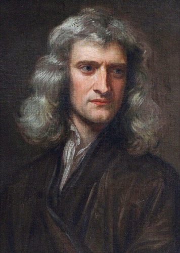 Isaac Newton (1642–1727) needs little introduction, but the prism is only the start of his presence in this book. The spectrum he split from white light is the physical basis of all the color science to come, and his Opticks established that color lives in the light, not the object. His corpuscular view of light competed for a century with the wave picture — both, we now know, are needed. On the mathematics side we still run Newton's method — step by the inverse curvature, $H^{-1}\nabla f$ — whenever a solver wants second-order convergence, and the Gauss–Newton refinement sits at the heart of feature tracking and bundle adjustment. Portrait: James Thornhill after Godfrey Kneller, 1689, public domain (via Wikimedia Commons).
So a spectrum is simply a function: power plotted against wavelength, $S(\lambda)$. You can think of it as an infinity of channels, one per wavelength. This matters enormously for everything that follows, because neither a camera nor the eye records all those channels — both keep only three numbers (the three cone types in the eye; the red, green, and blue filters in a camera). Collapsing an infinite spectrum down to three numbers is a drastic, lossy projection, and it is the root of metamerism: two physically different spectra can produce the identical three numbers and so look the same (taken up in detail in Color technology). For now, just hold the picture: light carries a whole spectrum, and we are about to throw most of it away.
2.1.2 Reflection, refraction, and what happens at a surface⧉
A camera sees nothing that has not first bounced off — or passed through — something. So before light reaches us it has interacted with matter, and three interactions cover almost everything: reflection, refraction, and diffraction (Figure 2.1.5).

Reflection is the simplest: a ray striking a smooth surface bounces off so that the angle going out equals the angle coming in, both measured from the surface normal ($\theta_i = \theta_r$). That single rule explains mirrors and, as we will see, the bright highlights on shiny objects.
Refraction is what happens when light crosses from one transparent medium into another — air into glass, air into water. Light travels more slowly in a denser medium, and the ratio of vacuum speed to the speed inside is the medium's refractive index $n$ (about 1.0 for air, 1.33 for water, 1.5 for typical glass). Because the wave slows, it bends, and the amount of bending follows Snell's law:
A good intuition is a marching band walking off pavement onto mud at an angle: the row hits the mud one end first, that end slows down while the other keeps marching, and the whole row pivots — the wavefront turns. Refraction is exactly this turning of a wavefront as one side slows before the other. You can watch it happen in an actual wave simulation (Figure 2.1.6): a plane wave crosses into a slower medium and its wavefronts both crowd together (the wavelength shortens by $1/n$) and bend toward the normal — Snell's law emerging from the wave equation rather than asserted, the wave-level companion to the diffraction simulation later in this chapter. It is also the entire reason a lens works; the fuller lens geometry is deferred to the Lens image formation chapter, but the bending rule is the same one here. Diffraction — the spreading of a wave at a small aperture — is the third interaction, and because it sets a fundamental resolution limit it gets its own section at the end of this chapter.

Light–matter interaction is largely resonance. It is worth pausing on why light slows in glass at all, and why materials have color: both come down to resonance. The wave's oscillating electric field drives the bound charges in a material — atoms, molecules, electrons tethered to their nuclei — and like any spring-loaded mass each has a natural frequency it most readily oscillates at. This is the Lorentz-oscillator picture, and almost everything optical follows from it. Near a resonance the driven charges swing hard and the material absorbs strongly, draining those wavelengths from the light; the wavelengths a material happens to absorb (and so remove from what it transmits or reflects) are exactly what give it its color. Away from resonance the charges still respond, just out of step, and that lag is what slows the wave — so the refractive index $n$ itself is a resonance effect. Because each wavelength sits a different distance from the nearest resonance, $n$ varies with wavelength — this is dispersion, $n(\lambda)$ — and that single fact is behind the prism fanning out a spectrum, the colors of a rainbow, and the chromatic aberration that plagues real lenses. That last consequence is not a footnote: because every glass disperses, a simple lens focuses blue and red at slightly different distances, and dispersion goes on to shape much of the challenge of lens design — the whole craft of combining crown and flint glasses into achromatic and apochromatic doublets, and the modern fight against chromatic aberration in fast lenses, exists to fight exactly this $n(\lambda)$ (developed in the Optics part). You can play with the whole resonance picture directly (Figure 2.1.7): drive the bound electron at different frequencies and watch the absorption peak at resonance and the refractive index swing through its normal-then-anomalous dispersion.

2.1.3 Polarization⧉
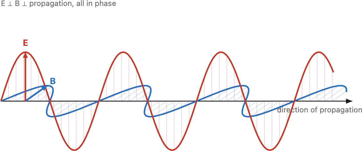
Light is a transverse wave: its electric field oscillates perpendicular to the direction the light travels. The orientation of that oscillation is the light's polarization. Natural light — from the sun, from a bulb — is unpolarized: the field direction is a rapidly varying jumble with no single preferred orientation. But reflection off a non-metallic surface (water, glass, a wet road, foliage) partially polarizes the reflected light, picking out one orientation. This is why a polarizing filter is so useful in photography: rotated to block that orientation, it cuts glare and reflections, lets you see into water, and deepens a blue sky (the sky's scattered light is partly polarized too). It is a physical effect you cannot replicate after the fact in software (forward-ref: the polarizer among the Photography 101 lens filters; reflection and specular removal in Single-image computational photography).
You meet polarization in two everyday places. First, good sunglasses are polarizers. The glare off a road, a lake, or a car hood is light that bounced off a roughly horizontal surface, so it comes out strongly horizontally polarized — most so at a particular Brewster's angle (the why lives in the reflection and BRDF material below). Quality sunglasses are linear polarizers oriented to pass vertical and block horizontal, so they kill that glare specifically — not just dim everything like a plain dark tint. That is the real difference between "good" (polarized) and merely cheap (just dark) sunglasses — and you can see it by rotating a pair over a glary surface (Figure 2.1.9). Second, LCD displays emit polarized light: an LCD forms its image by rotating polarization between two crossed polarizers, with the liquid-crystal layer acting as a per-pixel shutter. That is why polarized sunglasses can make some screens go oddly dark — or shift color — when you tilt your head.

Both follow from Rayleigh scattering: air molecules are much smaller than the wavelength of light and scatter short (blue) wavelengths far more strongly than long (red) ones — the scattered fraction grows as $1/\lambda^4$, so blue (≈450 nm) scatters roughly ten times more than red (≈650 nm). At midday the sunlight takes a short path through the atmosphere; the blue it sheds is scattered out in every direction and reaches your eye from all over the sky, so the sky reads blue while the sun stays roughly white. At sunset the light skims a long, grazing path through the air; by the time it reaches you almost all its blue has been scattered away, and mostly orange and red survive — so the sun and the clouds near it redden (Figure 2.1.10). When the scattering particles are large compared to the wavelength — water droplets in fog or cloud — every wavelength scatters about equally (Mie scattering), which is why clouds and haze are white or gray, not blue. Minnaert, The Nature of Light and Colour in the Open Air

A rainbow is, surprisingly, a caustic — a place where light piles up. It is tempting to explain it as "dispersion, like Newton's prism," but dispersion alone is not a rainbow: a prism merely fans white light into a spread, and a spread is not a bright arc pinned at a fixed angle. The brightness and the fixed 42° angle come from the geometry of the sphere; dispersion only supplies the colours. Each falling raindrop is a tiny sphere, and sunlight refracts in, reflects once off the back, and refracts out again (Figure 2.1.11, left).
Here is the heart of it. Slide the entry point across the drop — the impact parameter — and the total deviation of the exiting ray sweeps down to a minimum (about 138° for water) and turns back up. Near that minimum the deviation is stationary, so rays entering at many different points all leave in almost the same direction: they bunch up, and that pile-up is the bright arc, seen at $180°-138° \approx$ 42° from the antisolar point (Figure 2.1.11, right). This is why the single internal reflection is essential — and why a ray that only refracts in and out, with no bounce, makes no rainbow at all: with two refractions only, the deviation grows monotonically with the impact parameter and never turns around, so there is no stationary angle for light to concentrate at. The primary bow is the one-bounce caustic at 42°; the fainter, colour-reversed secondary bow is the two-bounce caustic, its own minimum putting it at about 51°. Only now does dispersion matter: because $n$ is a touch larger toward the blue, each colour's caustic sits a degree or so from its neighbours, fanning the bunched light into the ordered band we see.
Between the two bows sits a conspicuously darker strip of sky, Alexander's band (named for Alexander of Aphrodisias, who described it around 200 AD). Its darkness follows directly from the caustic story: one-reflection light only ever emerges at 42° or less — it piles up at 42° and scatters out to fill the sky inside the primary bow — while two-reflection light only emerges at 51° or more, outside the secondary. The 42°–51° gap between them receives almost no rainbow light from either path, so it reads as a dark band, with brighter sky on both sides. You can see the whole story in a real double bow over Loch Ness (Figure 2.1.14): bright primary, fainter reversed secondary outside it, the dark band between, and the noticeably brighter sky inside the primary.
You can run the whole experiment on a workbench with a clear glass sphere standing in for a raindrop (Figure 2.1.12): a bright beam refracts in, reflects off the back, and throws a little rainbow caustic onto a card. Send narrow laser beams through the same sphere in a hazy room and the rays themselves become visible (Figure 2.1.13): you can watch each beam refract in, bounce off the back, and refract out — the exact refract–reflect–refract path the diagram traces. The rainbow in the sky is just this single-drop geometry, summed over a skyful of drops. Minnaert, The Nature of Light and Colour in the Open Air

Why a drop makes a bow and a prism does not. Left: parallel sunlight enters a spherical water drop at different points, refracts, reflects once off the back, and exits bunched near the 42° rainbow ray — a caustic. A ray that only refracts through (no internal reflection) just passes on, turned but never concentrated. Middle: Descartes' construction — total deviation $D$ versus impact parameter $b$. The one-reflection curve has a minimum (≈138° → a bow at 42°); two reflections give the secondary (≈51°); the zero-reflection curve (two refractions only) is monotonic — no minimum, no caustic, no rainbow. Right: the same physics as an integral — the ray density as a function of deviation (summed over every impact parameter), which spikes exactly at the stationary deviation: that spike is the rainbow, and dispersion splits it into the three coloured spikes shown. Interactive: it is a water drop; drag the impact parameter, choose the number of internal reflections, and tick "zoom near the caustic" to re-range both the slider and the plot tightly around the bow. Dispersion is always on, so the colours separate near the minimum.
Stands alone: a ray traced through a spherical drop beside the deviation-vs-impact-parameter plot, showing the rainbow as the stationary (minimum-deviation) angle of the one-internal-reflection ray, and no caustic for the two-refractions-only path.


Scattering and absorption in media. The same physics that paints the sky operates at close range whenever light travels through a participating medium — fog, haze, smoke, or water. Light is scattered out of its straight path and absorbed along the way, so distant objects lose contrast and take on the color of the medium (the bluish veil of haze, the green-blue cast underwater). When light scatters only once before reaching the camera the effect is mild; multiple scattering through thick fog washes the scene out entirely. Undoing this — dehazing and de-weathering — is a recurring computational-photography problem, and it is built on exactly the scattering model sketched here.
2.1.4 The color of objects: illumination times reflectance⧉
Here is a fact that sounds obvious but has deep consequences: a red apple is not red in the dark. An object has no color of its own to emit; it only reflects whatever light falls on it. So the color that reaches your eye is the result of two spectra multiplied together, wavelength by wavelength:
Here $S(\lambda)$ is the illuminant — the spectrum of the light source actually present — and $\rho(\lambda)$ is the surface's spectral reflectance, the fraction of light it sends back at each wavelength. Reflectance is the object's intrinsic, fixed signature: the apple's $\rho(\lambda)$ is high in the reds and low in the greens and blues, whatever the lighting. Illumination is whatever happens to be shining. Their per-wavelength product is what leaves the surface and reaches the eye (Figure 2.1.15). A red apple under white light reflects mostly red; the same apple under pure green light has almost nothing to reflect and looks nearly black — its reflectance is real, but there is no red illumination for it to act on.

This multiplicative entanglement is profound, and it is the first instance of a principle that runs through the whole book.
Much of imaging is multiplicative, not additive. The light reaching the eye is illumination times reflectance; contrast is a ratio of intensities; a shadow darkens a region by a factor, not by subtracting a constant. Because the structure is multiplicative, the natural tools are multiply, divide, and log — not just add. This is why, again and again, we will work with ratios and with logarithmic encodings rather than raw linear values. It is also why white balance is hard: to recover an object's true color we must divide out the unknown illuminant $S(\lambda)$ from the product $C(\lambda)$ — undoing a multiplication we never observed directly. (The additive counterpoint — light from different sources adding — and what it means for choosing an encoding, comes in Color technology.)
A caveat on scope: the clean product $C(\lambda) = S(\lambda)\rho(\lambda)$ assumes the surface reflects the same in every direction — the matte, or Lambertian, case, where a single reflectance number per wavelength suffices. Real surfaces are directional: a shiny apple has a bright highlight that moves as you move. Capturing that direction-dependence requires a richer object than a single $\rho(\lambda)$, and that is the BRDF, next.
2.1.5 The BRDF and the look of materials⧉
To describe how a real surface reflects, we need a function that knows about directions — both where the light comes from and where the viewer looks from. That function is the bidirectional reflectance distribution function (BRDF). For a point $p$ on a surface with normal $\mathbf{n}$, the BRDF $f_r$ says how much of the light arriving from one direction is re-emitted toward another:
The "bidirectional" in the name is the whole point: the reflected radiance toward a viewer at $q$ depends on both the incoming direction and the outgoing direction (and on wavelength, which is why surfaces are colored). The BRDF is, in effect, the complete optical fingerprint of a material — give a renderer the BRDF and it can show you that material under any lighting and from any angle (Figure 2.1.16).

Diffuse versus specular. Two idealized extremes anchor the whole range of materials (Figure 2.1.17). A diffuse, or Lambertian, surface — chalk, matte paint, paper — scatters incoming light into a broad lobe, sending it nearly equally in all directions. Its key, slightly counterintuitive property is that it looks equally bright from every viewpoint: walk around a matte ball and its shading does not change with your position. (What does change its brightness is the angle of the light, which dims as $\cos\theta$ — a fact we make precise in the radiometry section.) A specular, or shiny, surface — polished metal, glass, a wet apple — does the opposite: it concentrates reflection into a tight lobe near the mirror direction, producing a sharp highlight that is view-dependent and slides across the surface as you move. Most real materials are a blend: a diffuse base color plus a specular sheen — which is exactly how computer-graphics shading models combine them.

Polarization, again. There is one more thing the BRDF leaves out if we treat reflectance as a single directional number: the light–matter interaction also polarizes the light. As the polarization sidebar above noted, reflection — especially the specular component — partially polarizes what bounces off a surface, with the effect strongest near Brewster's angle. A truly complete account of reflection is therefore polarization-dependent: the BRDF becomes a polarization BRDF, or pBRDF, tracking not just how much light goes where but how its oscillation orientation is reshaped on the way. This is exactly the handle a polarizing filter grabs (Photography 101 — lens filters), and it is what shape-from-polarization and reflection-removal methods exploit to read surface orientation or strip away glare (Advanced).
A BRDF is per-wavelength: the same wavelength goes in and comes out, merely redistributed in direction, so a surface is one BRDF for the reds, another for the blues, and they never talk to each other. Fluorescence violates this. A fluorescent material absorbs short-wavelength light — often ultraviolet — and re-emits it at longer wavelengths, the shift toward red called the Stokes shift. Energy is moved between wavelengths, so the material is no longer described by a scalar BRDF per $\lambda$ but by a bispectral reradiation matrix that maps an input wavelength to an output wavelength. (This is also why a fluorescent surface can appear to reflect more than 100% of the light in its emission band — it is borrowing energy from the ultraviolet you cannot see.) Once you look for it, fluorescence is everywhere: the optical brighteners that make detergent and paper look "whiter than white," highlighter ink, minerals glowing under a UV lamp, green fluorescent protein (GFP) in cell biology, and the hidden security inks in banknotes — and it is the working signal of fluorescence microscopy and forensics.
A BRDF makes one more quiet assumption: that light leaves a surface at the same point it entered. In translucent materials this fails. Light enters, scatters around beneath the surface, and exits somewhere else, so a point-wise BRDF is simply insufficient — what you need is a BSSRDF, the bidirectional surface-scattering reflectance distribution function, which couples a separate entry point to an exit point. Skin, marble, milk, wax, and leaves all do this. It is what gives skin its soft, "lit-from-within" glow and its gently rounded shadow terminator; render skin with a pure BRDF and it looks unmistakably plastic. (Cross-ref: translucency in physically based rendering.)
Global illumination. One more complication, mentioned now and developed later: light rarely bounces only once. It ricochets between surfaces many times, so the light "arriving" at a point is not just the source but also the light reflected off everything else in the scene. A vivid symptom is color bleeding — a red wall casts a faint red tint onto a white floor beside it (Figure 2.1.18). Accounting for all these bounces is global illumination, the foundation of physically based rendering; here we only flag that the light striking a surface already carries the color of its surroundings.

2.1.6 Illuminants⧉
We have been treating "white light" as a single thing, but it is not. The light at noon, the light at sunset, the light from a tungsten bulb, and the light from a fluorescent tube all have very different spectra $S(\lambda)$, and since the stimulus reaching the eye is the product $S(\lambda)\rho(\lambda)$, the same scene genuinely sends different colors to the eye under each.
The most useful organizing idea is the blackbody: an ideal hot object whose emitted spectrum is fixed entirely by its temperature. As it heats, it glows first dull red, then orange, yellow, white, and finally bluish — exactly the sequence a heated iron bar runs through. This gives us color temperature, quoted in kelvin (K), as a one-number handle on the color of a light (Figure 2.1.19). The convention is, confusingly, backwards from everyday usage: low color temperatures (~3000 K) are warm, orange-ish; high ones (~6500 K and up) are cool, bluish. Standard reference illuminants include D65 (≈6500 K, a model of average daylight, the basis of most color standards), tungsten (≈3200 K, the warm glow of an incandescent bulb), and fluorescent lighting — which is not a smooth blackbody curve at all but a spiky spectrum with sharp emission lines, which is why fluorescent light renders some colors poorly and gives photos an unpleasant cast.

The lesson, restated, is the one from L1: because the stimulus is the spectral product of illuminant and reflectance, a surface's apparent color is never absolute — it shifts with the light. Our visual system silently compensates (a white shirt looks white indoors and out), and a camera must do the same compensation explicitly. That compensation is white balance, and recovering it — dividing out the illuminant — is one of the central problems of Color technology.
2.1.7 Radiometry: radiance, irradiance, exposure, and falloff⧉
So far we have tracked light's color. Now we track its energy — how much light a ray carries and how much of it lands on a sensor. This is radiometry, and getting two of its quantities straight prevents a great deal of confusion later.
Radiance. The fundamental quantity a pixel ultimately measures is radiance $L$: the power travelling along a single ray, per unit area and per unit solid angle (solid angle — the 2-D analogue of an angle, measuring how big a cone is — is treated in the appendix). The essential and surprising property of radiance is that it is conserved along a ray as it travels through empty space: it does not fall off with distance (Figure 2.1.20). A blank white wall does not get dimmer as you step away from it — it only gets smaller in your field of view. Each individual ray from the wall carries the same radiance no matter how far it has travelled; there are simply fewer of those rays landing in each pixel as the wall shrinks. Hold onto this: radiance is distance-invariant, and it is the quantity scenes are made of.

Irradiance. What a sensor actually accumulates is irradiance $E$: the power per unit area arriving on a surface, gathered from all the directions that reach it. It is the integral of incoming radiance over the collecting solid angle,
and unlike radiance it does depend on the geometry of collection: a wider lens aperture gathers a larger solid angle and so collects more irradiance. That is the radiometric reason a faster lens makes a brighter image.
The cosine law. The $\cos\theta$ inside that integral is not a fudge factor; it is projected area (Figure 2.1.21). Picture a cylindrical beam of light — a shaft of width $w$ — striking a surface. If it hits head-on, it illuminates a patch of width $w$. If it hits at an angle $\theta$ from the normal, the same beam spreads over a longer footprint $w/\cos\theta$, so the same power is smeared over more area and the irradiance is thinned by $\cos\theta$. This is Lambert's cosine law: a surface tilted away from the light receives less light per unit area, in proportion to $\cos\theta$. It is why a Lambertian sphere fades smoothly toward its edges.

The cosine law explains the seasons, and it is not about distance from the sun (Earth is actually slightly closer to the sun in the northern winter). The Earth's axis is tilted 23.5°. In summer the noon sun stands high and its rays strike the ground near vertically — concentrated, full strength. In winter the noon sun is low and the same rays arrive at a grazing angle, spreading the same power over a larger patch of ground — by the cosine law, roughly half the energy per unit area. Summer is warm because sunlight is concentrated, not because we are nearer the sun (Figure 2.1.22).

Radiometric versus photometric units. Worth pinning down before we go on: everything above is radiometric — raw energy, measured in watts. But the eye does not weigh all wavelengths equally, and the photographic and display worlds quote a parallel set of photometric units that fold in the eye's spectral sensitivity, the luminous-efficiency curve $V(\lambda)$. Weight a radiometric quantity by $V(\lambda)$ and integrate over wavelength and you get its photometric twin: radiant flux in watts becomes luminous flux in lumens (lm); irradiance in W/m² becomes illuminance in lux (lm/m², what an incident light meter reads); radiance in W/m²/sr becomes luminance in cd/m² — the "nit" — and intensity in W/sr becomes luminous intensity in candela (cd), which is the SI base unit (roughly the output of one candle). The chain is consistent: $\text{cd/m}^2 = \text{lm}/(\text{m}^2\cdot\text{sr})$. Luminance, cd/m², is the one to remember: it is the perceptual "brightness" of a patch, and it is the unit displays and HDR are specified in and the axis the photopic/scotopic perception scale lives on. For a sense of scale, a typical monitor runs ~100–300 cd/m², an HDR display reaches 1000+, and white paper in direct sunlight is around $10^4$ cd/m².
Exposure. The total light a sensor collects is irradiance accumulated over the shutter time $t$:
This exposure $H$ is the actual quantity that fills the photosites. It ties directly to the two controls a photographer turns: irradiance grows with aperture (a bigger opening gathers more solid angle — the dependence is on $(D/f)^2$), and the integration runs for the shutter time $t$. Those controls, and the noise that accompanies the count, are the subject of the next chapter (Image formation and linear perspective).
Falloff — and the classic confusion. Now the part that trips people up. A point source — a bare bulb, a star — does fall off as the inverse square of distance, $E \propto 1/r^2$: its light spreads over a sphere whose area grows as $r^2$, so the irradiance on anything it lights drops as $1/r^2$. This is real and familiar — a flash is far brighter up close. But scene radiance is distance-invariant — the wall does not dim. How can both be true? The resolution is that they describe different things: $1/r^2$ governs the irradiance a point source delivers, while distance-invariance governs the radiance of an extended surface as seen along a ray (Figure 2.1.23). The surface's radiance stays constant; what shrinks is its angular size, not its brightness. Keep these two straight — the literature is littered with confusion that comes from conflating them.

This radiometric bookkeeping is what later chapters build on. Recovering the true scene radiance from one or several photographs is the goal of high dynamic range (HDR) imaging; deliberately controlling the illumination to learn about a scene is computational illumination. (One more piece of falloff — the gentle $\cos^4\theta$ dimming toward the corners of a frame, or natural vignetting — is deferred to the Sensors chapter, where a finite aperture and a real pixel make it meaningful.)
2.1.8 Wave effects, diffraction, and the diffraction limit⧉
We end where we began, with the wave picture — because it imposes a hard limit on every lens ever made. When light passes through a small aperture or skims a sharp edge, it does not continue in perfectly straight rays: it diffracts, bending and spreading out. And, counterintuitively, the smaller the aperture, the more the light spreads (Figure 2.1.24). A wide opening lets the wavefront through almost undisturbed; a narrow one forces it to fan out, through an angle of roughly $\theta \approx \lambda / D$ for an aperture of diameter $D$.

Where does that spreading come from? It is purely a property of waves, and we can watch it happen by solving the wave equation directly. Send a flat wavefront at an opaque barrier with a single slit and let the wave evolve in time: in front of the slit the wavefronts stay flat, but the moment they pass through, they bow into expanding circular arcs and fan outward (Figure 2.1.25). Narrow the slit relative to the wavelength and the fan opens wider — exactly the $\theta \approx \lambda / D$ behaviour, now as an emergent consequence of the wave dynamics rather than a rule asserted.

The Airy disk. The consequence for imaging is unavoidable: a finite aperture cannot focus light to a perfect point. Even a flawless, aberration-free lens images a single distant point not as a point but as a small bright blur surrounded by faint rings — the Airy disk — whose angular radius is
giving a blur-spot diameter on the order of $2.44\,\lambda N$, where $N = f/D$ is the lens's f-number (Figure 2.1.26). The Airy disk is the diffraction-limited point-spread function: the smallest spot any lens of that aperture can produce, set by wavelength and f-number alone.

The diffraction limit. Because two nearby point sources blur into two overlapping Airy disks, there is a finest detail a lens can resolve — the diffraction limit. By the Rayleigh criterion, two points are just resolvable when the center of one Airy disk falls on the first dark ring of the other, again at $\theta \approx 1.22\,\lambda/D$. The headline is that a larger aperture diffracts less and resolves finer detail.
This produces the photographer's sweet spot. Open the aperture wide and aberrations (the imperfections of real glass, deferred to the Optics part) dominate, softening the image. Stop the aperture far down and diffraction dominates, softening it again. Somewhere in between — typically a couple of stops down from wide open — the two effects are jointly minimized and the lens is at its sharpest. "Stopping down too far softens the image" is not a defect of cheap lenses; it is physics, and the trade-off is made quantitative with the modulation transfer function in the Optics part.
Finally, a scope note that justifies most of the book. We will almost always assume incoherent light — the everyday case of sunlight and bulbs, where light from different points is uncorrelated, so intensities simply add, stay positive, and combine linearly. That linearity is what makes ordinary image processing tractable. Coherent light (lasers) and full wave optics — where amplitudes add and can cancel — return only for the advanced topics of metalenses, lensless cameras, and holography. With that, we have followed light from its source, off a surface, and to the edge of the camera; the next chapter takes it through the aperture and onto the sensor.
Big lessons of this chapter
The recurring principles from this chapter, gathered for review.
Much of imaging is multiplicative, not additive. The light reaching the eye is illumination times reflectance; contrast is a ratio of intensities; a shadow darkens a region by a factor, not by subtracting a constant. Because the structure is multiplicative, the natural tools are multiply, divide, and log — not just add. This is why, again and again, we will work with ratios and with logarithmic encodings rather than raw linear values. It is also why white balance is hard: to recover an object's true color we must divide out the unknown illuminant $S(\lambda)$ from the product $C(\lambda)$ — undoing a multiplication we never observed directly. (The additive counterpoint — light from different sources adding — and what it means for choosing an encoding, comes in Color technology.)