5.1 Poisson image editing🔗⧉

Cut a toucan out of one photo and drop it into another — onto a branch in a different forest, say. Paste the bird's pixels onto the new background and the composite fails in one very specific way: a crisp halo runs all the way around the toucan, exactly where its pixels abut the new scene's. The bird was lit by a different sun, white-balanced by a different camera, and exposed a touch differently, and every one of those mismatches becomes a sudden jump in brightness and color right at the boundary. The interior of the toucan looks perfect. It is the seam that betrays the forgery.

The obvious patch — feathering, where you blur the boundary so the two images cross-fade — does not really work. A blur has a single scale, so it either leaves the broad color mismatch plainly visible or it smears the toucan's beak into the leaves behind it. What we actually want is for the pasted bird to flow out of its new surroundings: to keep its own texture and shading but adopt the new scene's local color and light at the rim, so that there is simply no jump for the eye to catch. Astonishingly, that — and a whole zoo of other seamless edits — drops out of one idea: do not edit the pixels; edit their gradients, then reconstruct the image whose gradients best match.

That idea is this chapter. We will pose the reconstruction as the Poisson equation, recognize it as the same large, sparse least-squares system we met in regression, and then watch an entire family of edits — seamless cloning, the healing brush, gradient-domain high dynamic range (HDR), photomontage — appear by changing nothing but the gradient field we ask the image to match.

5.1.1 The key idea: edit gradients, not pixels🔗⧉

Here is the single observation the whole chapter stands on. The human visual system is far more sensitive to local contrast — how much a pixel differs from its neighbors — than to any pixel's absolute value. What makes the toucan look like a toucan is not that one patch of its beak happens to be RGB $(0.91, 0.43, 0.08)$; it is that there is a sharp transition from a dark feather to a bright beak right here. The absolute level is free to drift — a whole region can grow lighter or pick up a color cast — and as long as the differences between neighbors survive, the eye reads the same scene. This is precisely why lightness constancy works: we judge a surface by its contrast against its surroundings, not by the raw quantity of light reaching us. A sheet of paper looks white in deep shade and in full sun even though the shadowed paper sends our eye far less light than a sunlit lump of coal sends from the next room.

So we move our object of manipulation from the image to its gradient field. Write $\mathbf{v}$ for the gradient field we want the answer to have — the guidance field — and $f$ for the image we solve for. Ideally $\nabla f = \mathbf{v}$ everywhere. The catch, unpacked in the sidebar just below, is that this is almost never exactly solvable: a field of two numbers per pixel is generally not the gradient of any single image. So we settle for the next best thing and ask for the image whose gradients come closest, in the least-squares sense:

Read back in words: find the image $f$ whose gradients deviate as little as possible, summed over the whole image, from the gradient field we prescribed. This is exactly an inverse problem of the kind in Linear Inverse Problems and Regression — a quadratic energy in the unknown image — and minimizing a quadratic means setting its derivative to zero, which gives a linear system. That system is the Poisson equation,

where $\nabla^2$ is the Laplacian (the second-derivative operator) and $\operatorname{div}\mathbf{v}$ is the divergence of the guidance field — the net outflow of a vector field; if divergence is rusty, see Refreshers → Calculus. We derive the discrete form in the next section; for now keep its shape in view: we ask that the Laplacian of the output match the divergence of the field we prescribed. When $\mathbf{v}$ really is the gradient of some source image $g$, this just says the output's Laplacian should equal the source's, since $\operatorname{div}\nabla g = \nabla^2 g$.

5.1.2 Seamless cloning: the headline application🔗⧉

The toucan-into-the-forest problem now has a clean recipe, due to Pérez, Gangnet and Blake (2003), and it is worth stating exactly, because everything else in the chapter is a variation on it. We have a destination image $f^{*}$, a source image $g$, and a region $\Omega$ (the mask) where we want to paste. Rather than copy the source's pixels into $\Omega$, we copy its gradients — set the guidance field to $\mathbf{v} = \nabla g$ inside $\Omega$ — and we solve for the interior values $f$ that best match those gradients, subject to one constraint: at the boundary $\partial\Omega$ of the region, $f$ must equal the destination. That boundary constraint is a Dirichlet condition,

read back as: pin the edge of the pasted region to the surrounding image's actual pixel values. Inside, solving $\nabla^2 f = \operatorname{div}\mathbf{v}$ fills in values that carry the source's contrasts — the toucan's feathers, the gloss of its beak — yet flow smoothly out of the destination at the seam.

Why does this kill the seam? Because the only freedom the solver retains is the absolute level, and it spends that freedom satisfying the boundary. If the source patch is, say, two stops brighter than where we drop it, the naive copy makes that two-stop jump visible all the way around the rim. The gradient version never commits to the source's brightness at all; it commits to the source's differences and lets the boundary set the level, so the whole patch slides in tone and color until it matches its new surroundings exactly at the edge, with no jump left to see. The lighting and color mismatch is absorbed, not hidden (Figure 5.1.1).

There is an honest way to see what the solver is doing, and it pays off later. Suppose for a moment the destination's boundary values happened to coincide with the source's. Then copying the gradients would simply reproduce the source — no jump, done. In general they do not coincide, so think about the discrepancy: at each boundary point there is a difference between what the destination wants ($f^{*}$) and what the source provides ($g$). The Poisson solve quietly spreads that boundary discrepancy smoothly across the interior — it adds a gentle correction surface, large where the mismatch is large and dying away inward — so the patch keeps the source's gradients exactly while absorbing the level difference as a soft, invisible gradient of its own. We will name that correction surface — the membrane — and exploit it for speed near the end of the chapter.

A note on encoding, following our standing rule of declaring the space every edit lives in: for an ordinary clone where source and destination are similarly exposed, the usual gamma values are fine. But when the tones or exposures differ substantially — and especially for gradient-domain HDR — we integrate in log, for reasons made precise in the next section.

5.1.3 Reconstruction = solving the Poisson equation🔗⧉

To turn $\nabla^2 f = \operatorname{div}\mathbf{v}$ into something a computer can solve, we discretize it, and the discretization is satisfyingly plain. Approximate the gradient with finite differences — the difference between a pixel and its left neighbor, and between a pixel and its top neighbor. We deliberately use the simplest kernels, $[-1,\,1]$ and its vertical transpose, not the wider Sobel kernels: Sobel is tuned for analyzing gradients and averages over too large a support, whereas here we want to stay as close as possible to the raw pixel differences.

Now compose them. The Laplacian is the gradient followed by (minus) the gradient again — a second derivative — and convolving $[-1,1]$ with its flip gives the familiar 1-D stencil $[-1,\,2,\,-1]$; summing the horizontal and vertical contributions gives the 5-point Laplacian, which subtracts each pixel's four neighbors from four times itself. Plugging that in, the Poisson equation becomes one linear equation per pixel $p$ over its four neighbors $N(p)$:

where $v_{pq}$ is the prescribed difference across the edge from $p$ to its neighbor $q$ (for a clone, $v_{pq}=g_p-g_q$, the source's own difference). A note on the sign convention. We use the positive discrete Laplacian, $|N_p|\,f_p-\sum_{q} f_q$ — the standard $[-1,2,-1]$ stencil — which approximates $-\partial^2/\partial x^2$, the negative of the continuous operator. Under this convention both sides of the continuous identity $\nabla^2 f=\operatorname{div}\mathbf v$ flip sign together, so the linear system above is unchanged; this matches Pérez. Read the equation back: each pixel's value, minus the sum of its neighbors, should equal the divergence of the guidance field there. Stack one such equation per pixel and you have a large, sparse, structured linear system — sparse because each equation touches only five pixels, structured because every row is the same Laplacian stencil, just shifted (a convolution). Only the right-hand side depends on the guidance field; the matrix does not.

The system needs boundary conditions to be well-posed, and which one you use depends on the task. For cloning we already have it: the Dirichlet condition $f|_{\partial\Omega}=f^{*}|_{\partial\Omega}$ pins the region's boundary to the destination. When instead we integrate a guidance field over a whole image with no enclosing destination — gradient-domain HDR, for instance — there is no boundary to pin, and we use a Neumann condition (zero normal derivative at the image border), which fixes the overall brightness only up to a constant.

The single equation per pixel already hands us the most transparent way to solve the system. Solve the per-pixel relation $4 f_p - \sum_{q\in N(p)} f_q = b_p$ for $f_p$ — where $b_p = \sum_{q\in N(p)} v_{pq}$ is the divergence right-hand side, computed once — and each pixel is just the average of its four neighbors plus a quarter of $b_p$. Sweep that update over every interior pixel, holding the boundary fixed, and repeat until the image stops changing:

b[p] = ∑ over q in N(p) of v[p, q]      # divergence, computed once
initialize f (e.g. f = destination, or zero in the interior)
while not converged:
    for each interior pixel p:
        f[p] = ¼ · (∑ over q in N(p) of f[q] + b[p])
    keep f fixed on the boundary
return f

Read it back: each pass nudges every pixel toward the average of its neighbors, carrying the prescribed divergence with it. This is the Jacobi / Gauss-Seidel iteration, and it is correct but slow — it propagates information inward from the boundary one pixel-ring per sweep, so a large region takes many passes to settle. That sluggishness is exactly what the better solvers below fix. As a sanity check on the whole construction, set the guidance field to zero ($\mathbf{v}=0$): the Poisson equation collapses to Laplace's equation $\nabla^2 f = 0$, whose solution inside a region, with the boundary pinned, is the smoothest possible interpolation of the boundary values — a membrane stretched across the hole. In 1-D that membrane is just a straight line between the two endpoints; in 2-D it is the soap-film surface those boundary values support. Hold onto that membrane; it returns.

The same solver as the regression chapter🔗⧉

The crucial practical point is the one we already made for deblurring: do not form the matrix. Stacking every pixel into a vector and building the Laplacian as an explicit matrix would be enormous and pointless. Instead we keep the image as an image and use the abstract linear algebra only to tell us what operations to perform — and every one of them turns out to be a simple image operation. Applying the Laplacian "matrix" to the current guess is just convolving with the 5-point stencil; the right-hand side is the divergence of the guidance field, computed once; the inner products the iterative solvers need are just sums of pixelwise products. So the entire solve reduces to repeated convolutions, a few image dot products, and some scalar arithmetic — never a matrix in sight.

This is exactly the machinery of Linear Inverse Problems and Regression, and the same three solver choices apply:

• Conjugate gradient (CG), optionally with a preconditioner — the workhorse. It only ever needs to apply the Laplacian to a vector (a convolution), it exploits the system's sparsity and symmetry, and it converges far faster than plain gradient descent, which crawls because it propagates information inward from the boundary one pixel-ring at a time and tends to zigzag.
• Multigrid — coarse-to-fine, solving on a small image first and refining down the pyramid, which fixes precisely gradient descent's slow long-range propagation. This is the pyramid idea of Linear pyramids and wavelets put to work as a solver.
• An FFT solver on a rectangular periodic or Neumann domain. The Laplacian is a convolution, and convolution diagonalizes in Fourier (the sine waves are its eigenvectors), so the Poisson solve becomes a per-frequency division — one FFT, a divide, one inverse FFT. This ties straight back to Linearity, Fourier, Aliasing and deblurring.

It is the same sparse, symmetric, positive-definite system that shows up in colorization, matting, and regularized deblurring — learn to solve it once and you have solved all of them.

The FFT route deserves a closer look, because it is the cleanest instance of a lesson we have leaned on before. Both the gradient and the Laplacian are convolutions — linear and shift-invariant — and any shift-invariant operator is diagonal in the Fourier basis: it does nothing but scale each frequency. On a rectangular domain with periodic (or Neumann) boundaries the Poisson equation $\nabla^2 f = \operatorname{div}\mathbf{v}$ therefore decouples completely — every frequency is its own independent scalar equation — and the whole solve collapses to one per-frequency division,

where $\widehat{\nabla^2}(\omega) = -(\omega_x^2+\omega_y^2)$ is the Laplacian's spectrum (Figure 5.1.3). One forward FFT of the divergence field, one pointwise divide by that spectrum, one inverse FFT, and we are done — no iteration at all. This is exactly the "diagonalize when you can" (L5) FFT solver we used for deblurring (see Efficient solvers / Linearity, Fourier, Aliasing and deblurring): wherever the operator is a convolution and the domain is a clean rectangle, Fourier turns a giant linear system into a single elementwise division. (When the boundary is free rather than periodic — the Neumann/zero-normal-derivative case — the DCT, the cosine cousin of the FFT, plays the same role with the right boundary behavior.) There is one subtlety worth flagging, and it is the same zero-eigenvalue we keep meeting: at $\omega=0$ the spectrum $-(\omega_x^2+\omega_y^2)$ vanishes, so the division is undefined for the DC term — the image's overall mean. This is not a numerical accident but the statement that gradients pin down everything except the absolute level: shift the whole image up by a constant and its gradients, divergence, and Laplacian are all unchanged. The mean is left free, exactly as L9 promises, and must be set separately — by a boundary value, or by simply choosing a reference. It is the same undetermined offset the membrane absorbs in the cloning case, seen now from the frequency side.

Which space to integrate in: linear vs. gamma vs. log🔗⧉

By our encoding-clarity rule, every edit must declare the space it works in, and for Poisson editing the choice genuinely matters. The principle is simple: integrate in a space where equal gradients mean equal perceived contrast.

Plain linear light is the wrong choice when tones are mismatched. Contrast is fundamentally a multiplicative quantity — a step from 100 to 200 units of light and a step from 1000 to 2000 look like the same contrast to us, but in linear light the second has ten times the gradient. So a linear Poisson solve over-weights the highlights: bright regions dominate the seam, and pasting a patch from a dark area into a bright one loses contrast because the solver is trying to reproduce linear differences that no longer correspond to what the patch should look like. The results come out flat and pastel.

The fix is to work in log. A ratio becomes a fixed difference in the log domain — $\log 200 - \log 100 = \log 2000 - \log 1000$ — so a multiplicative contrast maps to a constant gradient, which is exactly what the eye reads and what keeps shadow detail alive. (The one caution is the usual one with logs: guard against zeros by adding a small constant before taking the log.) So for tone- or exposure-mismatched clones, and for gradient-domain HDR, we take gradients and integrate in log, then map back to display. For everyday similarly-exposed clones, gamma is adequate. The general lesson — integrate where the metric matches perception — is just what the next point refines for color.

A perception-based color space🔗⧉

The linear-versus-log point is really a special case of a broader question: in what representation does gradient magnitude best track perceived contrast? Hamilton Chong, Steven Gortler and Todd Zickler (2008) answer it for color, building a color space designed so that the gradient's magnitude is covariant with perceived contrast — a perception-based, illumination-invariant space in which to take and integrate gradients. Doing the Poisson solve there is the best-behaved choice when color, not just luminance, is at stake; it generalizes "use log" from a single channel to the full color manifold. We will not need its machinery, but it is the principled endpoint of the encoding discussion: choose the space so that the thing you are matching — the gradient — means the same to the math as it does to the eye.

5.1.4 Poisson vs. pyramid blending🔗⧉

That membrane is also the cleanest lens on how Poisson blending differs from the other classic seam-hider, Laplacian-pyramid blending (the multiresolution spline, Burt & Adelson 1983 (spline blending)). Both make a paste seamless by treating slow variation differently from fine detail — but they part on a single point: what becomes of the source's absolute level, its DC.

Poisson is gradient-domain with a pinned boundary. It reproduces the source's gradients and lets the membrane absorb whatever offset the boundary demands, so the source's DC is discarded and re-set by the destination — adding a constant to the source changes nothing. Laplacian-pyramid blending instead cross-fades the actual pixel values, band by band, with the mask feathered wider at coarser scales; the coarsest band is the DC, so the source's brightness is kept, merely feathered against the destination.

Paste a flat, constant patch and the two diverge completely (Figure 5.1.4). For Poisson the source gradient is zero, so the solve collapses to the bare membrane — Laplace's equation with the destination on the boundary — and the patch's value is irrelevant: the region is filled by smoothly interpolating its surroundings (a straight line in 1-D, a soap film in 2-D), and the constant vanishes. The pyramid has no boundary to satisfy; its coarsest band simply copies the source DC, so a softened version of the constant survives, feathered into the destination over the wide coarse mask. It is this chapter's big lesson L9 — the eye cares about gradients, not absolute values — seen from both sides: Poisson keeps only the gradients and throws the level away, while the pyramid keeps the level and blends it gently. The practical consequence follows directly: Poisson re-lights the insert to match its new surroundings (seamless, but it washes out or bleeds when the boundary varies wildly, and it erases flat regions), whereas the pyramid preserves the insert's appearance and only dissolves the seam (robust and solver-free, but a genuine brightness mismatch lingers as a soft halo). Cloning wants the first; panorama stitching — where both halves are equally real — wants the second.

5.1.5 Advanced techniques🔗⧉

Everything so far changed the image by changing the guidance field $\mathbf{v}$ and re-using one solver. The power of the gradient-domain view is that a long list of seemingly different edits are all just different choices of $\mathbf{v}$.

Mixing gradients🔗⧉

In a plain clone we set the guidance field to the source's gradient everywhere inside the region. But sometimes the destination's own texture should show through — when we paste a holey or lacy object, a transparent overlay, or text onto a textured surface, we want the background to fill the gaps rather than be flattened by the source's near-zero gradients there. Pérez's mixing-gradients variant handles this with a one-line change: at each pixel, keep whichever gradient is stronger, the source's or the destination's,

then solve the same Poisson system. Note carefully what is being selected: the comparison of magnitudes decides which vector gradient to copy, and the whole vector — both the $x$- and $y$-component — comes along. It is a vector selection, not a per-component scalar maximum: we never mix the $x$ of one source with the $y$ of the other. Read back: at each pixel, take the gradient of whichever image has more going on there. Where the source has strong structure (the strokes of the text), its gradients win and the source shows; where the source is flat but the destination has texture (the gaps between strokes), the destination's gradients win and the background shows through. The seam still vanishes, because we still solve Poisson with the destination boundary — we have only changed which gradients we ask the result to match (Figure 5.1.5).

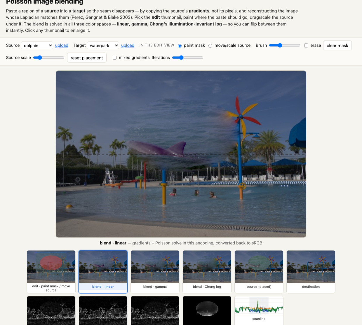
Every choice this chapter has made — which space to integrate in (linear, gamma, or log), whether to mix gradients, and what the gradient fields and the reconstruction actually look like — is easiest to feel by doing it. The interactive playground in Figure 5.1.6 lets you paste one photo into another, paint the region, and watch the seam dissolve as you flip those switches.

The healing brush is a covariant derivative🔗⧉

Photoshop's healing brush — the tool retouchers use to erase a blemish or a stray wire by sampling clean skin or sky nearby — is gradient-domain cloning with a twist, and it came first: Photoshop 7 shipped the healing brush in 2002, before Pérez's paper (2003), which was inspired by it and gave it the clean gradient-domain formulation we have been using. Todor Georgiev (Adobe, 2004/05) later supplied the brush's own theory. The difference is that the healing brush is multiplicative rather than additive. Instead of transporting differences (subtractive gradients), it transports ratios, which it does by working on $\log f$ — exactly the log-domain move we just justified — so that a patched region matches the destination's illumination rather than its absolute brightness. In Georgiev's framing this is a covariant derivative: the gradient is transported in a way that respects the multiplicative structure of lighting. The healing brush is therefore the same linear-versus-log choice we made above, baked permanently into the operator. (Georgiev reaches it through the covariant-derivative machinery of general relativity, which is elegant but notoriously heavy going; working in the log domain gets you essentially the same result far more simply.)

Conservative-gradient simplification: the membrane shortcut🔗⧉

The general Poisson solve is iterative and not cheap, which is what kept early gradient-domain editing off the interactive path. But recall the sidebar: when the guidance field is conservative — when it is the exact gradient of some image $g$, as in a plain clone — the problem simplifies dramatically. We saw the reason already, in the boundary-discrepancy picture: pasting $\nabla g$ and solving Poisson gives exactly the same answer as adding a correction surface to the naive paste, where that correction surface is the smooth membrane that interpolates the boundary mismatch $f^{*}-g$ into the interior. And the membrane solves the much cheaper Laplace equation,

after which the result is simply $g + u$ inside the region. The payoff (Sylvain Paris; Farbman et al. 2009; surveyed in Bhat et al. 2010) is real: a Laplace solve with smooth boundary data is far easier than a full Poisson solve — it can be approximated very fast, even by a coarse mesh or a handful of interpolation steps — and it is the route to real-time gradient-domain editing. The lesson is to recognize the special case: a true-gradient guidance field never needed the heavy machinery; it only ever needed a membrane.

Other gradient-domain edits🔗⧉

Once you see editing as change the guidance field, reuse the solver, the family keeps growing, and several of these get their own treatment later in the book:

• HDR tone compression (Fattal, Lischinski and Werman 2002): a high-dynamic-range scene has a few enormous gradients (the window, the lamp) swamping the rest. Attenuate the large gradients — leave small ones alone, shrink big ones — then integrate the modified field. The huge range collapses while local contrast survives, because we manipulated the gradients and let the absolute level fall out of the solve. Integrate in log, where attenuation is well-behaved.
• Photomontage (Agarwala et al. 2004): stitch many photographs into one by choosing, per region, which source contributes its gradients, then solving Poisson over the whole composite. This is the explicit meeting point of the three legs of this part: a graph-cut seam (the seam-optimization chapter) decides where to switch between sources, and a gradient-domain blend (this chapter) hides whatever residual mismatch the seam leaves — cut along the edges, then reconstruct across them.
• And further afield, all built the same way: shadow and reflection removal (zero out the gradients that belong to the shadow edge, re-integrate) and flash / no-flash fusion (borrow gradients from the sharp flash image while keeping the ambient color). Every one of them changes only $\mathbf{v}$ and reuses the same sparse solver.