2.8 Human (and animal) vision and color🔗⧉

2.8.1 Visual system anatomy:🔗⧉

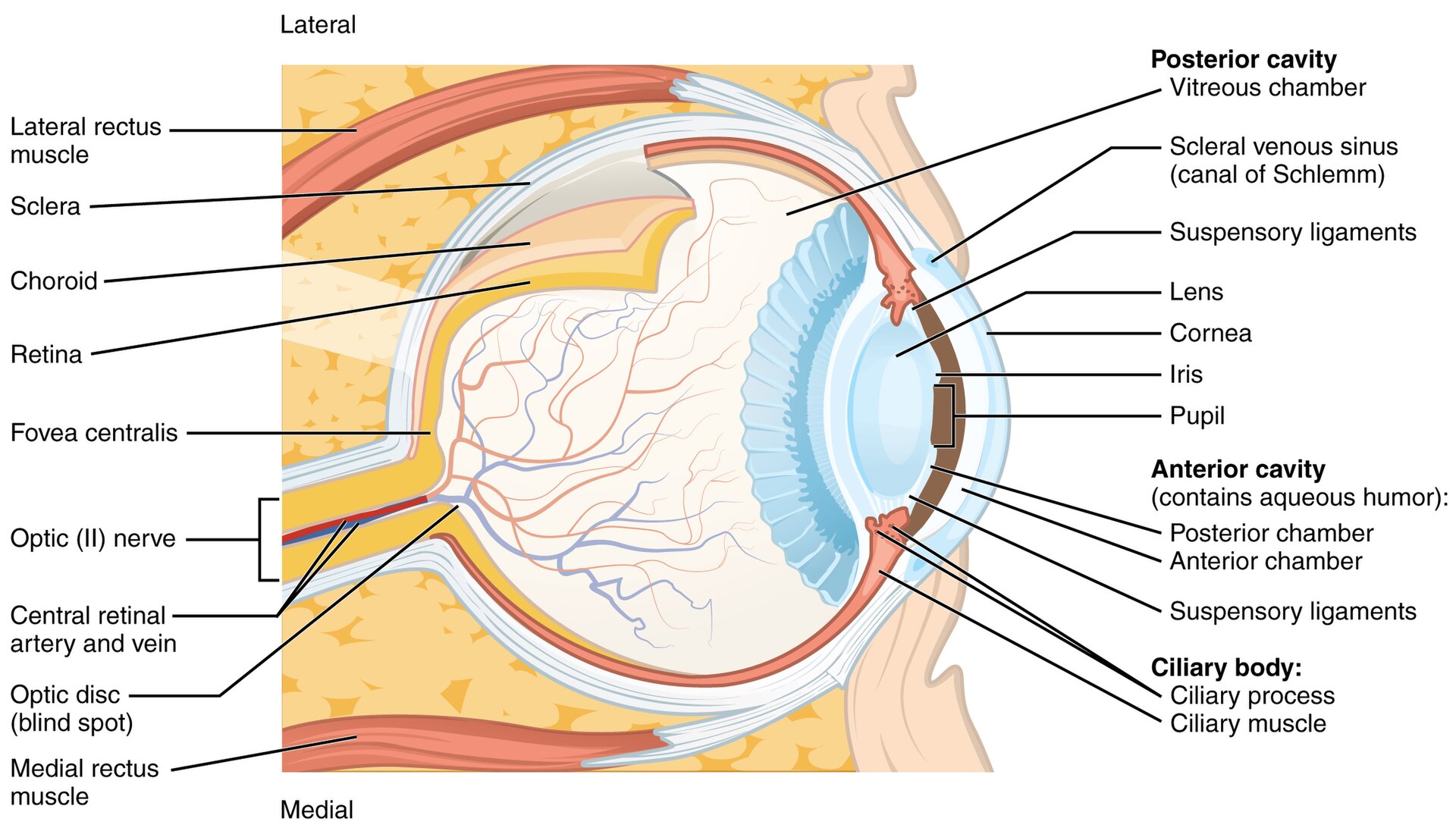
Light entering the eye passes through the cornea and the lens — together the eye's two refracting elements, the same Snell's-law optics as a camera lens (the cornea does most of the bending; the lens fine-tunes focus by changing shape, accommodation). The pupil, the iris's adjustable opening, is the eye's aperture. The image lands on the retina, a thin sheet of neural tissue lining the back of the eyeball (Figure 2.8.1).

The retina's light-sensitive cells come in two families. Rods are exquisitely sensitive and handle dim, night (scotopic) vision, but there is only one kind, so rod vision is colorless. Cones are less sensitive, work in daylight (photopic vision), and come in three types — the basis of color. Their distribution across the retina is wildly non-uniform (Figure 2.8.2). Cones are packed densely in the fovea, the tiny central pit we point at whatever we are scrutinizing; rods dominate the periphery. This is why you cannot read text out of the corner of your eye, and why faint stars are easier to see slightly off-centre.

Two quirks of this layout matter for imaging. First, there are essentially no short-wavelength (S, "blue") cones in the very centre of the fovea, and far fewer S cones than long- and medium-wavelength (L and M) cones overall. As a result blue is sensed at low resolution and is even slightly out of focus — the eye's chromatic aberration puts blue at a different focal plane — yet we perceive a crisp blue everywhere, because the brain fills it in. Second, luminance (our sense of brightness) is roughly the sum of the L and M cone responses, so green carries most of our spatial acuity. This single fact echoes through the whole book: it is why camera color-filter mosaics (the Bayer pattern) use twice as many green cells as red or blue, and why image compression can throw away color detail but not brightness detail.

The retina is not a passive film: it does substantial processing before anything leaves the eye. Photoreceptors feed a network of intermediate cells whose output drives the ganglion cells, whose axons form the optic nerve. Already at this stage the signal is reorganized into centre–surround receptive fields (the seed of lateral inhibition and edge enhancement, returned to under Spatial vision). From the eye the pathway runs to the lateral geniculate nucleus (LGN) of the thalamus and on to the primary visual cortex (V1) at the back of the head, then to higher areas that handle motion, form, and recognition. The lesson for us: much of what we naïvely attribute to "the image" is really a construction, assembled in stages from a heavily pre-processed retinal signal.

2.8.2 Color🔗⧉

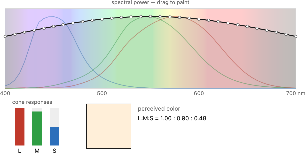
Here is the crux. A cone does not measure wavelength — it produces one number. A given cone type $k$ has a spectral sensitivity $c_k(\lambda)$: a curve saying how strongly it responds to light of each wavelength (Figure 2.8.3). When light with spectrum $E(\lambda)$ arrives, the cone reports a single response, the spectrum weighted by its sensitivity and summed over all wavelengths:

This is a projection — exactly the pixel-as-integral idea from Image formation, now with three spectral filters instead of one. Three cone types give three numbers $(r_L, r_M, r_S)$, and that triple is all the information the eye keeps about the spectrum. An infinity of wavelengths collapses to three.

It helps to make the projection concrete as linear algebra. Discretize the spectrum into $N$ wavelength bins and stack the samples into a vector $\mathbf{E} \in \mathbb{R}^N$. Stack the three sensitivity curves as the rows of a $3 \times N$ matrix $\mathbf{C}$, one row per cone type. Then the three cone responses are just a matrix–vector product,

(Figure 2.8.4). In reality wavelength is continuous, so $N \to \infty$ and the sum becomes the integral above — color sensing is genuinely an infinite-dimensional input squeezed through a three-dimensional bottleneck.

Two consequences follow immediately. The first is that a single cone cannot distinguish wavelengths. Feed it a dim light at its peak wavelength or a brighter light at a wavelength where it responds half as strongly, and it reports the same number — a cone confounds color with intensity. Only by comparing the three cones' outputs can the brain begin to separate the two. This is the principle of univariance, and it is why a pure monochromatic laser line and a carefully chosen mixture of other wavelengths can look identical.

That identity is metamerism, the most important practical fact about color (Figure 2.8.6). Because the map $\mathbf{E} \mapsto \mathbf{r}$ is a projection from infinite dimensions to three, it has an enormous null space: vastly many different spectra produce the same triple $(r_L, r_M, r_S)$ and therefore look exactly the same. Two such spectra are metamers. Metamerism is not a defect — it is what makes color reproduction possible at all. A screen with only three primaries can match (almost) any real spectrum, not by reproducing it, but by producing a metamer of it. The whole edifice of color technology in the next chapter rests on this.

Now the part that makes the linear algebra messy, and the reason for the lesson placed here. The three cone "axes" are not orthogonal — look again at Figure 2.8.3, where L and M overlap almost completely. And spectra, being physical power densities, cannot be negative, so the cone responses live only in the positive octant. Both facts conspire against the comfortable picture of an orthonormal basis where analysis equals synthesis.

To unpack the figure: synthesis — building a color from the basis — is the easy direction; any point is a weighted sum of the two cone vectors, and because they both sit in the positive quadrant we can always do it with non-negative weights. Analysis — recovering the weights $a_1, a_2$ that produced a given color — is the hard direction. It is not the perpendicular projection onto $c_1$ and $c_2$ that orthonormal intuition suggests. The correct operation is to project onto the dual basis $c_1^{*}, c_2^{*}$, the vectors defined by $c_i^{*}\!\cdot c_j = \delta_{ij}$. For a non-orthogonal positive basis those dual vectors necessarily reach into the negative quadrants — they have negative coordinates in the original space. That is the precise sense in which "stuff can't be negative" makes color hard: the natural analysis vectors are exactly the ones light cannot realize. (Only when the basis is orthonormal do a basis and its dual coincide, and analysis collapses back into simple projection.)

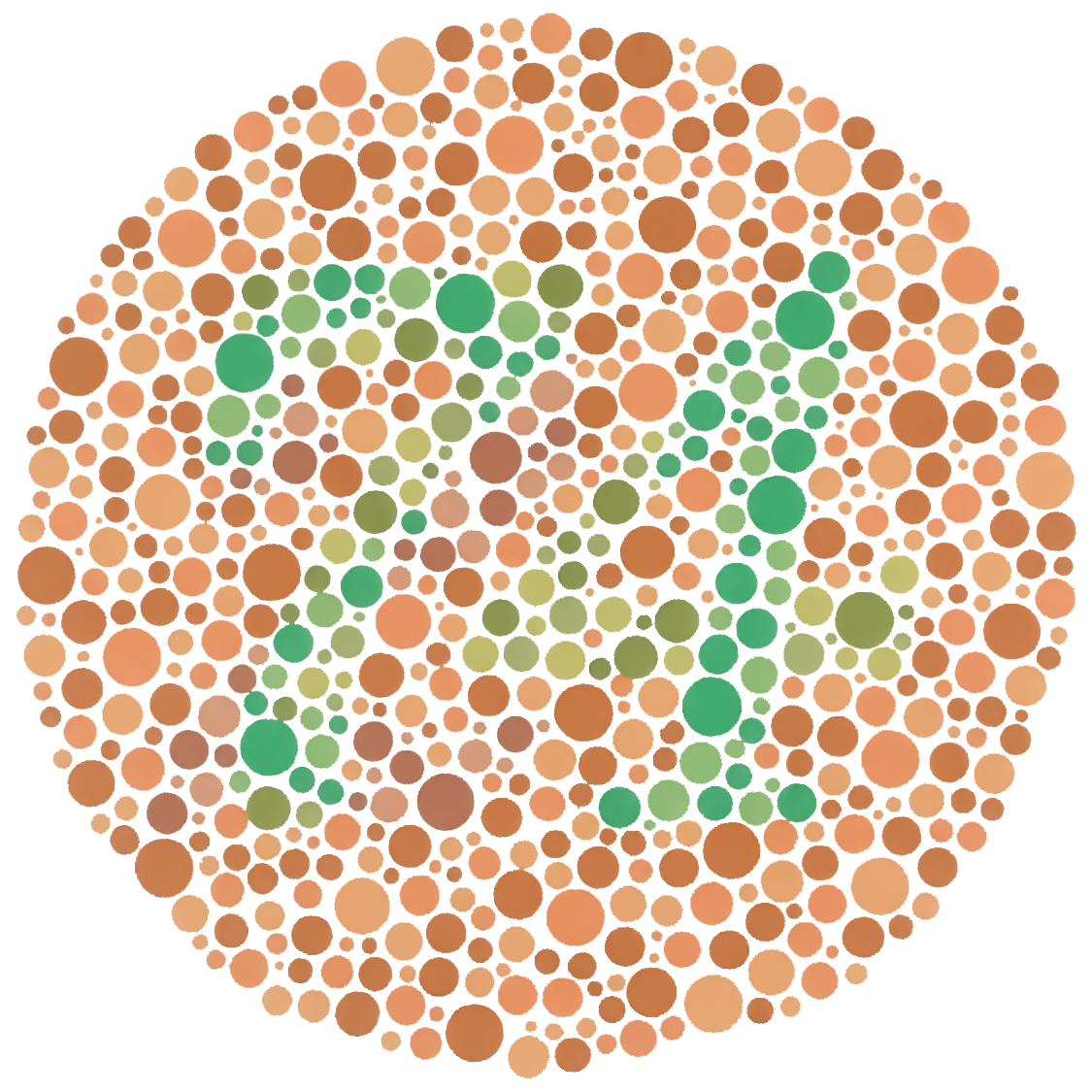
Color blindness is what happens when this projection loses even more information. A "dichromat" is missing one cone type (most commonly through the L/M genes), so the spectrum is projected onto two numbers instead of three; many spectra that look distinct to a trichromat now collapse into the same response — the classic red–green confusion. The standard Ishihara plates (Figure 2.8.8) exploit exactly this, hiding a figure that a trichromat sees and a dichromat cannot. The deeper point is one of perspective: a trichromat is also projecting away an infinity of spectral information. We are all color-blind relative to the full spectrum — and, as the next sidebar shows, relative to other animals too.

Finally, the brain does not stop at three cone numbers. It re-codes color through a multistage model (simplified here; the full version is in Reinhard et al., Color Imaging):

• Stage 1 — cones. Three heavily overlapping L/M/S responses, the projection above.
• Stage 2 — opponent recoding, in the retina and the lateral geniculate nucleus. The L/M/S signals are re-mixed into three opponent channels: light–dark, red–green, and blue–yellow. This decorrelates the channels (since L and M are so redundant, their difference carries the color information efficiently) and matches the four "unique hues" we feel — the subject of the next section.
• Stage 3 — appearance. A higher-level organization closer to hue, saturation, and brightness (a hue-saturation-value-like, or HSV-like, arrangement), where context, adaptation, and memory shape the final percept — the domain of color-appearance models in the next chapter.

The recoding is not arbitrary. Color names cluster around shared focal colors across unrelated languages (Berlin & Kay's classic study, and the broader World Color Survey) — evidence that the structure is perceptual, built into the wiring rather than the culture. The recoding has support from two directions: psychophysics (Hurvich and Jameson's hue-cancellation experiments) and physiology (De Valois's recordings of opponent cells).

2.8.3 So what are the primary colors?🔗⧉

Everyone has argued about this. Is it red-green-blue (RGB)? The grade-school red-yellow-blue (RYB)? Cyan-magenta-yellow (CMY)? The perennial muddle has two separate causes, and — this is the key insight — neither of them is a fact about light.

The first cause is the opponent recoding we just met. Because the visual system re-wires the three cone signals into red–green, blue–yellow, and light–dark, red, green, blue, and yellow all feel "primary" to us perceptually — there are four psychological unique hues, not three. This is why red-yellow-blue feels so natural to painters, and why the cones' actual L/M/S sensitivities match nobody's intuition of "primary" colors: our intuition is reporting the opponent stage, not the cones.

The second cause is additive versus subtractive synthesis, a matter of technology (taken up fully in the next chapter). RGB are the additive primaries — the colors of light you add together on a screen. CMY are the subtractive primaries — the inks or filters that remove light from white. The grade-school RYB is just a folk approximation of subtractive mixing.

So "primary color" silently conflates a perception fact with a technology choice — two different questions with two different answers, neither of which is intrinsic to the physics of light. As the lecture put it, the opponent rewiring "is one of the many causes of all the confusion about what's a primary color." (See the Glossary entry for primary.)

2.8.4 Opponent process and the multistage model🔗⧉

The two-stage story is worth stating cleanly: color is trichromatic at the cones, then opponent in the retina and lateral geniculate nucleus. The three cone signals are recombined into three opponent channels — red–green (roughly $L - M$), blue–yellow (roughly $S - (L+M)$), and light–dark (roughly $L + M$, the luminance channel). In symbols this is just a fixed linear map,

with $\mathbf{M}$ a $3 \times 3$ matrix — the perceptual ancestor of the luma–chroma transforms (the $Y'C_bC_r$ of JPEG) we will use later (Figure 2.8.10).

This model earns its keep in two ways. It explains afterimages: stare at a saturated red patch until the red–green channel adapts, then look at white and the channel rebounds the other way, painting a green ghost (likewise blue→yellow). And it explains why luma/chroma encodings compress so well: the luminance channel ($Y'$, computed on gamma-encoded RGB — see Linear vs Gamma next chapter) carries most of the detail we can resolve, while the two chroma channels can be heavily subsampled with little visible loss — the foundation of JPEG's chroma subsampling, and a direct prediction of the opponent model that we will confirm under Spatial vision.

2.8.5 Light adaptation🔗⧉

The eye faces a dynamic range that no single setting could span — starlight to direct sun is a factor of billions. It copes not by capturing it all at once but by adapting over time, continually recentering its response around the current average brightness. Walk into a dark cinema and you are blind for a minute, then the seats swim into view; step back out and the lobby is blinding before it settles. The neural response to intensity $I$ is well described by a saturating (Naka–Rushton) curve,

an S-shaped function whose half-saturation point $I_0$ slides to track the prevailing light — so the limited response range is always spent where it is useful.

Three mechanisms cooperate across different timescales: neural gain control (fast), photochemical bleaching and regeneration of the photopigment (slower — the minutes of dark adaptation), and the pupil (a quick but small contribution, a couple of stops at most). The consequences are everywhere: afterimages again (a local adaptation that leaves a stamp when the gaze moves), and striking illusions of motion such as the Spanish-Castle illusion, where staring at a color-reversed image and then a blank field produces a fleeting full-color positive — adaptation of the opponent channels writ large (Figure 2.8.11). Adaptation is why the eye's "dynamic range" is so often overstated: it is huge over time, far smaller in any single instant — exactly the gap that high-dynamic-range (HDR) capture and tone mapping (later chapters) must bridge.

Where the eye operates also changes which receptors do the work, and we name three regimes by the prevailing luminance (in candela per square metre, $\text{cd/m}^2$ — the photometric "nit" from Light and physics, light measured along a ray). They are (Figure 2.8.12):

• Photopic (daylight): the cones are in charge, giving full color and sharp foveal vision. Roughly above $3\,\text{cd/m}^2$ — office light sits near $10^{2}$, an overcast sky around $10^{3}$–$10^{4}$, a sunlit scene around $10^{4}$–$10^{5}\,\text{cd/m}^2$.
• Mesopic (dusk or a dim interior): rods and cones work together, roughly $10^{-3}$ to $3\,\text{cd/m}^2$. Colors desaturate and the Purkinje shift sets in — as rods take over, blues look relatively brighter and reds relatively darker (the flowers that glowed red at noon go murky at dusk while the blue foliage stays luminous).
• Scotopic (night): rods only — no color, poor acuity, and notably off-fovea, since the all-cone fovea is effectively blind in the dark (which is why a faint star vanishes when you look straight at it). Below about $10^{-3}\,\text{cd/m}^2$ — a moonlit landscape near $10^{-2}$, starlight around $10^{-3}$–$10^{-4}$, and the absolute threshold of vision down near $10^{-6}\,\text{cd/m}^2$ (a handful of photons).

The big picture is staggering: across these regimes the eye works over roughly $10^{-6}$ to $10^{8}\,\text{cd/m}^2$ — about 14 log units of luminance — yet it spans only a few log units at any one instant. That gap between the total range and the instantaneous range is precisely why adaptation exists in the eye, and precisely why cameras need high-dynamic-range (HDR) capture and tone mapping (later chapters) to pack a scene's range into a display's.

2.8.6 Lightness constancy🔗⧉

Adaptation handles the overall level. A subtler and more impressive feat handles spatial structure: the visual system reports a surface's intrinsic lightness — its reflectance, the fraction of light it bounces back — and not the raw luminance reaching the eye. A white page carried into shadow still looks white; a lump of coal in sunlight still looks black — even when the shadowed page sends less light to your eye than the sunlit coal. The brain is reporting the property of the surface, not the photons.

To do this it must discount the illuminant. Recall from Light and physics that the light reaching the eye is illumination × reflectance — the same multiplicative entanglement as everywhere in imaging. The brain factors that product and reports the reflectance alone, because reflectance is the thing we actually care about (what is this object?). But this is an ill-posed inversion: one measured image, two unknowns (light and surface) at every point. The brain solves it with cues and priors — chiefly edges and context, reading sharp edges as changes in the surface and slow gradients as changes in the illumination.

The canonical demonstration is Adelson's checker-shadow illusion (Figure 2.8.13): two checkerboard squares of identical pixel luminance look dramatically different — one "white in shadow," one "black in light" — because the brain infers the cast shadow and discounts it. Retinex (Land & McCann 1971) models exactly this computation: treat slow spatial gradients as illumination and sharp edges as reflectance changes, then integrate the edges back up to recover lightness. The same idea reappears as intrinsic images (splitting a photo into a reflectance layer and a shading layer) and, in the darkroom, as the craft of dodging and burning — locally cheating the illuminant that the eye is trying so hard to discount.

2.8.7 Color constancy🔗⧉

Color constancy is the chromatic twin of lightness constancy. We perceive an object's intrinsic surface color — its spectral reflectance — despite large swings in the illuminant. A white shirt reads as white under noon daylight, under a warm tungsten lamp, and in cool blue shade, even though the spectra reaching the eye in those three cases differ enormously. Once again the brain discounts the illuminant: it estimates the color of the light and effectively divides it out, so the surface reads consistently. And once again this is the illuminant × reflectance inversion — ill-posed, solved with assumptions, such as "the average of the whole scene is roughly grey" or "the brightest patch is white."

A key biological mechanism is von Kries adaptation: an independent gain on each cone type (L, M, S) that rescales each channel to the prevailing light (Figure 2.8.14). It is beautifully simple — three multipliers — and it is the direct biological ancestor of a camera's white balance. It is also not perfect: some cast lingers, spatial and contextual cues fill the rest, and memory colors (we know bananas are yellow and grass is green) bias the result.

This whole process is the biological counterpart of white balance (next chapter): the camera's automatic white balance algorithm must compute, by gray-world, bright-pixel, Retinex, or Bayesian (Freeman & Brainard) heuristics, what our visual system does for free. And because the inference is genuinely ambiguous, different observers can resolve it differently — which is the whole story of "the dress" (Figure 2.8.15). The viral 2015 photograph shows identical pixels that some people see as blue-and-black and others as white-and-gold, because each viewer's brain silently guesses the illuminant — cool daylight versus warm indoor light — and divides it out differently. The dress is the perfect proof that color constancy is an inference under uncertainty, not a measurement: the visual system commits to a prior, and different people commit to different priors. A camera faces the exact same ill-posed guess.

2.8.8 Contrast🔗⧉

If there is one mathematical theme to perception, it is that vision cares about ratios, not absolute values — a direct consequence of operating in a multiplicative world under wildly varying light. A step from luminance 1 to 2 looks like the same step as 100 to 200: in both cases the light doubled, and doubling is what the eye registers. This automatically discounts the multiplicative effect of the illuminant (a brighter light scales everything equally, leaving ratios untouched) and it is the direct perceptual reason we will later encode images in gamma or log — to spend code values where the eye actually looks.

Quantitatively, this is Weber's law: the just-noticeable increment in intensity is roughly a constant fraction of the background, $\Delta I / I \approx \text{const}$. The smallest brightness change you can detect grows in proportion to the brightness you are already looking at — the signature of a logarithmic-ish response. For describing the contrast of a pattern (rather than a single increment) the standard measure is Michelson contrast,

a normalized, level-independent ratio. Contrast also depends on context: a grey patch looks lighter on a dark surround and darker on a light one (simultaneous contrast), and the Adelson checker-shadow illusion is the same effect dressed up. Ratios, not absolutes, all the way down.

2.8.9 Spatial vision🔗⧉

How fine a pattern can we resolve, and how does sensitivity vary with the scale of the detail? Visual acuity — the familiar eye-chart measure — sets the finest line spacing we can make out, but it is only the high-frequency tail of a richer story.

Two low-level mechanisms shape spatial vision. Lateral inhibition wires each retinal cell to subtract a weighted average of its neighbours, producing centre–surround receptive fields that respond to local contrast rather than absolute level — an edge enhancer built into the retina. Its signature is Mach bands (Figure 2.8.16): at a ramp between two grey levels you see illusory bright and dark bands hugging the edges, the centre–surround filter overshooting. The same wiring underlies simultaneous contrast from the previous section.

The full description is the contrast sensitivity function (CSF), measured by psychophysics: show the observer sine-wave gratings of varying spatial frequency and contrast, ask "do you see a grating?", and trace the threshold. The CSF turns out to be band-pass — sensitivity peaks at intermediate spatial frequencies and falls off at both very coarse and very fine scales (the high-frequency cutoff is acuity). Crucially, there is not one CSF but three, and they differ dramatically (Figure 2.8.17): the chromatic CSFs — for the red–green and blue–yellow opponent channels — cut off at far lower spatial frequency than the luminance CSF. We resolve color far more coarsely than brightness.

This yields one of the most consequential demonstrations in the book. Convert an image to an opponent (luma/chroma) space and blur the chroma channels heavily — the picture still looks sharp. Blur the luminance channel instead and it falls apart. The eye simply does not resolve fine color. This is the empirical licence for chroma subsampling in JPEG and video (store color at half or quarter resolution), and a clean confirmation of the opponent model and its three separate CSFs.

2.8.10 Temporal vision🔗⧉

The visual system trades some spatial resolution for temporal resolution. Just as there is a contrast sensitivity function over spatial frequency, there is a temporal CSF over flicker frequency, and it too is band-pass. Above a critical flicker-fusion frequency — roughly 50–60 Hz in bright light, lower in dim — a flickering source fuses into a steady one. This is why displays and projectors refresh fast enough to look continuous, and why old cathode-ray-tube screens and fluorescent tubes could be seen to flicker in peripheral vision (the periphery, rod-rich, has a higher fusion frequency) even when the centre of gaze saw them as steady.

Closely related is apparent motion — the phi phenomenon — by which a sequence of still frames reads as continuous movement; together with persistence of vision it is what makes cinema and video possible (→ Motion/Video). Temporal vision also has its own adaptation (the seconds-to-minutes light/dark adaptation of the previous section) and is shaped by the eye's own constant motion — the saccades and microsaccades of the next section. Computation exploits all of this: choosing frame rates, capturing flicker-free under pulsed lighting, and video magnification (amplifying tiny, normally invisible temporal changes — a color or motion signal too small to notice — covered in Motion/Video).

2.8.11 Attention and eye movements🔗⧉

Vision is not a uniform snapshot. Only the fovea sees in high resolution, so the eye samples a scene through a rapid sequence of fixations punctuated by saccades — fast, ballistic jumps that re-aim the fovea — with smooth pursuit to track moving targets. We feel as though the whole scene is sharp, but that is another construction: the brain stitches together a few high-resolution glimpses and fills in the rest. A record of where the eye lands over time is a scanpath (Figure 2.8.18), and it is far from random — it is drawn to salient regions (faces, motion, high contrast, the unexpected).

What draws the eye — saliency — can be modelled, and modern saliency and gaze-prediction models are learned with machine learning (→ the saliency / gaze-prediction material in the Machine learning part). Saliency in turn feeds content-aware image operations: where can we crop or retarget an image without disturbing what the viewer will actually look at? That is the link to auto-cropping and seam carving later in the book.

2.8.12 Perception of color and images🔗⧉

A last cluster of phenomena matters specifically for reproducing images, where the goal is for a print or screen to look like the original even though the physical stimulus differs. Several perceptual effects mean that "matching the numbers" is not enough.

Color appearance shifts with viewing conditions. There is a general blue shift in dim light and a tendency for the perceived white point to drift. Colorfulness grows with luminance — the Hunt effect: the same surface looks more vividly colored when brightly lit than when dim, which is why images viewed on a bright display or in a bright room read as more saturated (Figure 2.8.19). And hue itself shifts with two independent variables: with intensity (the Bezold–Brücke shift, where a color's hue changes as it is made brighter or dimmer) and with added white (the Abney effect, where desaturating a color shifts its apparent hue).

These appearance phenomena — together with adaptation and constancy — are why faithful color reproduction needs color-appearance models that account for the viewing environment (Fairchild, Color Appearance Models), and they are part of why artists exploit perceptual quirks so effectively (Livingstone, Vision and Art). They set up the next chapter's engineering: now that we know how the eye sees color, we can build the technology to measure, encode, and reproduce it.

2.8.13 Animal eyes🔗⧉

Human vision is one solution among many, and a parochial one. Eyes have evolved independently dozens of times, and surveying the alternatives is the best cure for treating our own visual system as the definition of "seeing." Two questions organize the tour, the same two that organize the whole book's treatment of a camera: how is the image formed (optics), and how is color sensed (the photoreceptors and their wiring). The optical side connects back to Image formation; the color side extends the opsin story above.

The optics: many ways to form an image🔗⧉

Forming an image means getting light from each direction in the scene onto a different receptor — the same plenoptic-sampling problem a camera solves with a lens. Nature has found several radically different answers (Figure 2.8.21).

Before the variety, the sequence. A full eye is not an all-or-nothing leap but a ladder of small, individually useful improvements (Land & Nilsson). Start with a flat patch of photoreceptors that registers only light versus dark; fold it into a cup, and the rim shades part of the sheet, giving a crude sense of direction; close the cup to a pinhole, and a real (if dim) inverted image forms with no lens at all; finally fill the aperture with a lens for a bright, focused image. That progression — from no image to a focused one — recapitulates the optics of this book in miniature (Figure 2.8.20).

• Single-lens ("camera") eyes, like ours and the octopus's, use one refracting element to cast a single inverted image on a sheet of receptors — the design we have been modelling all chapter. The vertebrate and cephalopod versions evolved separately and even wire their retinas back-to-front relative to each other, a textbook case of convergent evolution onto the same optics.
• Compound eyes (insects, crustaceans) tile the visual field with hundreds or thousands of ommatidia, each a tiny lens feeding one or a few receptors and pointing in a slightly different direction. Resolution is set by how finely the facets are packed, not by a single aperture — so acuity is modest, but the field of view is enormous and the temporal response very fast (one reason flies are so hard to swat). It is, in effect, a fixed array of one-pixel cameras.
• Lens-less designs solve image formation without refraction at all: the pinhole eye of the nautilus (an aperture with no lens — sharp but dim, exactly the pinhole-camera tradeoff from Image formation), and the mirror ("reflecting") eyes of scallops and some deep-sea crustaceans, which focus by a curved multilayer mirror behind the retina rather than a lens — the biological analogue of a catadioptric camera.
• Eyes built for a niche. Many designs are tuned to a task more than to general acuity: the tapetum lucidum, a reflective layer behind the retina in cats, dogs, and deer, bounces unabsorbed photons back through the receptors for a second chance — boosting night sensitivity at the cost of a little blur (and causing eyeshine in a flash photo). Deep-sea fish stack receptors or grow tubular eyes to wring signal from a few photons; the four-eyed fish Anableps splits its cornea to focus above and below the waterline at once.

The color vision: opsins remixed🔗⧉

If the optics vary, color vision varies even more, because "color" is nothing but whichever set of opsins (the light-sensitive photopigment proteins) an animal happens to carry — and, crucially, how it compares their outputs. Three lessons stand out, all of them sharpening points made earlier in the chapter.

• More dimensions than three. Our trichromacy is not a ceiling. Many birds, reptiles, and fish are tetrachromats, with a fourth cone reaching into the ultraviolet (UV) — they see patterns on flowers and plumage that are simply invisible to us. Most mammals, by contrast, are dichromats (red–green "color-blind" by our standard); primate trichromacy is re-evolved, the product of a recent gene duplication that split one pigment into our overlapping L and M cones — which is exactly why L and M overlap so heavily (the opsin sidebar above). The lesson from the metamerism section returns with teeth: every species is "color-blind" relative to some other, ourselves included, because every visual system projects an infinite spectrum onto a handful of numbers.
• More receptors do not mean more discrimination. The mantis shrimp carries roughly twelve to sixteen photoreceptor classes — and yet discriminates colors rather poorly in behavioural tests. The leading interpretation is that it does not compare channels the way a trichromat does (the comparison that the univariance section showed is essential); instead it appears to recognize colors almost directly, reading off which receptor fires hardest. It is a working counterexample to "more channels = better color," and a reminder that color lives in the wiring, not just the pigments.
• Sampling axes we lack entirely. Some animals sense components of the plenoptic function we cannot. Many insects and cephalopods are sensitive to the polarization of light, using it to navigate by the sky's polarization pattern or to cut glare off water (recall polarization from Light and physics) — the mantis shrimp even senses circular polarization. Others extend their spectral window well outside our 400–700 nm band: pit vipers image thermal infrared with a separate pit organ, and UV-sensitive species push the short-wavelength end. Each species samples a different slice of the same physical world.

The opsin family tree and the divergence behind all this are traced in the "Evolution of Eyes" chapter of Vision (Cambridge) Vision, "Evolution of Eyes"; the schematic gene tree is Figure 2.8.9 above.

The throughline of the whole chapter — now stated across species: color and vision are not read off the world, they are computed from it — projected through whatever opsins an eye carries, re-coded by whatever wiring sits behind them, adapted, and inferred. Human vision is one particular such computation; every later chapter on color, encoding, and image quality is an attempt to live within, or exploit, the constraints our version of that biological processor imposes.