22.9 Problem Set 7 — Automatic panoramas🔗⧉

22.9.1 Summary🔗⧉

• Class morph
• Harris corner detection
• Patch descriptor
• Correspondences using nearest neighbors (NN) and the second NN test
• RANSAC
• Fully automatic panorama stitching of two images
• Linear blending
• Two-scale blending
• Mini Planets
• 6.8370: N-image Panoramas
• Make your own panorama!

This is not an easy assignment, but you have two weeks to complete it. Make sure you start early!

There are many steps that all depend on the previous ones and it's not always trivial to debug intermediate results. We provided you with visualization helpers which you can read about throughout this pdf or in panorama.cpp.

22.9.2 Previous Problem Set Code🔗⧉

This Problem Set uses code from Problem Set 6. Replace the functions in homography.cpp with your own code (you can copy the entire file).

22.9.3 Class Morph🔗⧉

We have put the photos for your class morph on Piazza.

Search for your username you used to log into the submission website for your photograph, and use the morph program you wrote for problem set 5 to morph to the next person on the list. Draw the segment pairs until the result looks good enough (you would probably need at least 8). Please generate 30 frames (excluding the source and target frame).

• Q. Generate your morphing images and put them in a class_morph folder in your submission (inside your asst folder.) Name your images class_morph_%02d.png (where %02d is replaced by the frame number, e.g. class_morph_01, class_morph_02, ...). Notice that you should have 32 images, numbered from 0 to 31, including the source and target photos. Please also write a file called segments.txt, containing the C++ code of the segments you used to perform the morphing, generated from the javascript UI.

We will compile everyone's images and make a video of every person morphing to every other person in the class.

22.9.4 Harris Corner Detection🔗⧉

The Harris corner detector is founded on solid mathematical principles, but its implementation looks like following a long cookbook recipe. Make sure you get a good sense of where you're going and debug/check intermediate values.

Structure tensor🔗⧉

The Harris Corner detector is based on the structure tensor, which characterizes local image variations. We will focus on greyscale corners and forget color variations.

We start from the gradient of the luminance $I_x$ and $I_y$ along the $x$ and $y$ directions (where subscripts denote derivatives). The structure tensor at pixel $(i,j)$ is:

Notice that $M$ is a $2 \times 2$ symmetric matrix so we can only store the 3 unique entries.

In order to compute $M$, we first extract the luminance of the image using the lumiChromi function from Pset 1. Using a Gaussian with standard deviation sigmaG, blur the luminance to control the scale at which corners are extracted. A little bit of blur helps smooth things out and help extract stable mid-scale corners. More advanced feature extraction uses different scales to add invariance to image scaling.

Next, compute the luminance gradient along the x and y direction. We've added the functions gradientX and gradientY in filtering.cpp for you. Call these functions with the default value of clamp.

At this point we have the per-pixel $I_x$ and $I_y$ components needed for the computation of the tensor equation. We will represent the tensor as an image the same size as the input image, where the channels correspond to the 3 unique entries of the tensor, e.g. the channels correspond to $I_x I_x$, $I_x I_y$, $I_y I_y$.

To complete the computation of the tensor, we weight each of the gradient components of the tensor equation by a weighting function. The final tensor is:

where we skipped the pixel index for clarity. The weighting function does a local weighted sum of the tensors at each pixel in order to take into account the values of the neighbors. In our case, the weighting function is a Gaussian. To achieve this last step, simply call the function gaussianBlur_separable with the tensor computed above and standard deviation sigmaG*factorSigma (and the default truncation value).

• Q. Write a function Image computeTensor(const Image &im, float sigmaG=1, float factorSigma=4) in panorama.cpp that returns a 3D array (i.e. an Image) of the size of the input where the three channels at each location x, y store the three values corresponding to the $I_xI_x$, $I_xI_y$, and $I_yI_y$ components of the final tensor (in this order). Hint: don't forget to blur as specified above.

Harris corners🔗⧉

Implementing the Harris corner detectors require a few steps, presented here in order. Read the whole subsection before starting your implementation.

Corner response. To extract the Harris corners from an image, we need to measure the corner response from the structure tensor. The measure of corner response is $R=det(M)-k(trace(M))^2$, which compares whether the matrix has two strong eigenvalues, indicative of strong variation in all directions (see class notes).

• Q. Implement Image cornerResponse(const Image &im, float k=0.15, float sigmaG=1, float factorSigma=4) in panorama.cpp that computes the structure tensor of input image im by calling computeTensor and returns a one-channel image the size of im containing the per-pixel corner response.

Non-maximum suppression. We get a strong corner response in a the neighborhood of each corner. We need to only keep the strongest response in this neighborhood. For this, we need to reject all pixels that are not a maximum in a window of maxiDiam. We've written a function maximum_filter in filtering.cpp that you might find useful - be sure to read and understand it fully before incorporating.

Removing boundary corners. Because we will eventually need to extract a local patch around each corner, we can't use corners that are too close to the boundary of the image. Exclude all corners that are less than boundarySize pixels away from any of the four image edges.

Putting it all together. You are now ready to implement HarrisCorners. In the end, your function should return a list of Points containing the coordinates of each corner. For this assignment, we provide a class Point. Each point corresponds to a Harris corner. Note that only pixels with positive corner responses can be corners.

• Q. Implement a function vector<Point> HarrisCorners(const Image &im, float k=0.15, float sigmaG=1, float factor=4, float maxiDiam=7, float boundarySize=5) that returns a vector of 2D Points. Implement the algorithm following the steps outlined above.

More bells and whistles such as adaptive non-maximum suppression or different luminance encoding might help, but this will be good enough for us.

22.9.5 Descriptor and correspondences🔗⧉

Descriptors characterize the local neighborhood of an interest point such as a Harris corner so that we can match it with the same point in different images.

Points in two images are put in correspondence when their descriptors are similar enough. We will call the combination of an interest point's coordinates and its descriptor a Feature, with corresponding class Feature implemented in panorama.cpp.

Our descriptors will be all the pixels in a radiusDescriptor2+1 by radiusDescriptor2+1 window around the associated interest point. That is, they will be a small single-channel Image patch of size $9\times 9$ when radiusDescriptor=4, whose center pixel has the coordinates of the point.

We also want to address potential brightness and contrast variation between images. For this, we subtract the mean of each patch, and divide the resulting patch by its standard deviation. Note that, as a result of the offset and scale, our descriptors will have negative numbers and might be greater than 1. We have added the Image::mean and Image::var methods to simplify the process.

Descriptors🔗⧉

• Q. Write a subroutine Image descriptor(const Image &im, const Point &p, float radiusDescriptor=4) that extracts a single descriptor around interest Point P as described above. Here, im is a single-channel Image (since we will be computing descriptors based on the luminance alone). Hint: don't forget to offset and scale as described above.

Features🔗⧉

As mentioned above, we define a Feature as a pair $(p,d)$ where $p$ is a Point and $d$ is the corresponding Descriptor encoded as a single-channel Image patch. See our Feature class in panorama.h for more information.

• Q. Write a function vector<Feature> computeFeatures(const Image &im, const vector<Point> &cornersL, float sigmaBlurDescriptor=0.5, float radiusDescriptor=4) that takes as input a list cornerL of Harris corners and computes the associated features. The function should return a vector of features the same size as the number of input corners. As noted above, the description will be computed on a single-channel image, to do so, extract the luminance from the input image im, and apply Gaussian blur with standard deviation sigmaBlurDescriptor (this avoids aliasing issues). Compute the descriptions using this blurred luminance.

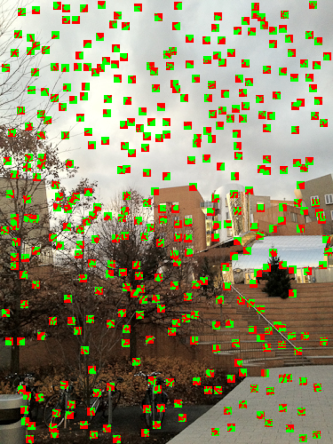
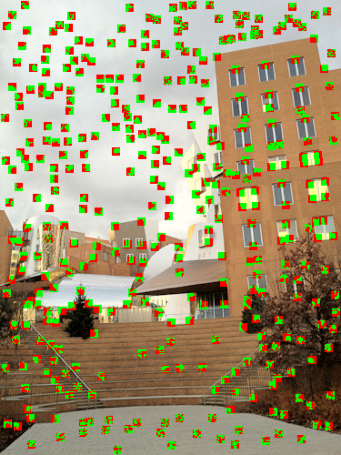
We provided you with a function visualizeFeatures that overlays the descriptors at the location of their interest points, with positive values in green and negative values in red. The normalization by the standard deviation makes low-contrast patches harder to recognize, but high-contrast ones should be easy to debug, e.g. around the tree or other strong corners.

Best match and 2nd best match test🔗⧉

Now that we have code that can compute a list of features for each image, we want to find correspondence from features in one image to those in a second one. We will use our descriptors and the $L_2$ norm to compare pairs of features. The procedure is not symmetric (we match from the first to the second image). We will use the FeatureCorrespondence class, declared in panorama.h.

Let us first implement the Euclidean distance between features:

• Q. Implement float l2Features(const Feature &f1, const Feature &f2) in panorama.cpp that returns the squared distances between the feature descriptors. The squared distance between two descriptors is the sum of squared differences between individual values.

Second-best test. If you remember the discussion in class, for our matching procedure, not only do we consider the most similar descriptor, but also the second best. If the ratio of distances of the second best to the best is less than threshold, we reject the match because it is too ambiguous: the second best match is almost as good as the best one. A word of caution be consistent in your use of distance and squared-distance; you can compute everything with just the squared distance (it's faster, no need for sqrt) but then you need to use the square of the threshold.

• Q. Write a function vector<FeatureCorrespondence> findCorrespondences(const vector<Feature> &listFeatures1, const vector<Feature> &listFeatures2, float threshold) that computes, for each feature in listFeatures1, the best match in listFeatures2, but rejects matches when they fail the second-best comparison. As usual, a helper function could prove useful. The search for the minimum (squared) distance can be brute force.

Your function findCorrespondences should return a vector of FeatureCorrespondence (pairs of 2D points) corresponding to the matching interest points that passed the test. The size of this list should be at most that of listFeatures1, but is typically much smaller.

22.9.6 RANSAC🔗⧉

So far, we've dealt with the tedious engineering of feature matching. Now comes the apotheosis of automatic panorama stitching, the elegant yet brute force RANSAC algorithm (RANdom Sample Consensus). It is a powerful algorithm to fit low-order models in the presence of outliers. Read the whole section and check the slides to make sure you understand the algorithm before starting your implementation. If you have digested its essence, RANSAC is a trivial algorithm to implement. But start on the wrong foot and it might be a path of pain and misery.

In our case, we want to fit a homography that maps the list of feature points from one image to the corresponding ones in a second image, where correspondences are provided by the above findCorrespondences function. Unfortunately, a number of these correspondences might be utterly wrong, and we need to be robust to such so-called outliers. For this, RANSAC uses a probabilistic strategy and tries many possibilities based on a small number of correspondences, hoping that none of them is an outlier. By trying enough, we can increase the probability of getting an attempt that is free of outliers. Success is estimated by counting how many pairs of corresponding points are explained by an attempt. Our RANSAC function will estimate the best homography from a listOfCorrespondences.

Random correspondences. For each RANSAC iteration, pick four random pairs in listOfCorrespondences. The function vector<FeatureCorrespondence> sampleFeatureCorrespondences(vector<FeatureCorrespondence> list) can help you randomly shuffle the vector, and you can then use the first four entries as the four random pairs.

Converting correspondences. Given four pairs of points computed above, you should compute a homography using the functions from problem set 6. In that problem set you used the class CorrespondencePair to specify the pairs of points. We supply you with a function vector<CorrespondencePair> getListOfPairs(const vector<FeatureCorrespondence> &listOfCorrespondences) to convert FeatureCorrespondence to CorrespondencePair, this function expects a list of at least 4 correspondences and returns a vector of CorrespondencePair. To call your computeHomography the method vector<CorrespondencePair>::data() might be helpful.

Singular linear system. In some cases, the four pairs might result in a singular system for the homography. Our first solution was to test the determinant of the system and return the identity matrix when things go wrong. It's not the cleanest solution in general, but RANSAC will have no problem dealing with it and rejecting this homography, so why not? Use the determinant method from Eigen's Matrix class to achieve this.

Scoring the fit. We need to evaluate how good a solution this homography might be. This is done by counting the number of inliers. If the number of inliers of the current homography is greater than the best one so far, keep the homography and update the best number of inliers.

• (a) Implement vector<bool> inliers(Matrix H, const vector<FeatureCorrespondence> &listOfCorrespondences, float epsilon=4). The function should return a list of Booleans of the same length as listOfCorrespondences that indicates whether each correspondence pair is an inlier, i.e., is well modeled by the homography. For this, use the test $||p'-Hp||<$epsilon. Where $p$ is the location of feature 1 and $p'$ is the location of feature 2. That is, the pair $p, p'$ is said to be an inlier with respect to a homography $H$ if $||p'-Hp|| < $epsilon ($||\cdot||$ indicates L2 norm).
• (b) Write a function Matrix RANSAC(const vector<FeatureCorrespondence> & listOfCorrespondences, int Niter=200, float epsilon=4) that takes a list of correspondences and returns a homography that best transforms the first member of each pair into the second one. Niter is the maximum number of RANSAC iterations (random attempts) and epsilon is the precision (in pixels) for the definition of an outlier. vs. inlier.

You can use the provided function visualizePairsWithInliers to see which correspondences are considered inliers. It outputs an image similar to the output of visualizePairs except that inliers are in green and outliers are in red.

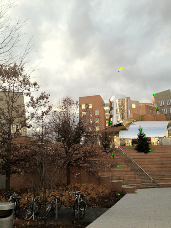
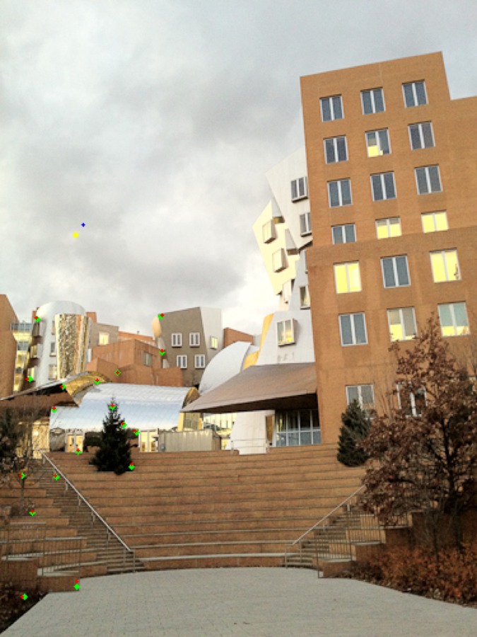
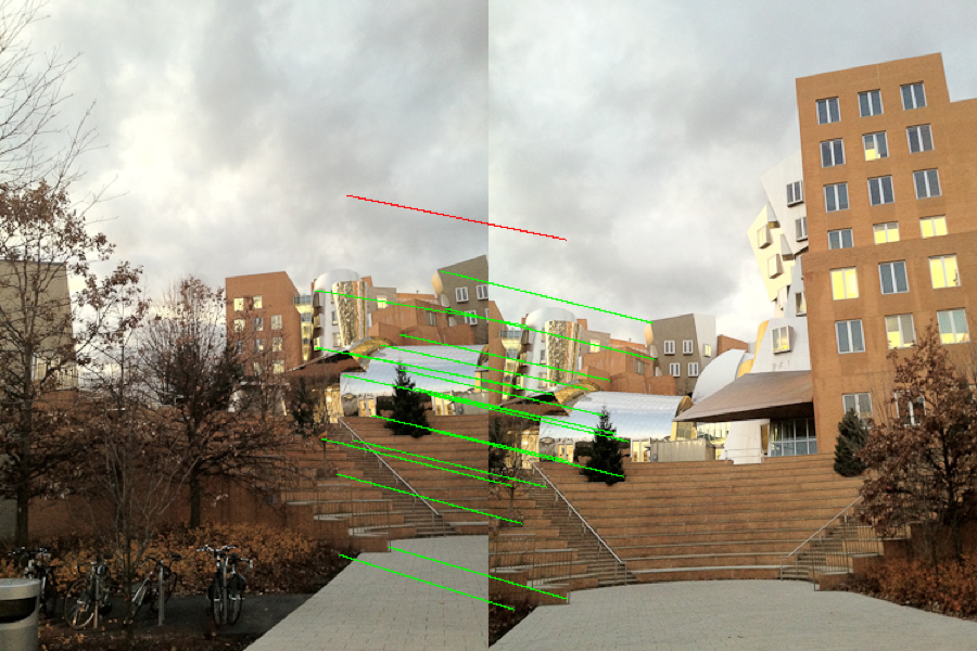
You can also use the provided visualizeReprojection, which shows where the homography reprojects features points. For inlier, detected corners are in green, while those re-projected from the other image are in red. For outliers, the local corners are yellow and the re-projected ones are blue. Our reproductions for Stata are below. The result below further emphasizes that RANSAC is probabilistic: the set of inliers is not exactly the same as above.

22.9.7 Automatic panorama stitching🔗⧉

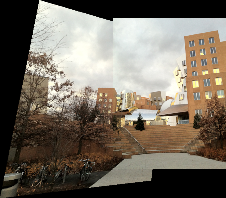
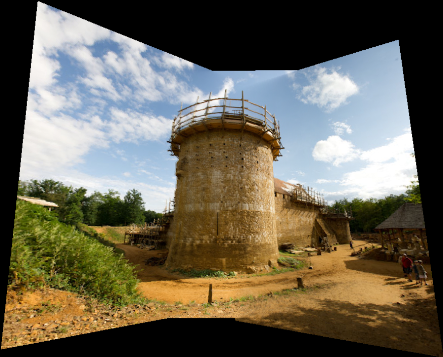
• Q. Write a function Image autostitch(const Image &im1, const Image &im2, float blurDescriptor, float radiusDescriptor) that takes two images as input and automatically outputs a panorama image where the first image is warped into the domain of the second one. You can and should call your problem set 6 functions in homography.cpp. You should get a similar-ish result to the last assignment (but automatically).

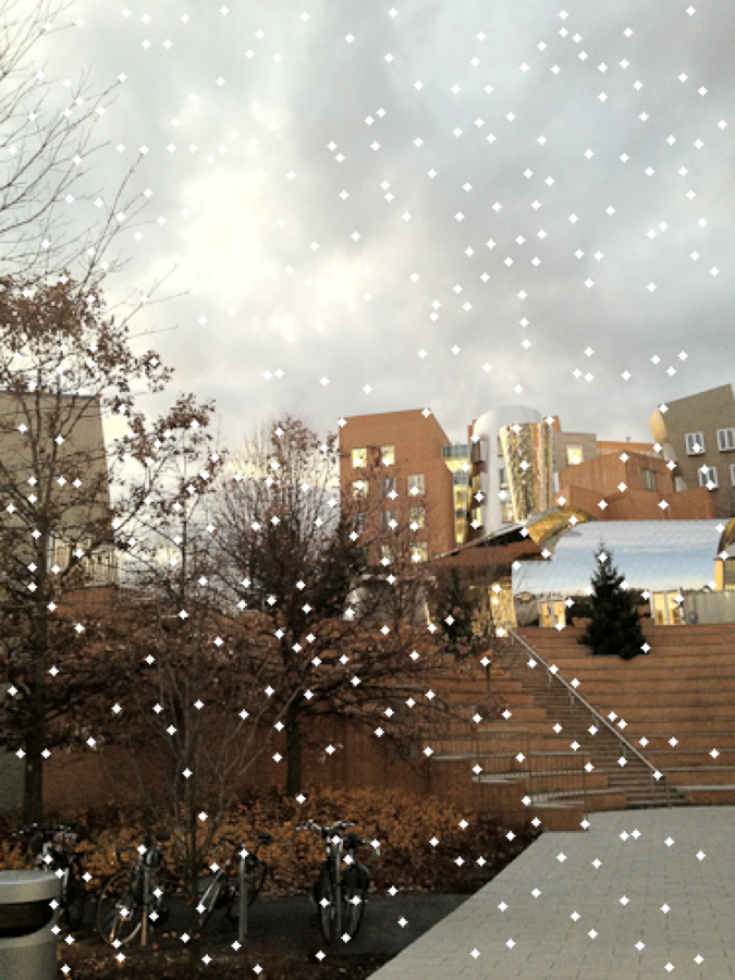
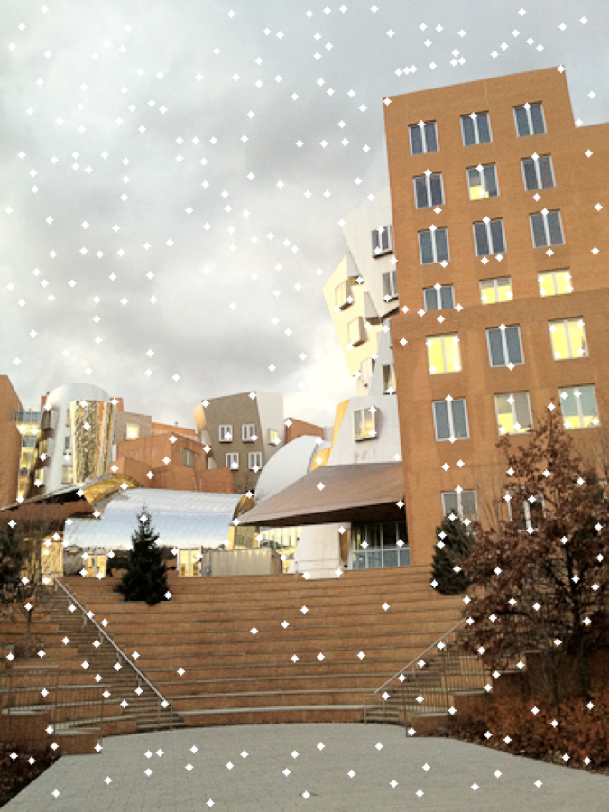
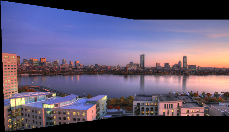
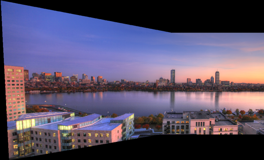
Try it on the Stata, Boston-skyline and at least another pair of images.

22.9.8 Blending🔗⧉

So far, we have re-projected input images into a common domain without paying much attention to problems at the boundaries. Our goal in this section is to mask the transition between images.

Linear blending🔗⧉

We will first implement a simple smooth transition between images. For this, the final output will be a weighted average of the reprojected inputs, where the weights decrease from 1 at the center of an image to 0 at the edges.

Weights are not easy to compute in the output domain because of the reprojection: it is harder to tell how far a pixel is from an image's boundary. Instead, we will compute the weights in the domain of the source image where it is trivial to tell how far a pixel is from the image boundary.

We will use piecewise linear weights in the source domain. The weights will be given by a separable function, which means that it is the product of a function only in $x$ and another function only in $y$. Each of these two functions will be piece-wise linear with a value of 1.0 in the center and 0.0 at the edges. For images with even width or height, the center doesn't have to be at a pixel (i.e. if the image has width 2, the center should be at 0.5).

• (a) Implement Image blendingweight(int imwidth, int imheight), which returns a single-channel Image of weights as described above.

We will now re-implement various functions from the last problem set with blending. Instead of directly copying the source values to the output we will add them weighted by the blend weight.

• (b) Implement void applyhomographyBlend(const Image &source, const Image &weight, Image &out, Matrix &H, bool bilinear), which is similar to applyHomography (or applyHomographyFast). But instead of directly writing the pixels of the input image to the output image, this function should add the pixels of the input image (source) times the weight to the output image.
• (c) Implement Image stitchLinearBlending(const Image &im1, const Image &im2, const Image &weight1, const Image &weight2, const Matrix &H), which stitches two images using the given weights. You can use applyhomographyBlend to help you with this. Note that stitch should not do any normalization -- if the two weights don't add up to 1 at some pixel, that's ok.

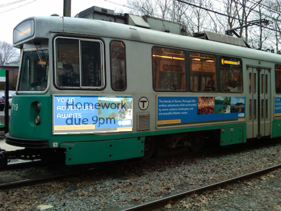
See the figure below for our weight map for the poster image, and our applyhomographyBlend applied to the green/poster combo with a constant weight of 0.5 for every pixel of the poster.

Better Blending🔗⧉

The problem with linear blending is that the resulting image can be blurry at the transition or exhibit ghosts when features are not exactly matched. To fix this, we will use a two-scale approach that uses smooth weights for the low frequencies and abrupt weights for the high frequencies.

We will achieve this by first decomposing the source image into low-frequency and high-frequency components. As we have done in the past, applying a Gaussian blur is sufficient to obtain the low-frequency, while the the high-frequency can be obtained by subtracting the low from the source.

Now that we have the individual components, we want to weight them accordingly. For the low frequencies use the same smooth weights we have used so far, e.g., blendingweight and combine them linearly. For the high-frequencies, use abrupt weights that only keep the high frequency of the image with the highest weight. That is, after warping the smooth weights of each image to the output domain, set the highest of the two weights to one and the lowest to zero. Linearly blend the images with these weights to obtain the blended high-frequency component. Finally compute the output image by adding the resulting low- and high-frequencies.

• (d) Implement stitchBlending(const Image &im1, const Image &im2, Matrix H, BlendType blend). Here BlendType is an enumerate taking the following values BLEND_NONE, BLEND_LINEAR, BLEND_2LAYER.
  • For BLEND_NONE the function should perform normal stitching (using im2 as reference, as was done in the previous problem set).
  • For BLEND_LINEAR stitch the two images using linear blending from above. Make sure you figure out some way of keeping track of the sum of the weights at each output pixel since (unlike above) we need the output of this function to be normalized.
  • For BLEND_2LAYER use 2-scale blending described above. For the Gaussian filter use a spatial sigma of 2 pixels (and default truncate/clamp parameters). You might find the function scaledecomp(const Image &im, float sigma = 2.0) useful. Hint: consider calling stitchBlending with various inputs to help with your implementation.

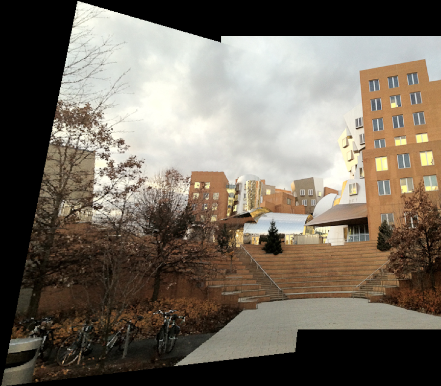
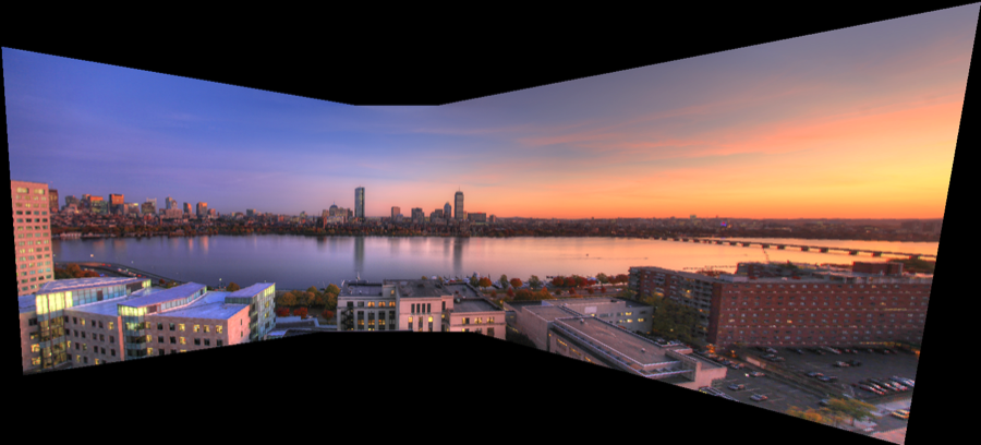
We now have all the pieces to obtain a fully automatic panorama stitching with blending! See it in action in the figure below for the Boston sequence (since we all know Boston skyline examples are cooler).

• (e) Implement Image autostitch(Image &im1, Image &im2, BlendType blend, float blurDescriptor=0.5, float radiusDescriptor=4), which is the same as the first part of the pset's autostitch, except it calls the stitch implementation above, with the fourth parameter blend. In other words, it computes features, finds correspondences, finds the homography (via RANSAC) before doing the stitch with the passed in blend type.

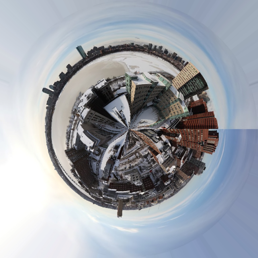
22.9.9 Mini planet🔗⧉

Assume you've been given a panorama image. Use the stereographic projection to yield the popular mini planet view. See e.g. <http://www.miniplanets.co.uk/> and <http://en.wikipedia.org/wiki/Stereographic_projection>.

• Q. Implement Image pano2planet(const Image &pano, int newImSize, bool clamp=true). Make a new image of square size (newImSize), and for each pixel (x, y) in the new image, compute the polar coordinates (angle, radius) assuming that the center is the floating point center as in blendingweights. Map the bottom of your input panorama to the center of the the new image and the top to a radius corresponding to the distance between the center and the right edge (in the square output). The left and right sides of the input panorama should be mapped to an angle of 0, along the right horizontal axis in the new image with increasing (counter-clockwise) angle in the output corresponding to sweeping from left to right of the input panorama. Assume standard polar coordinate conventions (angle is 0 along right horizontal axis and $\frac{\pi}{2}$ is along the top vertical axis). Use interpolateLin to copy pixels from panorama to planet image. Hint: see C++'s atan2.

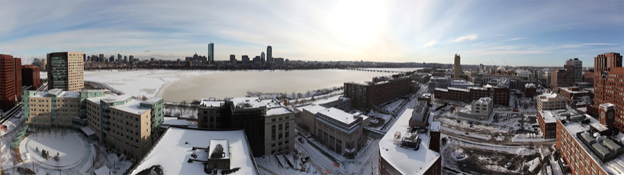
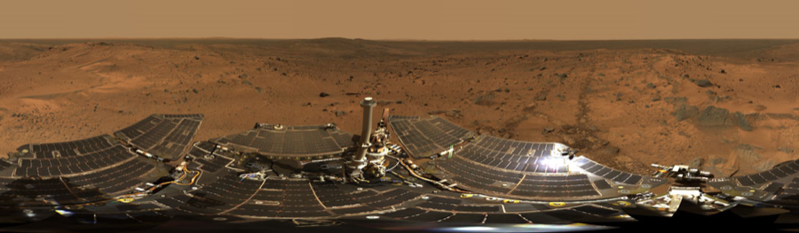
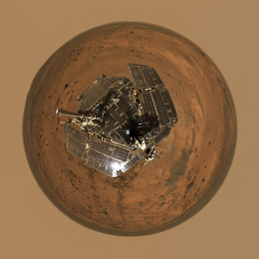
See the left side of the figure below for a winter panorama of Boston, and the resulting planet. Note that there is a rough line in the middle of the sky. This is because the panorama is not really 360 degrees. By contrast, the Mars panorama on the right side of the figure is 360, and we have a much smoother planet result.

22.9.10 6.8370: Stitch N Images (6.8371: Extra Credit 5%)🔗⧉

In this section you're going to compose a larger panorama using N images! Finally, some really fun stuff!

• (a) Implement vector<Matrix> sequenceHs(const vector<Image> &ims, float blurDescriptor=0.5, float radiusDescriptor=4); which computes a sequence of N-1 homographies for N images. H[i] should take ims[i] to ims[i+1]. Use the same pipeline we have used for individual homographies.
• (b) Implement vector<Matrix> stackHomographies(const vector<Matrix> &Hs, int refIndex);. This takes the N-1 homographies from the previous function, and translates them into N homographies for the N images. H[i] takes ims[i] to image ims[refIndex]. Therefore, H[refIndex] should be identity. Note that this requires some chaining of pairwise homographies to get the global homographies. Note that a different procedure is needed for images before and after the reference image.
• (c) Implement BoundingBox bboxN(const vector<Matrix> &Hs, const vector<Image> &ims);, which takes in N homographies and N images, and computes the overall bounding box.
• (d) Implement Image autostitchN(const vector<Image> &ims, int refIndex, float blurDescriptor=0.5, float radiusDescriptor=4);, which computes the sequence of homographies using sequenceHs then propagates them using stackHomographies function to the specified reference image refIndex. Then computes the overall bounding box using bboxN and the translation to make the box start at (0,0). Finally apply the homographies to all images to get the output panorama. Use linear blending. You can and should call your problem set 6 functions in homography.cpp.

22.9.11 Make your own panorama🔗⧉

Capture your own sequence of images and run it through your automatic algorithm. Two images for 6.8371, and at least three images (using N-stitching) for 6.8370.

Make sure you keep the camera horizontal enough because our naive descriptors are not invariant to rotation. Similarly, don't use a lens that is too wide angle (Don't push below a 35mm equivalent of 24mm). Your total panorama shouldn't be too wide angle (don't go too close to 180 degrees yet) because the distortions on the periphery would lead to a very distorted and ginormous output. Some of the provided sequences are already pushing it. Finally, recall that you should rotate around the center of projection as much as possible in order to avoid parallax errors. This is especially important when your scene has nearby objects.

If you need to convert images to .png, one online tool that appears to work is <http://www.coolutils.com/online/image-converter/>. Also, you might have to downsize your images since overly large images will take a long time to compute.

• (a) Turn in both your source images and your results in the folder my_pano of your submission zip file. Name your source images source_1.png, source_2.png... and name your final image mypano.png.

22.9.12 Extra credits (10% max)🔗⧉

For any extra credit you attempt (5% each), please write a new test function in your main file, and include the name of the test function in the submission questionnaire. This is a requirement for getting the extra credit.

Adaptive non-maximum suppression. See, for example, Section 3 in "Multi-Image Matching using Multi-Scale Oriented Patche", Brown et al 2005.

Wavelet or multi-scale descriptor.

Rotation or scale invariance for the descriptor.

Full SIFT. See "Object Recognition from Local Scale-Invariant Features", Lowe 1999.

Evaluation of repeatability of RANSAC.

Least square refinement of homography at the end of RANSAC.

Using iterative reweighted least square for handling outliers instead of RANSAC.

Bundle adjustment. See, for example, Section 4 in "Recognising Panoramas", Brown and Lowe 2003.

Automatically crop margins (5%). It's not trivial, but not too hard. Find a reasonable way to crop out the black margins automatically. Be careful not to crop too much from the Image.

Cylindrical reprojection (5%). We can reproject our panorama onto a virtual cylinder. This is particularly useful when the field of view becomes larger. This is not a difficult task per say, but it requires you to keep track of a number of coordinate systems and to perform the appropriate conversions. For this, it is best to think of the problem in terms of 3D projection onto planes vs. cylinders.

At the end of the day, we will start with cylindrical coordinates, turn them into 3D points/rays, and reproject them onto planar coordinate systems to lookup pixel values in the original images.

The projection matrix for a planar image when the optical axis is along the z coordinates is

where f is the normalized focal length, corresponding to a sensor of width 1.0.

This projects 3D points into 2D homogenous coordinates, which need to be divided by the 3rd component to yield Euclidean coordinates. The coordinates in the sensor plane are assumed to go from -0.5 to 0.5 for the longer dimension.

We then need to convert these normalized coordinates into [0..width, 0..height]. Define size=max(height, width), then the normalized coordinates

In the end, for the reference image, we have

We also know that for another image

Now that we have equations for planar projections, we compute the cylindrical projection of one image. We interpret the output pixel coordinates as cylindrical coordinates $y, \theta$ (after potential scaling and translation). $y$ is the vertical dimension of the cylinder and $\theta$ the angle in radian. We convert these into a 3D point $P_{3D}$, which we reproject into the source image where we perform a bilinear reconstruction.

We encourage to debug this using manually-set bounding boxes (e.g. $-\pi/2..\pi/2$ in $\theta$, and a scaling factor that maps preserves the height of the reference image).

You can then, if you want adapt your bounding box computation. Note that cylindrical projections are not convex, and taking the projection of the 4 corners does not bound the projection. You can ignore this and accept some cropping or sample the image boundary more finely.

Horizon correction for cylindrical reprojection (5%). The $y$ axis of the reference image is not necessarily the vertical axis of the world. This might result in some distorted reproduction where the horizon is not horizontal.

You can address this by fitting a plane onto the centers of the panorama source images in the 3D coordinate system of the reference image.