3.8 Resampling⧉
Resizing an image is the most ordinary thing you ever ask of an editor — shrink a photo for the web, zoom into a crop, straighten a tilted horizon, undo lens distortion. It feels like it should be a one-liner. To make a picture twice as big you spread the pixels out; to make it smaller you throw some away. The whole point of this chapter is that both of those instincts are wrong, and that doing the job well — well enough that you could rotate an image three hundred times without it dissolving — quietly leans on everything we built in the convolution and Fourier chapters.
The reason is that an image is not a picture, it is a grid of samples: point measurements of an underlying continuous scene. When you resize, you ask for the scene's value at new positions that fall between the samples you actually recorded. No pixel lives there to copy. So the honest statement of the problem has two steps — reconstruct a continuous signal from the samples you have, then re-sample it wherever the new grid asks for a value. Hold onto that sentence. It is the spine of the chapter, and every method below is just a different answer to "how should I reconstruct?"
3.8.1 Domain operations: moving pixels around⧉
Recall the three families of image operation from the point-operations chapter, sorted by what each output pixel is allowed to read. Resampling is the domain family: the colors are left alone, only the positions move. Formally a domain transform applies a function $f$ from the plane to itself — from $\mathbb{R}^2$ to $\mathbb{R}^2$ — to the image's coordinates, with the rule that if the point $(x,y)$ carried color $c$ in the input, then $f(x,y)$ carries that same color $c$ in the output. The range (the colors) is untouched; only the domain (the coordinates) is remapped.
That one definition spans a huge amount of ground. When $f$ is a uniform scale it is resizing; a rotation straightens a horizon; an affine or perspective $f$ fixes keystoning or stitches a panorama; and a freely chosen $f$ is a warp — picture the image printed on rubber and stretched. The genuinely free-form case, including how a user even specifies such an $f$ (and the morphing it unlocks), gets its own warping chapter. Here we take $f$ as given and concentrate on the hard part shared by every domain transform: the new positions almost never land on the input grid, so we must invent values between the samples.
3.8.2 Start with scaling up⧉
Start with the friendliest case, scaling an image up — say by an integer factor $k$. The output has $k$ times as many pixels along each axis, so most output pixels sit between input pixels and have no value of their own: we have too few samples and must fill in the gaps. (Downsampling is the opposite complaint — too many input samples crowding into each output pixel — and, surprisingly, it needs a slightly different fix. Hold that thought; the pleasant punchline is that the machinery turns out to be almost identical.) Upsampling is the cleaner place to build intuition, so we begin there.
3.8.3 The naive idea, and why it leaves gaps⧉
Here is the instinct nearly everyone has first: loop over the input pixels, and for each one compute where it lands in the output and write its color there. To scale up by $k$, the input pixel at $(x,y)$ goes to output location $(k\,x,\ k\,y)$:
This is forward mapping — push each input pixel forward to its destination. It is intuitive, and it is broken. Scale up by $k=2$ and you write output pixels $(0,0),(2,0),(4,0),\dots$ while every odd-coordinate pixel is never touched: a regular lattice of black holes (Figure 3.8.1, left). The output is mostly gaps, because spreading $N$ input pixels over $k^2 N$ output positions can fill at most $N$ of them — one cell of every $2\times2$ block, three left empty.
You might try to patch it with an inner loop that paints the little square between four placed pixels. That limps along for an axis-aligned enlargement, but the instant $f$ is a rotation the gaps stop being neat squares — they become slivers at odd angles, and "fill the gap" no longer has an easy shape. Forward mapping fights you. We need a different loop.

3.8.4 Loop over the output, use the inverse transform⧉
The fix is to turn the loop inside out. Instead of pushing inputs forward, iterate over the output pixels — all of them, so none can be skipped — and for each one ask where did this come from in the input? That means applying the inverse transform $f^{-1}$ to the output coordinate and reading the input there:
For a scale-up by $k$ the inverse divides by $k$, so output pixel $(x,y)$ reads the input at $(x/k,\ y/k)$. Now every output pixel receives exactly one value and there are no gaps by construction. This is inverse mapping, and the lesson deserves to be stated flatly: loop over output pixels, and always use the inverse transform. It is the same "where-from, not where-to" reflex as the flip in convolution — to fill a destination, reach back into the source — and it is the single most important habit in this chapter. (Figure 3.8.1 sets the two loops side by side.)
There is one immediate wrinkle, and it is the real subject of everything that follows. Inverse mapping is clean, but $f^{-1}(x,y)$ lands at a fractional coordinate — $(x/k,y/k)$ is rarely an integer, and under a rotation it essentially never is. There is no pixel sitting at $(1.3, 4.7)$. So the genuine content of resampling is the question we have been circling: given the input samples, what value should we report at a position between them? Every method below is one answer.
3.8.5 Nearest neighbour⧉
The crudest answer: round the fractional coordinate to the closest integer and copy that pixel. Want the value at $1.3$? Round to $1$, return $I[1]$. This is nearest-neighbour reconstruction, and it is exactly what we were silently doing when we wrote $I[x/k,\,y/k]$ and let integer indexing truncate the coordinate.
It works and it is fast, but the result is conspicuously blocky: a whole range of fractional positions all snap to the same input pixel, so an upscaled image looks like fat rectangular tiles (Figure 3.8.12, nearest panel), each input pixel becoming a hard $k\times k$ block. Occasionally that is precisely what you want — pixel art, or a debug view where you want to see the literal samples — but as a general-purpose resize it is the floor, not the goal. As the challenge for nearest neighbour: try upscaling a face by $8\times$ this way and watch it turn to mosaic. We do much better by interpolating between samples instead of snapping to one.
3.8.6 Linear interpolation, in 1-D first⧉
Drop to one dimension, where the idea is cleanest. An image row is a 1-D array of values, and we want the value at $1.3$, between the samples at $1$ and $2$. The natural move is to blend the two neighbours in proportion to how close the query sits to each. At $1.3$ we are $0.3$ of the way from $1$ toward $2$, so
This is linear interpolation, and there is one detail that trips up everyone at first: the weights run opposite to the distances. The neighbour you are $0.3$ away from gets weight $0.7$, not $0.3$ — because you want weight $1$ when you sit exactly on a sample and $0$ when you are a full step away. Say it back in words: take a weighted average of the two bracketing samples, weighting each by one minus the distance to it. Geometrically, the reconstructed signal is just the straight line connecting consecutive samples (Figure 3.8.2).

3.8.7 Bilinear, in 2-D⧉
In two dimensions we now have four surrounding samples — the corners of the unit square the query falls inside — and two fractional coordinates to interpolate against. The clean construction is to do 1-D linear interpolation twice: first along $x$, then along $y$ (Figure 3.8.4). Blend the top pair of pixels horizontally to get one value, blend the bottom pair horizontally to get another, then blend those two results vertically with the $y$ fraction. The four corner weights come out as products of the $x$- and $y$-blend factors — which is exactly why this is bilinear: linear in each axis, but their product, not a single plane through all four points.
That last point is a real subtlety worth a pause. Four arbitrary corner values do not in general lie on a flat plane, so a "purely linear" 2-D surface through all four simply does not exist. Bilinear sidesteps this by being linear separately in each direction (the product of two tents), which is well-defined and cheap. The resulting surface is doubly ruled — dead straight along every horizontal and every vertical line, yet curved overall, twisting into a saddle when the four corners disagree (Figure 3.8.4b). The only way to get a truly planar piecewise-linear reconstruction is to triangulate — cut each square into two triangles and interpolate within each, since three corners do fix a plane.


If you do triangulate, you must choose which diagonal to cut each square along, and the two choices differ near edges. A naive splitter always cuts the same way, secretly preferring one diagonal and producing a faint directional bias. The smarter trick picks, per square, the diagonal joining the two most similar corner values — cutting along an edge rather than across it, so a sharp boundary isn't smeared. Bilinear's quiet advantage is that it has no diagonal to choose: it needs no branch and favours no direction.
Show that interpolating $y$ first, then $x$ gives exactly the same result as $x$ first, then $y$. (Write both as weighted sums of the four corners and compare the coefficients — the order of the two separable passes does not matter.)
Putting the two halves together — the inverse-mapping loop and the bilinear sample — gives the whole upsampler. Loop over output pixels, send each back through $f^{-1}$ to a fractional input location, split that into its integer cell and fractional offsets, and blend the four corners:
for each output pixel (x, y):
    (u, v) = f⁻¹(x, y)                  # fractional input location
    x0, y0 = floor(u), floor(v)
    s, t = u - x0, v - y0               # fractional offsets in [0, 1)
    top = (1 - s)·I[x0, y0]   + s·I[x0+1, y0]
    bot = (1 - s)·I[x0, y0+1] + s·I[x0+1, y0+1]
    out[x, y] = (1 - t)·top + t·bot     # blend the two rows vertically
Read it back: the two horizontal blends collapse the top and bottom edges of the cell, and the final vertical blend combines them — 1-D linear interpolation done twice. Bilinear is the workhorse default: cheap, no blocky tiles, smooth enough for most resizing, and the reconstruction you get for free from a graphics-hardware texture lookup (Figure 3.8.12, bilinear panel). But it has a ceiling. The reconstructed surface has creases — it is only continuous, not smooth, kinking at every sample — and on a strong upscale it reads a touch soft. To push past it we need to look at more than four neighbours, and the "interpolate between neighbours" story does not generalize gracefully. We need a better lens — but first a word on what any of this costs.
In general you cannot precompute the kernel weights: because $f^{-1}$ lands at arbitrary fractional offsets, every output pixel may need the kernel evaluated at different points (expect to re-evaluate it per output pixel, per neighbour). Two things rescue performance. First, the kernels are separable — a 2-D resample is a horizontal pass then a vertical pass, turning an $r\times r$ cost into $2r$ — so the standard implementation scales in $x$, producing an anisotropically-stretched intermediate, then scales in $y$. Second, for an integer scale factor the fractional offsets repeat, so the weights can be precomputed and the whole thing collapses to an ordinary discrete convolution. Andrew Adams' advice for downsampling is exactly this: build the tiny sparse weight matrix that downsamples a single row (the weights repeat for every row), normalize each row to sum to $1$ — which conveniently also fixes the borders — and apply it everywhere; and because the reduction is separable, do the shrinking pass first so the second pass works on less data.
3.8.8 The convolution perspective⧉
Here is the reframing that unlocks everything. So far we have described reconstruction as interpolating between neighbours. That picture is fine for linear interpolation and for upsampling, but it has two failings: it does not extend cleanly to fancier reconstructions, and — crucially — it does not extend to downsampling at all. Since this whole chapter is fundamentally about (re)sampling, the Fourier-flavoured view from the aliasing chapter has much better insight to offer. In practice that view means one thing: reconstruction is convolution.
Concretely, the output value at a fractional location is a weighted average of nearby input pixels, with the weights read off a smooth analytical kernel $k$ centred at the desired (non-integer) location. Slide a continuous kernel so its centre sits exactly on the query point $f^{-1}(x,y)$, evaluate the kernel at each surrounding integer input pixel to get that pixel's weight, and sum. The general resampling formula is
summing over input pixels $x'$ in the neighbourhood, the kernel evaluated at the offset between the query and each pixel. In words: to find an output pixel, inverse-transform it to a fractional input location, drop a smooth kernel centred there, and accumulate kernel-weight times pixel-value over the nearby samples. It is convolution — but where convolution in the earlier chapter lived purely on the integer grid, here the kernel is a continuous function we can evaluate at any fractional offset (ask for $k(-0.7)$ and it answers), because the centre is non-integer.
This is the place to be emphatic about a requirement easy to skate past: because resampling evaluates the kernel at non-integer positions — the output sample falls between the input samples, so the offset $f^{-1}(x,y)-x'$ is essentially never an integer — the kernel must be a continuous, analytic function of a real argument, $k(x)$, that you can evaluate anywhere, not a discrete list of taps. A fixed convolution stencil (a $[1,4,6,4,1]/16$ blur, say) only has values at integer offsets; ask it for $k(-0.7)$ and it has nothing to say. This is the whole reason resampling kernels are written as closed-form functions — cubic polynomials, windowed sincs — rather than tap lists: you need a formula you can sample at the exact fractional offset every output pixel demands (Figure A).

The beauty is that bilinear is already a special case. The linear-interpolation weights $0.7$ and $0.3$ are exactly the values of a triangular (tent) kernel — one that is $1$ at its centre and falls linearly to $0$ one sample away on each side — evaluated at the offsets to the two neighbours. So "interpolate linearly" and "convolve with a tent" are the same operation, seen two ways. Nearest neighbour is the same story with a box kernel (a flat $1$ over a one-pixel window). Once reconstruction is "convolve with a kernel," choosing a better reconstruction is just choosing a better kernel.
The fully honest pipeline has three stages, not one (Figure B). Start from the sampled input. 1/ Reconstruct a continuous signal with a reconstruction filter. 2/ Prefilter (low-pass / blur) it so it carries no detail too fine for the output grid to represent — the anti-aliasing step from the aliasing chapter. 3/ Resample on the output grid. Because both the reconstruction and the prefilter are convolutions, they combine into a single kernel — the final filter is the prefilter composed with the reconstruction filter — which is why one piece of code does the whole job. Which factor dominates that combined kernel depends on direction: upsampling is dominated by the reconstruction filter (the output grid is fine, so little prefiltering is needed); downsampling is dominated by the prefilter (we must aggressively strip detail the coarse grid cannot hold). Same machinery, opposite emphasis.

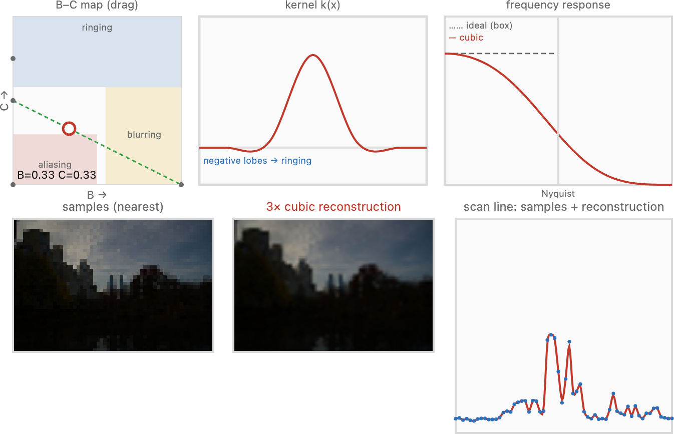
3.8.9 Better kernels: bicubic and Lanczos⧉
If the kernel is what matters, what makes a good one? The theoretical answer, straight from the sampling chapter, is the sinc function, $\operatorname{sinc}(x)=\sin(\pi x)/(\pi x)$: it is the kernel whose Fourier transform is a perfect box, passing every frequency the grid can represent and rejecting every one it cannot, exactly. Sinc is the single mathematically optimal reconstruction filter. The catch — fatal in practice — is that sinc is infinitely wide, assuming an infinite image and an infinite compute budget. You cannot afford a kernel that reaches across the whole image for every output pixel, and it rings badly when truncated.
So every practical reconstruction kernel is an approximation of sinc with finite support, balancing two competing evils that are clearest in the frequency domain (the perfect-box-versus-smooth-approximation picture from the aliasing chapter). A kernel that is too gentle loses medium frequencies — its response rolls off early and the image goes soft — while one too aggressive lets high frequencies alias — it leaks past the grid's limit and admits jaggies and moiré. Every kernel is a point on this blur-versus-alias tradeoff. The two famous families both live on it.
Lanczos is sinc literally windowed by a wider sinc:
over a support of $a$ samples on each side (and zero beyond). It hugs the ideal closely and looks crisp, at the cost of some ringing near strong edges — the surviving side-lobes of the truncated sinc (Figure C).

Bicubic uses a piecewise cubic polynomial — smooth, compact (four samples wide in 1-D), the standard default in image editors. It typically carries small negative lobes to the sides, and those are not a bug: they give the reconstruction a built-in mild sharpening (much like the unsharp mask) that makes upscaled images crisper. The cubic kernel is not unique — there is a family. Once you impose the natural requirements — the kernel should be symmetric, should be smooth where the cubic pieces meet, and should sum to one so it preserves brightness — a cubic still has two free parameters left. Mitchell and Netravali (1988) named them $B$ and $C$; the result is a single piecewise cubic, supported over four samples (two on each side):
one cubic whose two knobs slide it between sharper and smoother. Three points of the $(B,C)$ plane are the canonical members worth knowing by name:
- $(B,C)=(1,0)$ — the cubic B-spline: the smoothest member, all-positive (no negative lobes), and approximating rather than interpolating, so it visibly blurs;
- $(B,C)=(0,\tfrac12)$ — Catmull–Rom: interpolating (it passes exactly through the samples) with pronounced negative lobes, so it looks sharp;
- $(B,C)=(\tfrac13,\tfrac13)$ — Mitchell–Netravali: the balanced default, sitting between the two and minimizing the combined visible artefacts.


Mitchell and Netravali (1988) found their balance by running a perceptual study mapping which $(B,C)$ choices look best, charting where each lands among three failure modes: residual blur (too little negative lobe), ringing (ghost edges from too-strong negative lobes), and anisotropy (a visible preference for the horizontal / vertical / diagonal directions). A broad region of the $(B,C)$ map looks satisfactory, but different points suit different images — which is exactly why Photoshop and friends offer you a choice of bicubic ("bicubic smoother" for enlargements, "bicubic sharper" for reductions) rather than one fixed filter. There is no universally best answer, only a tradeoff you tune to the image: a slightly blurry original can afford a sharper kernel, a crisp one cannot.
Real software exposes exactly these kernel choices. Photoshop's Image Size resample menu lets you pick Nearest Neighbor, Bilinear, Bicubic, Bicubic Smoother (for enlargements), Bicubic Sharper (for reductions), and Preserve Details — the very box / tent / cubic family, and the smooth-versus-sharp bicubic tradeoff, turned into a dropdown (Figure F).

Bicubic is not "fit a cubic polynomial through the data points." It is convolution with a fixed cubic kernel — a reconstruction filter, not a curve fit. The confusion is widespread: blog posts, textbooks, and historically shipping software (old Python imaging libraries among them). If a description says it interpolates by fitting a cubic through the pixels, distrust it. Resampling — and downsampling especially — is notoriously easy to get subtly wrong and hard to debug, because the output still looks like an image, just a slightly bad one. The stakes are not merely cosmetic. Broken, aliased resizing in standard image libraries silently corrupts the metrics used to evaluate generative models (arXiv:2104.11222) and is an outright security hole (arXiv:2104.08690). The worst offender is nearest-neighbour downsampling with no prefilter: because it keeps one input pixel per output pixel and discards the rest, an attacker who knows the target size can plant a sparse lattice of tiny, near-invisible dots positioned to land exactly on the kept sample grid — so the decimated result is a different picture entirely (Figure G). Prefilter-free decimation is not just blurry-in-a-bad-way; it is broken enough to hijack.


3.8.10 Upsampling vs. downsampling: scale the kernel⧉
We have promised twice that downsampling reuses the same machinery; now we cash it in. Whether you scale up or down, you run the same convolution with the same family of kernels. The only thing that changes is how you scale the kernel.
When upsampling, the kernel keeps a fixed footprint in the input image — about four pixels wide for bicubic, however much you enlarge — because the input samples are already dense enough; you are just reading between them. So for upsampling the kernel width in input space is constant (a useful corollary: clamp the kernel's scale factor at $1$, never narrower).
Downsampling is the genuinely harder case, and not by a little. Pick one input pixel per output pixel — nearest neighbour, no blur — and you get aliasing: a fine texture turns into bold, wrong, low-frequency moiré (a brick wall or a striped shirt shot from far away dissolving into wide phantom bands; Figure 3.8.16). This is not a cosmetic glitch but the wagon-wheel / Prudential-tower effect from the aliasing chapter: detail finer than the output grid can represent does not vanish, it folds down and masquerades as coarse structure.
The cure is exactly the anti-aliasing rule from that chapter: blur before you downsample. Average the input over the footprint of each new, larger output pixel, so the only patterns surviving into the small image are ones it can actually represent; then sample. Mechanically this is the same kernel as upsampling, scaled up in input space: the more aggressively you shrink, the wider the kernel must reach, because we want it to stay a roughly fixed size in output space — so it has to span more and more input pixels and average over all of them. Downsample by $5\times$ and each output pixel should gather roughly a $5$-pixel-wide neighbourhood. So the whole up / down distinction collapses to one knob: keep the kernel fixed in input space to upsample, grow it in proportion to the scale factor to downsample. One code path, one kernel-scale parameter (Figure 3.8.15).


The effect is ugliest on real, regular structure — the rows of windows on a glass facade, shrunk for a thumbnail, break into sweeping moiré if you decimate without prefiltering (Figure 3.8.17).

3.8.11 Prefiltering when the transform isn't a clean scale⧉
Everything above quietly assumed a uniform scale, where the right prefilter is the same everywhere and radially symmetric — the same in every direction, a round footprint. For a shear, rotation, or perspective (homography) that assumption breaks. Back-project a single square output pixel through $f^{-1}$ and its footprint in the input is no longer round: under an affine map it becomes a stretched, tilted ellipse, elongated in whatever direction the transform compresses most. So the ideal prefilter is not a circle but that ellipse — anisotropic and position-dependent, a different shape at every pixel. Doing it exactly is therefore spatially varying and anisotropic, which is genuinely expensive. In practice we approximate it: mip-maps (a precomputed pyramid of progressively blurred, downsampled copies — see pyramids) let hardware pick a roughly-right isotropic blur level cheaply, and elliptical weighted average (EWA) filtering approximates the true back-projected ellipse more faithfully when quality matters. The takeaway for now: the clean "scale the kernel" story is the easy case, and non-uniform transforms need an anisotropic, position-dependent prefilter we can only approximate.
Here is a stress test that exposes a resampler instantly: rotate an image all the way around in $N$ equal steps — rotate $N$ times by $360/N$ degrees — so the geometry returns the image to its original orientation and a perfect resampler would hand back (nearly) the original picture. The point is to try several $N$ (the figure shows $N=10$, $60$, and $360$): the more steps you take, the more times the image is resampled, and the more — smaller — rotations compound more damage, not less. Crucially you rotate $k$ times by $360/N$ each; you never do a single rotation by $k\cdot 360/N$, which would resample only once. A naive resampler — repeated bilinear with no proper prefilter — blurs a little on every step, and those tiny blurs compound into mush; the image dissolves, worse at larger $N$. A good resampler (a proper prefilter plus a sharp-but-stable reconstruction kernel) keeps the errors from accumulating and returns something very close to the start even after $360$ rounds. It is a brutal, honest way to compare resampling quality: errors invisible once become glaring after a few hundred rounds.

3.8.12 Where this goes next⧉
We end where the chapter began: resampling is reconstruct-then-resample, and reconstruction is convolution with a kernel that approximates sinc on a finite budget. That one idea recurs immediately. The blur-then-downsample reduce step is the engine of the Gaussian and Laplacian pyramids, the next chapter. The inverse-mapping discipline — loop over output, apply $f^{-1}$, reconstruct — is exactly what general warping and morphing will need once we let the user specify an arbitrary $f$. And a resampler's quality is one of the things we will quantify when we reach image metrics. The mechanics are humble — a weighted average of a handful of neighbours — but, as the rotation challenge shows, getting that weighted average right is what separates a tool you can trust from one that quietly destroys your image.