4.5 Generative AI and diffusion🔗⧉

This chapter is the generative limit of the two before it. Linear inverse problems laid down the template every recovery task in the book reuses: fit the data, lean on a prior, solve. Machine learning swapped the hand-designed prior for one learned from data (L8). Super-resolution — over in the single-image part — pushed further: it showed that the prior is not optional once the measurement has destroyed information (L10), and that a humble denoiser is a universal prior you can plug into any solver — the plug-and-play (PnP) and regularization by denoising (RED) idea. Here the prior takes one final step. It becomes something you can sample from — a generative model — and the canonical generative model, diffusion, turns out to be precisely that denoiser run in a loop. We point to the machine-learning refresher (Refreshers#Machine learning and deep learning) for the network machinery; this chapter surveys the generative idea and, above all, where it plugs back into the book's inverse-problem spine.

4.5.1 The framing: generation is learning and sampling a prior $p(x)$🔗⧉

Every prior we have used so far is something you evaluate. It is a penalty $\Phi(x)$ you add to a data term, as in $\min_x \tfrac12\|Ax-y\|^2 + \lambda\,\Phi(x)$, scoring a candidate image as "smooth enough" or "natural enough." Or it is a denoiser you plug into a solver — the PnP/RED move from Super-resolution, where each iteration cleans the running guess a little. Either way, you may ask the prior "how good is this image?", but never "give me an image." A generative model can answer the second question. It learns the distribution of natural images $p(x)$ well enough that you can draw a fresh sample from it, written $x \sim p(x)$ — not score an image someone hands you, but produce one out of nothing (Figure 4.5.1).

That single shift — from scoring an image to drawing one — unlocks three capabilities at once, and they organize everything below. First, unconditional generation: invent a plausible photograph from nothing. Second, conditioning: sample not from $p(x)$ but from $p(x \mid c)$, the distribution of images consistent with a condition $c$ of your choosing — a text prompt, a sketch, a class label, another image. This is text→image and image→image. Third, and most consequential for the rest of this book, posterior sampling: condition the prior on an actual measurement $y$ and draw from $p(x \mid y) \propto p(y \mid x)\,p(x)$ — which is exactly super-resolution, deblurring, and inpainting carried out with the strongest prior we have. The inverse-problem template never changes; the prior simply learned to generate.

Why does sampling matter so much for restoration? Because so many of these tasks are one-to-many. Colorize a grayscale photo, super-resolve a thumbnail, fill a hole left by a removed object — in each case many sharp images explain the one degraded input equally well. A regression network trained with a squared-error loss, asked for the single "best" answer, hedges: it returns the average of all those plausible images, and the average of many sharp images is a blurry one. That is the mushy-mean failure flagged back in Deep learning. A generative prior does not average. It samples one sharp, plausible answer — and, run again, a different one (Figure 4.5.6, later).

A closing note before the math: the instinct to "sample plausible pixels" predates deep learning by two decades. Efros–Leung texture synthesis (Efros & Leung 1999) grew a new image one pixel at a time, each pixel copied from a real patch whose neighborhood best matched the already-synthesized surroundings — a non-parametric draw from the patch distribution, with no learned model at all. Same instinct (sample from $p(x)$), done by lookup. The lineage that runs through GANs and VAEs (placed at the chapter's end) and lands on diffusion is the story of learning that distribution rather than copying from a single image.

4.5.2 Diffusion: generation as iterated denoising🔗⧉

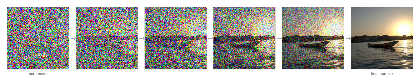
Diffusion is the generative model that now dominates image synthesis, and its mechanism is the one this entire part has been circling. The intuition is a single sentence: to generate an image, start from pure noise and denoise it, a little at a time, until a picture appears. Everything else is making that precise. It is built from two chains running in opposite directions (Figure 4.5.2).

The forward chain is fixed and requires no learning: it slowly destroys an image by adding Gaussian noise. Start from a clean photo $x_0$ and, step by step, blend in more noise until — after $T$ steps — nothing remains but static, $x_T \sim \mathcal{N}(0, I)$. This variance-preserving forward process has a tidy closed form that jumps straight to any noise level $t$:

In words: at level $t$, the corrupted image $x_t$ is the clean image scaled down by $\sqrt{\bar\alpha_t}$, plus a dose of fresh Gaussian noise $\epsilon$ scaled by $\sqrt{1-\bar\alpha_t}$. The schedule $\bar\alpha_t$ slides from nearly $1$ at $t=0$ (essentially the clean image) to nearly $0$ at $t=T$ (essentially pure noise). Note the bookkeeping that "variance-preserving" buys us: the clean image is shrunk by $\sqrt{\bar\alpha_t}$ as the noise grows, so the total scale stays bounded. The reverse chain is where the learning lives: a network that, given a noisy $x_t$ and its level $t$, removes a little of the noise to step back toward $x_{t-1}$. Sampling then means starting from pure static $x_T \sim \mathcal{N}(0,I)$ and running the reverse chain all the way down to a clean $x_0$ — an image emerging from noise.

What does the network actually learn? Surprisingly little, and it is the same thing at every level: predict the noise. Write the network $\epsilon_\theta(x_t, t)$ and train it — over clean images, random noise samples, and random levels — to recover the noise that was added. This is the denoising diffusion probabilistic model (DDPM) training objective (Ho, Jain & Abbeel 2020):

This is ordinary squared-error regression with the noise $\epsilon$ as the target. But predicting the noise is denoising: subtract the predicted noise from $x_t$ and you have an estimate of the clean image. So the trained network is nothing more exotic than a denoiser that works at every noise level — one model, one level input, trained to clean images however badly they are corrupted. (The network itself is a U-Net or transformer; the Refreshers cover both.)

Now the hinge of the whole chapter — the identity that ties diffusion back to everything else in the book. For a Gaussian-noised image under the variance-preserving forward process, the best possible denoiser — the one returning the posterior-mean estimate of the clean image — is given by Tweedie's formula:

The quantity $\nabla_{x_t}\log p(x_t)$ is the score: the gradient of the log-density, the direction in image space that points "uphill" toward more probable images. Tweedie says this score and a Gaussian denoiser are the same object, one rearranged into the other. The denoiser's correction — the vector from the noisy image toward the clean estimate — is the score, weighted by the noise variance $1-\bar\alpha_t$ and then rescaled by $1/\sqrt{\bar\alpha_t}$ to undo the variance-preserving shrinkage of $x_0$ (Figure 4.5.3). A trained diffusion model is therefore, equivalently, a learned score field (Song et al. 2021): at every noise level it tells you which way points toward the manifold of natural images. (This identity first appears in Denoising as a universal prior, Super-resolution and image priors; here it is the spine.)

Spelled out as a loop, sampling starts from pure static and walks the schedule down to a clean image:

x ← sample from 𝒩(0, I)              # pure noise, the endpoint x_T
for t from T down to 1:
    ε̂ ← ε_θ(x, t)                    # predict the noise at this level
    x ← denoise_step(x, ε̂, t)        # subtract a little, rescale by the schedule
    if t > 1:
        x ← x + σ_t · 𝒩(0, I)        # reinject a little fresh noise — sample, don't average
return x                              # the clean image x_0

Read it back: at each level the network predicts the noise, the step removes a little of it, and a dab of fresh noise is added back so the walk samples one sharp image rather than collapsing to the blurry mean.

This is why diffusion is PnP/RED taken to its continuous limit. The reverse sampling loop — denoise a little, add a little fresh noise, step down the noise schedule, repeat — is structurally the Plug-and-Play / RED outer loop from Super-resolution (Venkatakrishnan et al. 2013; Romano et al. 2017), with the plug-in denoiser being the learned score evaluated over a whole schedule of noise levels instead of at one fixed level. Generation is iterated denoising. The book's universal-denoiser-as-prior abstraction and its most powerful generative model are, mechanically, the same thing. Seen this way, every solver in the book fills one prior slot with a denoiser, and the available choices form a spectrum of increasing strength — a hand-built smoother, a classical denoiser, a learned convolutional neural network (CNN), and finally the diffusion score at the far end (Figure 4.5.7, anchored in the next section).

The naïve version runs all of this in pixel space, which is expensive at high resolution. Latent diffusion (Rombach et al. 2022, the basis of Stable Diffusion) makes it cheap (Figure 4.5.4). First an autoencoder encodes the image into a compact latent $z = \mathcal{E}(x)$ — a far smaller tensor that discards imperceptible detail. The entire diffusion process, forward and reverse, then runs in that latent space. A final decode $x = \mathcal{D}(z)$ turns the generated latent back into a full-resolution image. Diffusing a small latent rather than millions of pixels is what made open, high-resolution text→image generation practical on ordinary hardware.

4.5.3 Conditioning: text, images, and control🔗⧉

So far the model samples from $p(x)$ — any plausible image. The capability everyone actually wants is to steer it: sample from $p(x \mid c)$ for a condition $c$ of your choosing.

Text→image is the headline. A frozen text encoder — CLIP (Contrastive Language–Image Pre-training) or a large language model — turns the prompt into a sequence of embeddings, and those embeddings condition the denoiser at every reverse step through cross-attention (the attention machinery is the Refreshers' job). The model now samples from $p(x \mid \text{text})$ rather than $p(x)$. This is the engine of Stable Diffusion, DALL-E, and Imagen-style systems.

It is worth pausing on why text and images call for different generative models — the answer is structural, not fashion. Text is a sequence of discrete tokens from a finite vocabulary, with a natural left-to-right order, which is a perfect fit for autoregressive language models that factor the distribution as $p(x) = \prod_i p(x_i \mid x_{<i})$ and predict one token at a time with an exact next-token likelihood. Images are continuous, million-dimensional, and have no canonical ordering — there is no natural "first pixel" — which is a perfect fit for diffusion, which adds and removes continuous Gaussian noise across all pixels in parallel and needs no ordering at all. Discrete-and-sequential versus continuous-and-parallel: that is the real divide. The two modalities meet through a shared embedding space — most famously the one CLIP learns by aligning images with their captions — which is exactly what lets a text prompt steer an image diffusion model.

How hard the model obeys the prompt is itself a knob, and the standard one is classifier-free guidance (CFG) (Ho & Salimans 2022). Train the model both with and without the condition — during training, drop $c$ some fraction of the time and replace it with a null token $\varnothing$ — so a single network can predict noise both ways. At sampling time, run it twice, conditioned and unconditioned, and extrapolate along the difference:

The unconditioned prediction is the baseline; the conditioned-minus-unconditioned difference is the direction the prompt pulls; the guidance weight $w$ scales how far you push along it. At $w = 1$ you sample ordinary conditional generation; crank $w$ up and the output clings harder to the prompt at the cost of diversity (and, pushed too far, realism). It is the single most-used quality dial in practice.

Text is not the only useful condition. Sometimes you want to fix the structure of the output — a pose, an outline, a depth layout — while letting the prompt fill in content. ControlNet (Zhang et al. 2023) adds a trainable side branch that injects a spatial hint (edges, human pose, a depth map, a segmentation) into the frozen base model, so the result obeys both the hint and the prompt without retraining the whole network (Figure 4.5.5). And InstructPix2Pix (Brooks et al. 2023) conditions on a pair — (an input image, a text instruction) — and edits in place: "make it winter," "turn the car red." This is the diffusion descendant of the paired and unpaired image-to-image translation (Pix2Pix, CycleGAN) we met in Deep learning, now driven by natural-language instructions.

4.5.4 Posterior sampling: generative priors for inverse problems🔗⧉

Here is the payoff that justifies placing this chapter in the tools part rather than treating it as a novelty. Plug the generative prior back into the inverse-problem template and you get a state-of-the-art solver for the recovery tasks the rest of the book cares about.

To solve $y = Ax + n$ — recover the scene $x$ from a degraded, noisy measurement $y$ through a known forward operator $A$ (blur, downsampling, a mask) — we sample the posterior $p(x \mid y) \propto p(y \mid x)\,p(x)$. The factorization is the same one from the regression chapter: $p(y \mid x)$ is the data-fit term enforced by the forward model, and $p(x)$ is the prior — now generative. Concretely, the sampling loop alternates two steps: a diffusion prior step that denoises the running guess toward the manifold of natural images (the learned score), and a data-fit step that pulls it back into agreement with the measurement through $A$ and $A^\top$. That is precisely a PnP/RED solver — set up $y = Ax$, balance data-fit against prior, iterate — but with the strongest prior available, a learned generative model, in the prior slot (Figure 4.5.6; Song et al. 2021). The result is leading super-resolution, deblurring, inpainting, and colorization.

This power comes with an honest caveat, and it sits squarely on L10's reconstruction-versus-hallucination split. Because the prior now invents plausible detail, posterior sampling lands on the hallucination side of that line: the fine detail it adds is plausible, not measured. Run the sampler twice and you get two different, equally valid answers — which is genuinely useful (the spread quantifies uncertainty) and genuinely dangerous (it is invented "evidence"). Always label which detail was measured and which was conjured. This is exactly the abstraction the later application parts reach for — compositing and inpainting (fill a removed object), relighting, generative super-resolution, and video (temporally conditioned generation). Here we establish the mechanism; each part applies it.

The view from this chapter is worth making explicit, because it closes the prior throughline that L8 and L10 opened: every solver in the book has a single prior slot, and the menu for that slot is a spectrum of denoisers of increasing strength (Figure 4.5.7). At the weak end sits a hand-built smoother; then a classical denoiser such as non-local means or BM3D (block-matching and 3-D filtering); then a learned CNN denoiser; and at the far end, the diffusion model's learned score — the strongest prior, and the only one you can also sample from.

4.5.5 Other generative families, in brief🔗⧉

Diffusion currently dominates open image generation, but it has alternatives worth placing — some still in use, some living inside diffusion.

Generative adversarial networks (GANs; Goodfellow et al. 2014) are covered in Deep learning — the generator-versus-discriminator setup lives there; here we only place them against diffusion. The headline contrast is speed: a GAN samples in a single forward pass, whereas diffusion needs many denoising steps, which is why GANs remain the tool of choice where one-shot latency matters. The cost is training: adversarial training is notoriously unstable and prone to mode collapse (the generator covers only part of the distribution), whereas diffusion's plain noise-prediction regression is stable and covers the full distribution by construction. That stability, plus the ease of conditioning the denoiser on text, is largely why diffusion displaced GANs for text→image, even though a trained GAN still samples far faster. (For the adversarial mechanism itself, see Deep learning.)

VAEs (variational autoencoders; Kingma & Welling 2014) encode an image to a latent, sample in that latent, and decode — a clean, principled probabilistic model, but one whose samples tend to come out blurry. Their afterlife is the important part: the autoencoder of a VAE is exactly the $\mathcal{E}/\mathcal{D}$ pair that defines the latent space of latent diffusion. The blurry generator became the perfect compressor.

Autoregressive / transformer image models generate tokens — raw pixels, or entries from a learned codebook — one at a time, $p(x) = \prod_i p(x_i \mid x_{<i})$, the very same next-token recipe as a language model (PixelRNN/CNN, image transformers, vector-quantization based models). They are slow to sample but braid images and text into one token stream, which is why they are central to multimodal systems.

4.5.6 Caveats and ethics🔗⧉

The same property that makes a generative prior powerful makes it untrustworthy as evidence, and the tension is structural, not a bug to be fixed.

Hallucination is built in. A sampleable prior must invent detail — that is what lets it produce a sharp answer to a one-to-many problem. Generated and super-resolved detail is therefore plausible, not real, and must never be treated as a measurement in forensic, medical, or legal settings. This is L10's reconstruction-versus-hallucination split with the dial turned to maximum, and it carries forward to Human factors and the art of photography.

Bias rides in from the data. A model can only sample what its training distribution contained; skews in the data — demographic, stylistic, the "default" face or scene — become skews in the outputs. As in Machine learning, the dataset quietly defines the behavior.

Deepfakes, provenance, and consent are unsettled. Realistic synthesis enables convincing deepfakes and misinformation; the countermeasures — watermarking, provenance standards like the C2PA (Coalition for Content Provenance and Authenticity) effort, learned detectors (the forensics angle, cross-referencing the face-landmark consistency checks of Deep learning) — are all partial. And training on billions of scraped images raises copyright, attribution, and consent questions that remain open.

The costs concentrate. Training and serving large diffusion models is compute- and energy-intensive, so the capability pools with whoever can pay — the same caveat the Bitter Lesson earns in Machine learning. Flag it; don't cheerlead.

With that, the COMPUTATIONAL TOOLS part is complete. We now hold three reusable tools: cast a task as a linear inverse problem and solve it; learn the operator or the prior from data; and, at the limit, learn a prior you can sample. Every application part that follows is one of these three pointed at a specific imaging problem, and the generative prior built here is the one they reach for whenever the honest answer to "what was really there?" is "many things — here is one."

Having followed the whole story — noise added, noise predicted, an image drawn from the prior — you can now watch it happen. The demo below runs the reverse chain live in your browser (via WebGPU): type a prompt and an image condenses out of pure noise, one denoising step at a time, with every step shown. Nothing is sent to a server; a no-download simulated mode runs instantly in any browser, and the real Stable Diffusion 1.5 model is an optional one-time ~2 GB download.