• recap, don't re-teach: **depth = the z-coordinate**, *not* the ray length to the point; **unprojection** (pixel + depth → 3-D point) inverts perspective projection (defined in [[Multiple view geometry]] / Fundamentals). A **depth map** is just a per-pixel z image; a **point map** (DUSt3R's term, below) is its unprojected 3-D field.

• the cues/sensors that *give* depth, as a quick inventory (each lives in its home chapter; collected here for contrast):

• **stereo / disparity** — two views, triangulate matched points (baseline + correspondence) → [[Multiple view geometry]]

• **multi-view** — many views (the SfM/MVS pipeline below)

• **active depth** — **time-of-flight**, **structured light** (project a known pattern), **LiDAR** — return z directly (pointer to sensors/optics; RealSense & phone face-ID dot projectors)

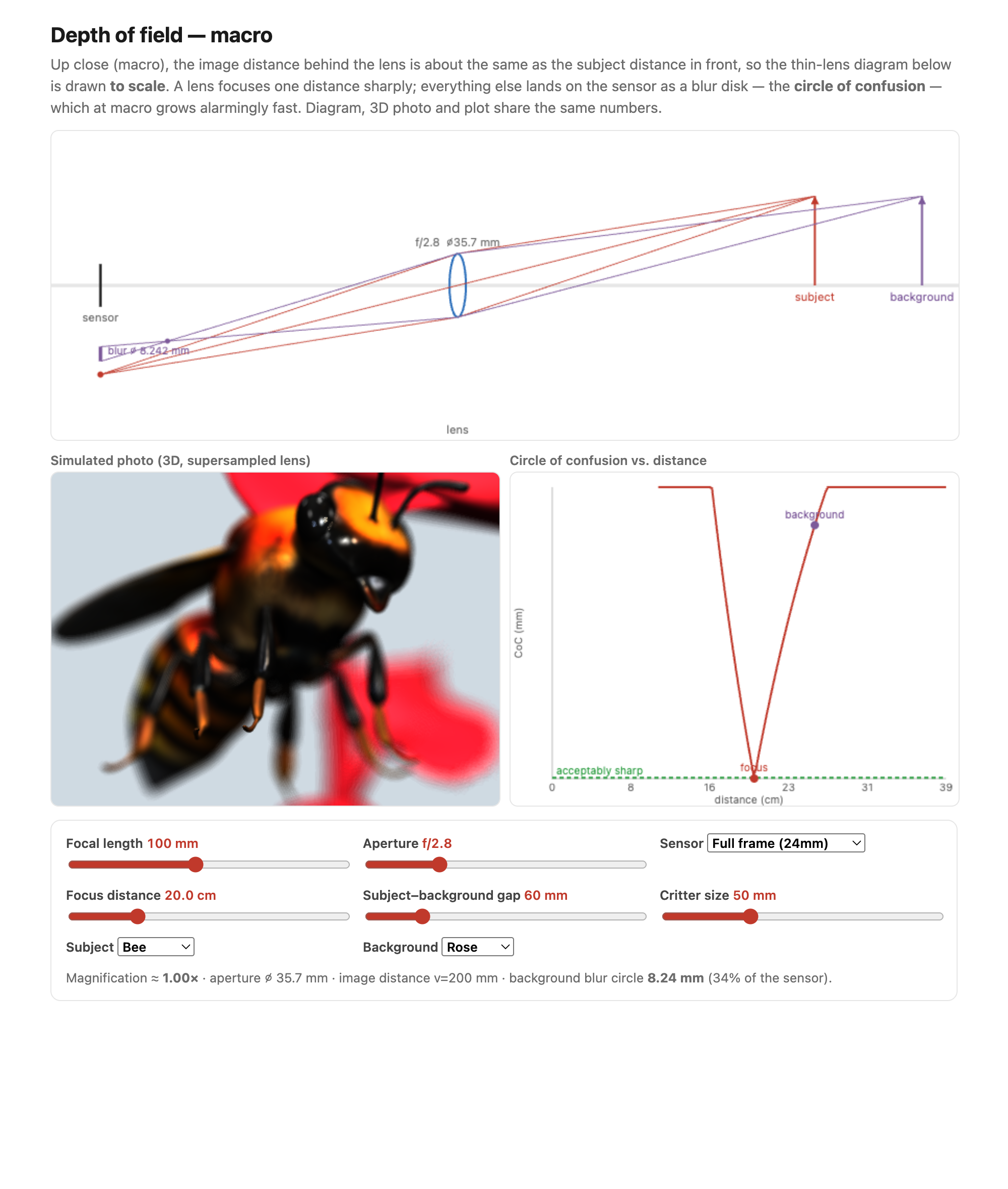
• **defocus / focus** — depth-from-defocus and focal stacks → [[Advanced computational photography#Light field and multi-aperture imaging]], Depth of field

• **dual-pixel** — the half-aperture parallax phones already capture for autofocus, reused for portrait depth → Optics (dual-pixel AF)

• **motion** — structure-from-motion / optical-flow parallax → [[Matching pixels across space and time]]

• **monocular cues** — a *single* still already implies depth to a human (occlusion, perspective, texture gradient, shading, familiar size, haze); turning those into numbers is the next chapter

• the recurring catch: most reconstructions recover geometry only **up to a similarity** (scale/rotation/translation) unless something fixes the **absolute scale** — a known baseline, a calibration target, or a metric sensor. Keep "relative" vs "metric" depth distinct.

• a deliberately reflective close (slides 84–86): the field is a **complex landscape** along several axes — *reconstruction* (output 3-D) vs *NVS* (output 2-D); *overfit-per-scene* (NeRF, 3DGS) vs *amortized* (DUSt3R, VGGT); *baked illumination* vs *relightable*; **number of input views** (1 → 360° → ∞); the **3-D representation** used (volumetric/fuzzy vs hard surface vs 4-D ray space — or none); how much **prior** is learned; world-space vs camera-space.

• the provocation worth leaving the reader with: the **Bitter Lesson** (Sutton) and the **"parable of the parser"** — when data + compute are plentiful, the hand-built intermediate (here, *explicit 3-D*) may be an unnecessary **"fake task"** that learning can skip. **Is 3-D still needed, or is it scaffolding we'll discard?** (Counterpoint: real applications — robotics, AR, fabrication, autonomous driving — keep wanting *actual* geometry. → [[Adjacent fields and applications]].)

• frontier (slide 50): scalability / long context, beyond shape+texture (materials, **relightability**), **motion** (dynamic scenes), less supervision, fewer inductive biases.

• the *output* counterpart to all of the above — once you have a 3-D scene, how do you *show* it with parallax? Brief pointer, since the optics live with light fields: **lenticular / parallax-barrier** autostereoscopic displays, **light-field displays**, head-tracked & VR/AR stereo, and research like **Project Starline**. Cross-link to the light-field display material in [[Advanced computational photography#Light field and multi-aperture imaging]] (lenticular displays, 3-D TV) rather than re-deriving.