BookNotesSlidesP-sets Syllabusdraft · v0.2.49.1
💬Comments welcome. To leave a note, select any text and click the note / highlight button that pops up — or open the panel with the tab at the top-right (‹). Notes are visible only inside our private review group.
Computational Photography, an AI-powered Slopendium — 21 Inpainting
expand to📖 Full book outline1 parts · 4 chapters · 20 sections · 9 figures embedded · 3 placeholders · double-click a figure to enlarge
▸Part 21 INPAINTING⧉
<!--uid: inpainting-->
▸21.1 Inpainting, texture synthesis, and object removal⧉
fig-inpaint-prior-spectrum
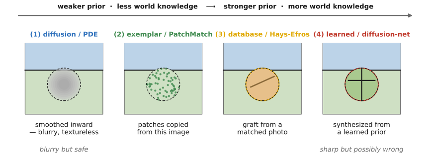
fig-inpaint-prior-spectrum · the hole-filling prior spectrum: PDE/diffusion (smoothness) → exemplar/texture (self-similarity) → learned/generative (semantics) 🟨
fig-pde-isophote-diffusion
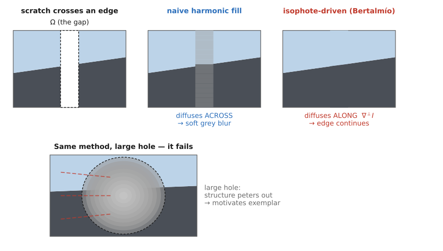
fig-pde-isophote-diffusion · PDE inpainting continues isophotes (level lines) smoothly into the hole — diffusion of structure inward (Bertalmío 2000) 🟨
fig-thin-lens-vs-real
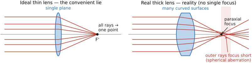
fig-thin-lens-vs-real · side-by-side "convenient lie vs reality": ideal thin lens (single plane, all parallel rays → one focus) vs a real thick multi-surface lens where outer rays focus short of the paraxial focus (spherical aberration → blur, no single point) ✅
fig-efros-leung-growth
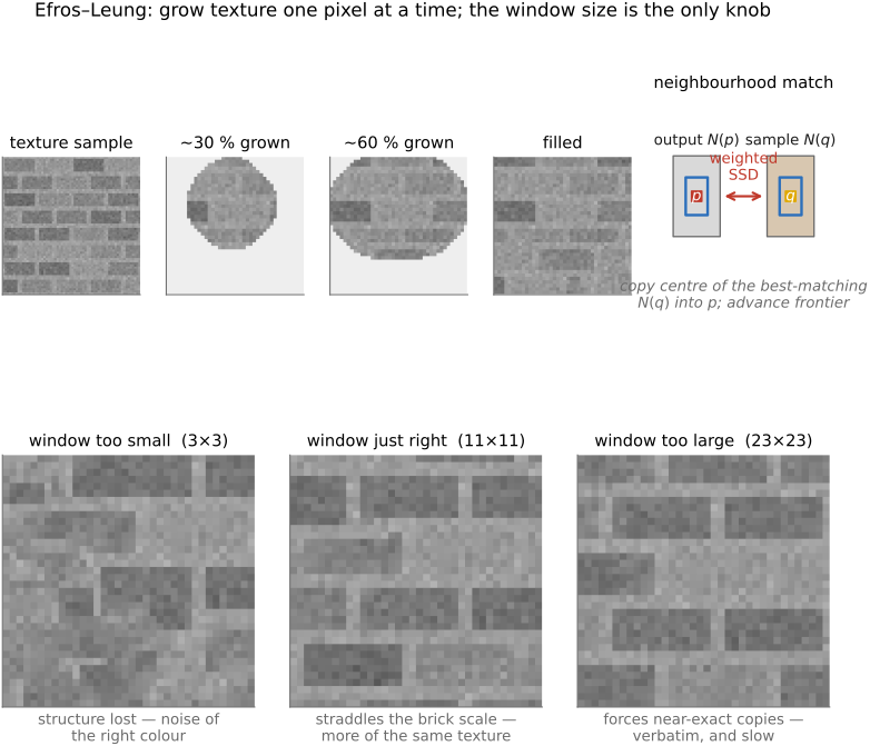
fig-efros-leung-growth · Efros–Leung non-parametric synthesis: grow one pixel at a time by matching its known neighborhood against the sample 🟨
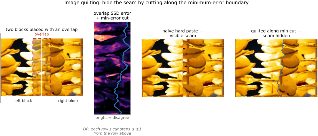
fig-quilting-seam
fig-quilting-seam · image quilting: lay overlapping patches and cut along the minimum-error boundary so seams disappear (Efros–Freeman 2001) 🟨
⬜ figure not yet created
`fig-object-removal` (Criminisi: a person erased, the hole filled by confidence-/edge-priority patch order so structures continue across it) fig-object-removal
⬜ figure not yet created
`fig-highlight-recovery` (a clipped specular spot → inpainted plausible surface color) fig-highlight-recovery
This chapter is the most literal instance of 💡 L10. A hole has **no measurement at all** — the only thing that can fill it is a model of what images look like. So inpainting is best read as a **ladder of priors**, from the weakest ("be smooth") to the strongest (a learned generative model), and the whole chapter is *which prior, and where it copies-vs-invents*. The recurring honesty: filled pixels are **plausible, never measured** — verifiable when the prior copies genuine structure from elsewhere, an outright **guess** when it hallucinates.
💡 **Big lesson (recurrence of L5.4 · the prior is not optional):** filling a hole is the purest case — there is *zero* data inside it, so **100% of the answer comes from the prior.** Smoothness, self-similarity, a photo database, a learned net — each is a different prior, and the result is exactly as good (and as honest) as the prior is. (→ see Big lesson **L5.4**, first placed in [[#Super-resolution]]; here taken to its extreme — no data, all prior.)
▸21.2 Patch match⧉
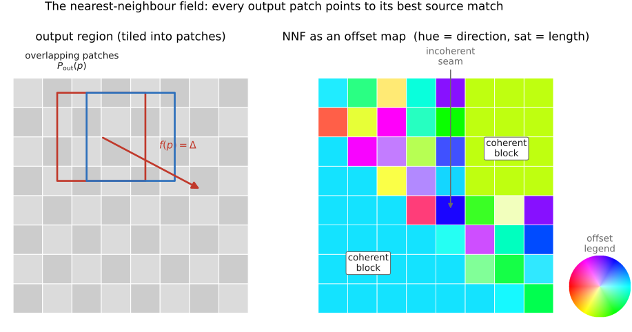
fig-nnf-field
fig-nnf-field · the nearest-neighbor field: every patch points to its best match elsewhere — visualized as a color-coded offset map 🟨
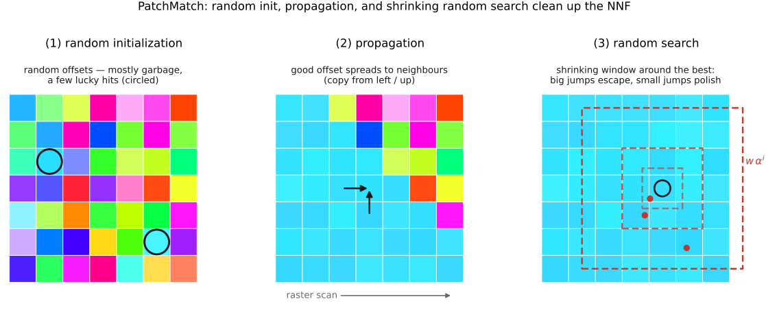
fig-patchmatch-three-steps
fig-patchmatch-three-steps · PatchMatch's three moves — random initialisation → propagation (good offsets spread to neighbors) → random search (refine locally) 🟨
⬜ figure not yet created
`fig-patchmatch-apps` (one image → hole-filled, retargeted (wider, no distortion), reshuffled (an object dragged, surround re-synthesized)) fig-patchmatch-apps
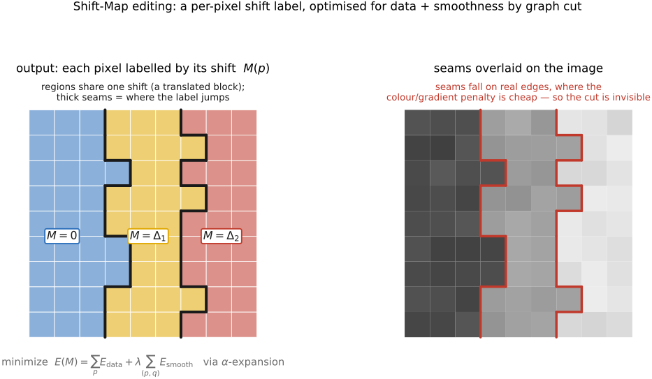
fig-shiftmap-labeling
fig-shiftmap-labeling · Shift-Map editing as a graph-cut labeling: each output pixel is assigned a shift, optimized for data + smoothness 🟨
The previous chapter's exemplar methods (Efros–Leung, Criminisi) all live or die on one operation: *for each patch, find its most similar patch elsewhere.* Done naively that's a full search per patch — far too slow to be interactive, and the real reason texture synthesis felt like a batch job. This chapter is the **two ways to make that fast or optimal**: a brilliant **randomized heuristic** (PatchMatch) that gets a near-perfect answer in milliseconds, and a **global graph-cut** (Shift-Map) that gets the *optimal* answer more slowly. The unifying object is the **nearest-neighbor field**; the unifying lesson is 💡 **L6.4** — *the edit is an optimization over a correspondence, and the energy you pick is the design.*
💡 **Big lesson (recurrence of L6.4 · image edits as optimization on a graph):** "where does each output pixel come from?" is a **labeling** — assign every output pixel a **shift** into the input. Pick the **energy** — a data term (respect the user's keep/remove/resize constraints) plus a **seam** term (neighboring pixels should take consistent offsets, so cuts fall on real edges) — and a generic **graph-cut** solver does the rest. PatchMatch is the *fast heuristic* answer to the same labeling; Shift-Map is the *globally-optimal* one. (→ see Big lesson **L6.4**, first placed in Seam optimization; it is the affinity lesson L4.21 turned into a *cut*.)
▸21.3 Inpainting using millions of photographs⧉
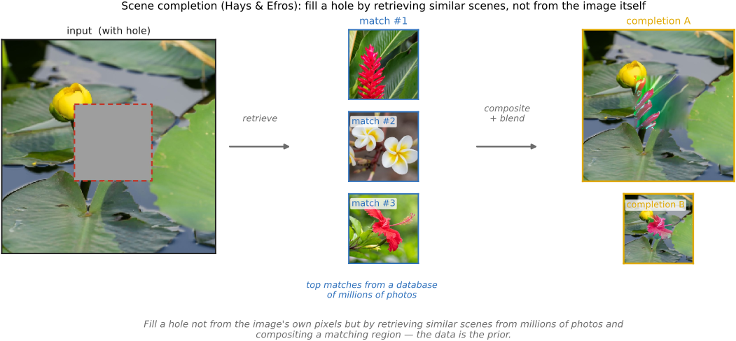
fig-scene-completion
fig-scene-completion · Hays & Efros scene completion: an image with a hole → top matching scenes retrieved from a database → plausible composited completions, Poisson-blended (Inpainting Using Millions of Photographs, 11.5) ✅
Hays and Efros's *Scene Completion* makes a startling bet: the best way to fill a hole in your photo is to find someone else's photo of a similar place and copy its pixels in. Where classical inpainting hallucinates from the image's own texture, this retrieves from a corpus of millions and lets the *data* be the prior — and it works precisely because, at that scale, a matching scene almost always exists. It is the ancestor of every "millions of photographs" method in this part, and the clean foil to model-based diffusion inpainting.
▸21.4 Generative inpainting⧉