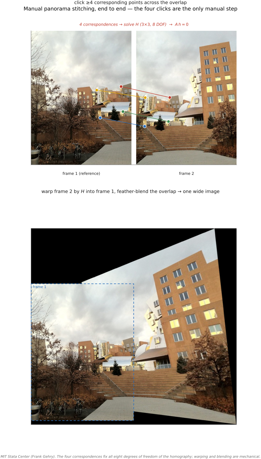
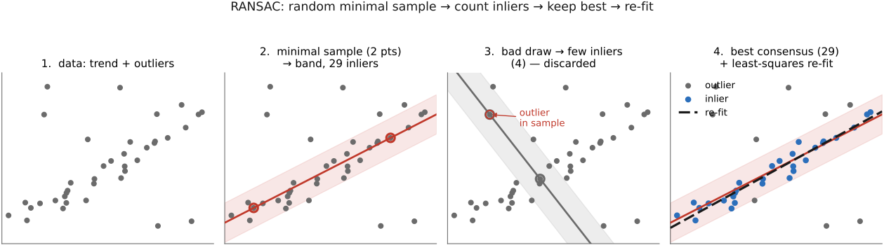
• **the setup**: we have point correspondences, most good (inliers) but some wrong (**outliers**), and we want the homography $H$. A plain **least-squares** fit over *all* matches is hopeless — even a few gross outliers drag the fit arbitrarily far off (squared error rewards them). We need a **robust** estimator. [`fig-ransac-pano-inliers`]
• **RANSAC** (RANdom SAmple Consensus, Fischler & Bolles 1981) — the loop:
1. **randomly pick a minimal sample** — for a homography, **4 correspondences** ($s=4$);
2. **fit the model exactly** from that sample (solve $H$);
3. **count inliers** — all matches with **small reprojection error** $\lVert\mathbf{x}_i'-H\mathbf{x}_i\rVert<\varepsilon$;
4. **keep the sample with the largest consensus set** (most inliers);
5. after the loop, **re-fit $H$ by least squares on all inliers** (optionally reweighted to pull in near-inliers). [`fig-ransac-line` shows the loop on a toy line fit; `fig-ransac-pano-inliers` on a real overlap]
• *pseudocode*: the canonical robust-fitting loop as a fence — sample 4, fit, count inliers, keep best, re-fit on inliers.
• **the intuition**: a model fit to an **all-inlier** sample is approximately correct and so will be **endorsed by many other inliers**; a model contaminated by an outlier is wrong and gets **few votes**. Consensus, not least squares, identifies the good model. The minimal sample size keeps the chance of a clean draw as high as possible.
• **probabilistic analysis — how many iterations?** Let $w$ be the **fraction of inliers** and $s$ the sample size. The probability a single random sample is **all inliers** is $w^s$ (independent draws → product / AND). The probability that $N$ samples **all fail** to be clean is $(1-w^s)^N$ (each independent → product). To **succeed with probability $p$**, demand $(1-w^s)^N \le 1-p$, giving
$$N \;=\; \frac{\log(1-p)}{\log(1-w^s)}.$$
[`fig-ransac-iterations-graph`]
• **read the three knobs** (state the takeaways):
• **sample size $s$ / model complexity** — the **bad** exponential: $w^s$ shrinks fast as $s$ grows (homography needs $s=4$, so $w^4$). More parameters → many more iterations.
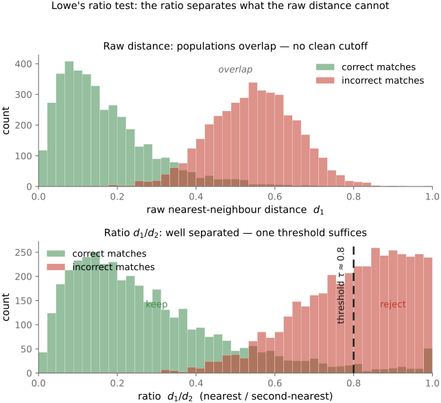
• **inlier fraction $w$** — the **base** of the exponential: cleaner matches → dramatically fewer iterations. (This is why the **ratio test runs first** — it *raises $w$*.)
• **iterations $N$** — the **good** exponential: failure probability falls geometrically with $N$, so a few extra iterations buy enormous reliability.
• **worked numbers** (from the slides, to ground it): with $s=4$ — at $w=0.5$, $w^s=0.0625$, so $N=100$ → fail prob $\approx0.0016$ (1 in 600), $N=1000$ → 1 in $10^{28}$. At $w=0.3$, $N=100$ → fail $\approx0.44$, $N=1000$ → 1 in 3400. At $w=0.1$, you need $\sim10^5$ iterations to be safe. **Inlier fraction dominates.**
• **the bigger lesson**: RANSAC is a **general robust-fitting** tool (lines, fundamental matrices, planes, …) — *fit a low-parameter model from a random minimal sample, score by consensus, keep the best, re-fit on inliers.* Cheap when the model needs few points and inliers aren't too rare.
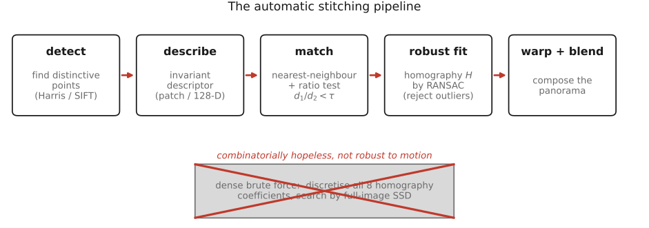
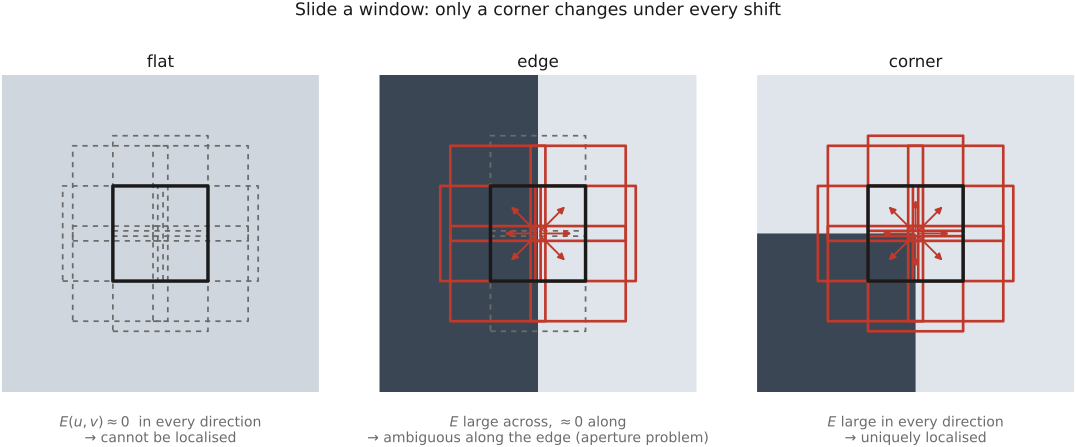
• **closing the loop — the whole auto-pano system**: extract **Harris** (or SIFT) interest points → describe (normalized patch / SIFT) → match by descriptor distance → **ratio test** rejects ambiguous matches → **RANSAC** fits the homography robustly → warp every image to the reference → **[[#Blending|blend]]**. That is automatic panorama stitching (Brown & Lowe 2007), and the same feature pipeline scales up to **bundle adjustment** ([[#Bundle adjustment]]) and full 3D reconstruction.