Computational Photography, an AI-powered Slopendium

▸Part 11 WARPING, MORPHING, AND LAGRANGIAN APPROACHES⧉

💡 **Big lesson (L17 · transport half):** almost every geometric technique is **(1) establish a correspondence / coordinate map**, then **(2) transport pixels along it** by warping and resampling. This part owns step (2) — one shared engine serving rectification, panoramas, morphing, stabilization, and frame interpolation — and the ways to *build* a map from sparse control. The hard *estimation* half (step 1) is [[Matching pixels across space and time]].

▸11.1 Warping⧉

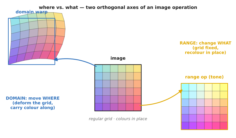
`fig-warp-domain-vs-range` · one image, two orthogonal arrows — the domain arrow bends the grid (a pixel slides, carrying its color; a warp), the range arrow recolours in place (a point/tone op); warping moves where, not what 🟨

⬜ figure not yet created

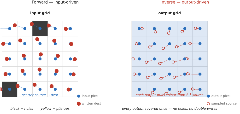
`fig-forward-warp-holes` (forward/input-driven warp scatters input pixels to fractional output locations → gaps (uncovered output) and pile-ups (many inputs to one output)) fig-forward-warp-holes

`fig-inverse-warp-lookup` · inverse (output-driven) warping, the useful idiom — loop over output pixels, push each back through $f^{-1}$, sample there; every output covered once, the only difficulty a clean resampling 🟨

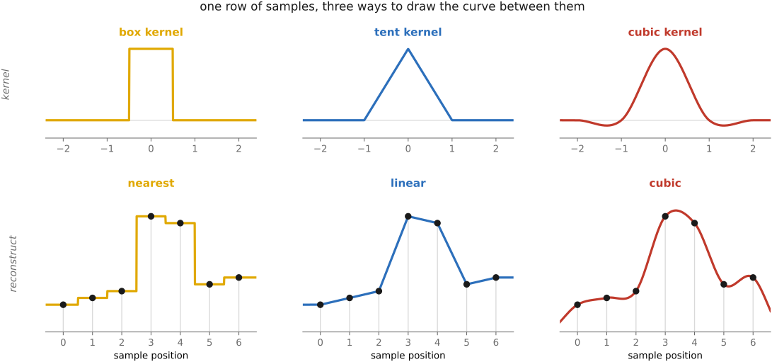
`fig-recon-filters-1d` · nearest (boxy staircase), linear (kinked through every sample), and cubic (smooth with mild overshoot) reconstruction of the same 1-D sample row — the sharpness/smoothness trade 🟨

⬜ figure not yet created

`fig-bilinear-weights` (the four surrounding pixels and the fractional-coordinate area weights of bilinear interpolation) fig-bilinear-weights

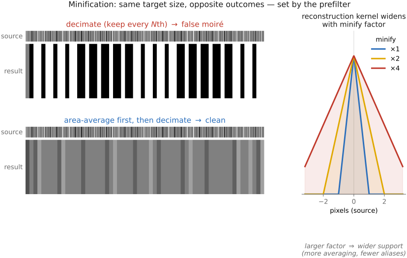
`fig-minify-aliasing-moire` · the L16 picture — a fine grating decimated naively (folds into false moiré) vs area-averaged first then decimated (clean); same size, opposite outcomes, decided by prefiltering 🟨

⬜ figure not yet created

`fig-kernel-scaling-minify` (the reconstruction kernel widened by the downscale factor so it averages over the right footprint — "gather farther when shrinking") fig-kernel-scaling-minify

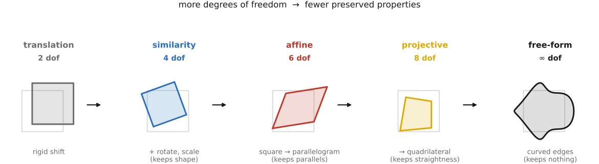
`fig-dof-ladder` · the degrees-of-freedom ladder — a unit square under translation (2) → similarity (4) → affine (6) → projective (8) → free-form ($\infty$), each rung breaking a preserved property 🟨

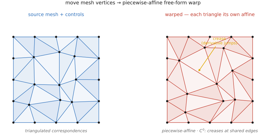
`fig-mesh-triangulation-warp` · piecewise-affine mesh warp — control matches triangulated, each triangle carrying its own affine map; exact and fast but only $C^0$, creasing along shared edges 🟨

⬜ figure not yet created

`fig-tps-rbf-warp` (a few control points displaced → a smooth thin-plate-spline field filling the gaps, minimal bending) fig-tps-rbf-warp

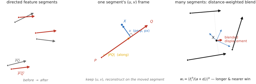
`fig-beier-neely-segments` · Beier–Neely feature-line warp — before/after directed segments, one segment's $(u,v)$ frame, and the distance-weighted blend of several segments' proposed displacements ($w_i=(\ell_i^p/(a+d_i))^b$) 🟨

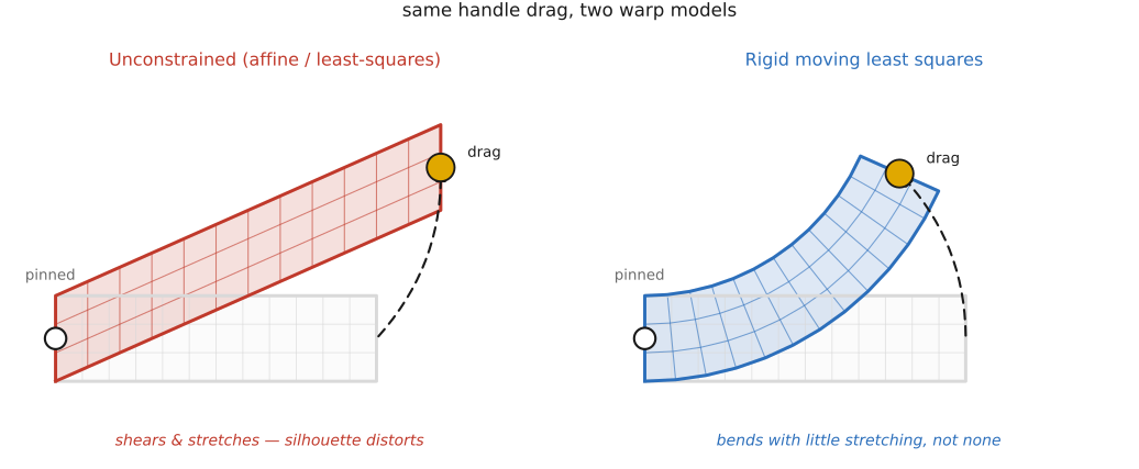
`fig-arap-vs-affine` · drag one handle — an unconstrained affine/least-squares warp shears and stretches, vs an as-rigid-as-possible / MLS warp that keeps each neighborhood near a rotation so the shape bends without stretching ✅

💡 **Big lesson (L16 · Prefilter before you downsample):** a warp that *shrinks* the image (minifies) is throwing samples away — and if you just decimate (keep every $N$th source pixel, or sample a narrow reconstruction kernel) the detail too fine for the new grid **folds down into bold false moiré**, not into nothing. The fix is to **area-average first**: widen the resampling kernel in proportion to the downscale factor $s$ (so it gathers over the whole footprint each output pixel now covers) and renormalize — that low-pass blur is the prefilter. Enlarging needs *no* prefilter (clamp the kernel width to 1); shrinking *always* does. (→ see Big lesson **L16**, first placed in BASIC → Resampling; the frequency-domain *why* is **L4.8** — aliasing folds frequencies above the new Nyquist. The same lesson governs every geometric resample in this part: rectification corners that shrink, stabilization crops, optical-flow rendering.)

⚠️ **Candidate new part-spine lesson (flag only — not registered).** Almost every algorithm in this part follows one shape: **establish a correspondence / coordinate map between two images (or an image and a target frame), then transport pixels along it.** Warping makes the map explicit and applies it; perspective rectification *solves* the map (a homography) from constraints; panorama stitching *estimates* the map from features; morphing *interpolates between* two maps; optical flow *estimates a dense map* from brightness constancy; stabilization *smooths a map over time*; frame interpolation *renders along* a map. A lesson like **"find the coordinate map, then move the pixels"** would unify the part the way L5.4 unifies the inverse-problem part. Worth registering as a part-spine lesson for MOTION/WARPING — *noted here, deliberately not registered* (registry-first convention: register in [[Big Lessons]] before placing).

equations

warp as a domain map $\text{out}(x,y)=\text{in}\big(f^{-1}(x,y)\big)$ (move the domain, keep the range)

**forward** warp $\text{out}(f(x,y))\leftarrow \text{in}(x,y)$ (scatters → holes)

1-D **linear** reconstruction $\text{im}(x)= (1-\alpha)\,\text{im}[\lfloor x\rfloor]+\alpha\,\text{im}[\lceil x\rceil]$, $\alpha=x-\lfloor x\rfloor$

**bilinear** = separable 1-D linear in $x$ then $y$ (four-neighbor area weights)

general **convolution resampling** $\text{out}(x)=\sum_{x'}k\big(f^{-1}(x)-x'\big)\,\text{in}(x')$ with analytic kernel $k$ centered at the fractional source location

**minification kernel scaling** $k_s(t)=\tfrac1s\,k(t/s)$ for downscale factor $s$ (widen + renormalize → area-average = prefilter, **L16**)

**affine** $\begin{psmallmatrix}x'\\y'\end{psmallmatrix}=A\begin{psmallmatrix}x\\y\end{psmallmatrix}+\mathbf t$ (6 DOF)

**projective / homography** $\begin{psmallmatrix}x'\\y'\\w'\end{psmallmatrix}=H\begin{psmallmatrix}x\\y\\1\end{psmallmatrix}$, then $(x'/w',y'/w')$ (8 DOF

solve from 4 correspondences — [[Manual panorama stitching from multiple views]])

**TPS / RBF** field $f(\mathbf p)=A\mathbf p+\mathbf t+\sum_i w_i\,\phi(\lVert\mathbf p-\mathbf c_i\rVert)$ with $\phi(r)=r^2\log r$ (thin-plate radial basis)

**Beier–Neely** single-segment map via the segment frame $u=\dfrac{(\mathbf X-\mathbf P)\cdot(\mathbf Q-\mathbf P)}{\lVert\mathbf Q-\mathbf P\rVert^2},\ v=\dfrac{(\mathbf X-\mathbf P)\cdot\perp(\mathbf Q-\mathbf P)}{\lVert\mathbf Q-\mathbf P\rVert}$, then $\mathbf X'=\mathbf P'+u(\mathbf Q'-\mathbf P')+\dfrac{v\,\perp(\mathbf Q'-\mathbf P')}{\lVert\mathbf Q'-\mathbf P'\rVert}$, multi-segment weight $w_i=\Big(\dfrac{\ell_i^{p}}{a+d_i}\Big)^{b}$.

▸11.1.1 Warping is a domain transform — move *where*, not *what*⧉

• **the one-line definition**: a warp applies a function $f:\mathbb{R}^2\to\mathbb{R}^2$ to the image *domain* — "if $(x,y)$ had color $c$ in the input, then $f(x,y)$ has color $c$ in the output." It deforms **where pixels live**, leaving their **colors (the range) untouched**. Contrast a *point/tone operation*, which edits the range (colors) and leaves the domain fixed. Warping is the domain twin of everything in BASIC point-ops. [`fig-warp-domain-vs-range`]

• **the rubber-sheet picture**: imagine the image printed on rubber and stretched — pixels slide to new positions; the picture content rides along. This is the right mental model for *all* of it, from a tiny lens-distortion correction to "liquify"/slimming, to morphing, to a full perspective rectification.

• **why it's everywhere** (motivate before machinery): geometric tasks across this whole part are warps — **optical aberration / lens-distortion correction**, **video stabilization**, **panorama reprojection** (fix parallax / align to a reference), **wide-angle distortion correction**, **morphable face models**, **image-based rendering**, and the cosmetic "slim the subject." One primitive, reused everywhere — which is exactly why this chapter comes first in the part.

• **two-and-a-half hard questions** (the chapter's skeleton, stated up front): given the rubber-sheet idea, three things are genuinely non-trivial — (1) *which direction* do we transform (forward or inverse)? (2) *how do we read a color at a non-integer location* (resampling/reconstruction)? and (2.5, only for free-form warps) *how do we even specify $f$* from a handful of user inputs? The next three sections take these in turn.

▸11.1.2 Forward vs inverse warping — why output-driven wins⧉

• **forward warp (input-driven)**: loop over every *input* pixel $(x,y)$, compute its destination $f(x,y)$, and write its color there: $\text{out}(f(x,y))\leftarrow\text{in}(x,y)$. Intuitive — "push each pixel to where it goes." But it has **two failure modes** baked in. [`fig-forward-warp-holes`]

• **holes / gaps**: destinations $f(x,y)$ are generally **non-integer** and **non-surjective** — when the warp stretches a region, neighboring inputs land far apart, leaving output pixels that **no input ever writes** (black speckle / cracks).

• **pile-ups / double-writes**: where the warp compresses a region, **many** inputs land on the **same** output pixel — who wins? You'd have to splat-and-accumulate with weights and normalize, which is fiddly and still doesn't fill the gaps.

• **inverse warp (output-driven)** — *the useful one*: loop over every *output* pixel $(x,y)$, push it **backward** through $f^{-1}$ to find where it came from in the input, and **look up** that color: $\text{out}(x,y)=\text{in}\big(f^{-1}(x,y)\big)$. [`fig-inverse-warp-lookup`]

• **why it wins**: the main loop is over **output** pixels, so **every output is covered exactly once** — no gaps, no double-writes by construction. The non-integer problem is pushed entirely into the *input* lookup, where it's a clean **resampling** question (next section) rather than a scatter problem.

• **take-home (state it as a rule)**: *main loop over OUTPUT pixels; use the INVERSE transform; resample the input.* This is the canonical resampling/warping idiom and recurs verbatim in panorama warping ([[Manual panorama stitching from multiple views]]) and rectification.

• **pseudocode**: a three-line block (loop output pixels → `(x',y')=f⁻¹(x,y)` → `out[x,y]=resample(in,x',y')`) makes the output-driven loop and once-per-pixel coverage concrete.

• **the catch — you need $f^{-1}$**: inverse warping needs the *backward* map. For **parametric** warps this is free (invert a matrix; for a homography, use $H^{-1}$). For a warp you only know **forwards** — most importantly a **dense optical-flow field** (each input pixel's motion) — you don't have $f^{-1}$ in closed form, and either invert the field numerically or fall back to forward splatting. So forward warping isn't *wrong*, it's the tool when the field is only available input-side. (Cross-ref [[Optical flow]] — rendering a frame along an estimated flow is exactly this case.)

• **boundary handling**: $f^{-1}(x,y)$ can land **outside** the input. Decide the policy — **black/zero padding**, **clamp-to-edge** (replicate the border pixel), **mirror**, or **mark as undefined** (transparent / alpha). Rectification and stabilization both produce outputs that read past the input border (the corners), so this is not a corner case — it's the common case.

11.1.3 Resampling — a quick reminder (developed in BASIC)⧉

▸11.1.4 Resampling — reading a value at a non-integer location⧉

• **the core problem**: inverse warping asks for $\text{in}$ at a **fractional** coordinate $f^{-1}(x,y)$. An image is *samples* of an underlying continuous signal; to read between samples we **reconstruct** the continuous signal and evaluate it — this is *resampling* (reconstruct, then re-sample). The reconstruction filter is the whole story.

• **nearest neighbor**: round to the closest sample. Cheapest; **blocky / jaggy** (a box reconstruction kernel) — visible stair-steps under rotation/scaling. Fine only for label maps / when you must not invent in-between values. [`fig-recon-filters-1d`, "nearest"]

• **bilinear**: linear interpolation in 1-D, $\text{im}(x)=(1-\alpha)\,\text{im}[\lfloor x\rfloor]+\alpha\,\text{im}[\lceil x\rceil]$ with $\alpha$ the fractional part; in 2-D it's **separable** — interpolate along $x$ on the two top and two bottom neighbors, then along $y$ (or $y$ then $x$ — same result, a worthwhile exercise). Equivalently the four-neighbor **area weights**. Smooth, cheap, the workhorse default; slightly soft (a triangle/tent kernel attenuates high frequencies). [`fig-bilinear-weights`]

• **bicubic / Lanczos** — *the right framing*: do **not** think "fit a cubic to the data." Think **convolution with an analytic kernel**: $\text{out}(x)=\sum_{x'}k\big(f^{-1}(x)-x'\big)\,\text{in}(x')$, the kernel $k$ centered at the (fractional) source location and sampled at the surrounding integer inputs. **Bicubic** (the Mitchell–Netravali family) uses a wider, sharper, negative-lobed kernel over a $4\times4$ neighborhood — sharper than bilinear, with slight ringing/overshoot you can tune. **Lanczos** is a windowed sinc, sharpest of the common kernels (more ringing). All are **separable** (run in $x$, then $y$), and in general the weights **can't be precomputed** because the fractional offset differs per output pixel (though for integer or rational scale factors they become periodic and *can* be tabulated). [`fig-recon-filters-1d`]

• **upsampling vs downsampling is the key split** (lead-in to L16): the kernel-as-convolution view makes the difference precise. **Upsampling (enlarging)**: reconstruct and read — clamp the kernel width to 1 input pixel; *no* prefilter needed (you're not discarding anything). **Downsampling (minifying)**: you're **discarding** samples, so reconstruction alone **aliases**.

• 💡 **the L16 discipline** — *prefilter before you downsample* (see the boxed lesson above): blur/area-average **before** decimating. In the convolution-resampling view this is one clean move: **scale the kernel up by the downscale factor**, $k_s(t)=\tfrac1s\,k(t/s)$, and renormalize — now each output pixel **gathers over the whole footprint** it covers in the input, i.e. averages instead of point-sampling. The infamous bug is **keep-every-Nth decimation** (or a width-1 kernel on minify): fine detail folds into bold **moiré / herringbone**. The honest rule: *upsampling clamps the kernel to width 1; downsampling widens it proportionally to scale.* [`fig-minify-aliasing-moire`, `fig-kernel-scaling-minify`]

• **practical notes**: resampling is **separable** — scale/resample in $x$ (producing an anisotropically-sized intermediate image), then in $y$; downsampling-in-$y$-first vectorizes well. Implementation-wise the clean trick (Adams) is to **form the tiny sparse 1-D resampling matrix** (one row/column's worth of weights, with boundary handling and renormalization folded in) and apply it to every row/column — the weight matrix is negligible next to the image. **For minification, MIP-maps** (a prefiltered pyramid) precompute the area-averages once and read them back per query — the standard real-time answer to L16. (Cross-ref [[Linearity, Fourier, Aliasing and deblurring]] for the Nyquist/aliasing account; pyramids for the band structure.)

• **the honest limit of interpolation** (forward-ref): resampling adds *pixels*, never new *frequencies* — bicubic/Lanczos upsampling looks soft because the high frequencies were never measured. Recovering plausible detail is **super-resolution**, a prior-driven inverse problem, not resampling (cross-ref [[What can super-resolution actually do?]] — reconstruction vs hallucination).

▸11.1.5 Specifying the warp I — parametric models and the degrees-of-freedom (DOF) ladder⧉

• **the idea**: for many warps $f$ is a **low-parameter** function — fit it to a few correspondences and apply it everywhere. Climbing the **degrees-of-freedom ladder**, each rung adds freedom and **breaks a preserved property**: [`fig-dof-ladder`]

• **translation** (2 DOF) — preserves everything but position.

• **rigid / Euclidean** (3) — + rotation; preserves lengths & angles.

• **similarity** (4) — + uniform scale; preserves angles & ratios (shape).

• **affine** (6) — $\binom{x'}{y'}=A\binom{x}{y}+\mathbf t$; preserves **parallelism** and **ratios along lines**, *not* angles/lengths. Straight lines stay straight; a square → a parallelogram.

• **projective / homography** (8) — $\binom{x'}{y'}{w'}=H\binom{x}{y}{1}$ then divide by $w'$; preserves **straight lines only** — parallels may **converge** (a square → an arbitrary quadrilateral). This is the rung that does **perspective**, and the subject of the next chapter and of panorama stitching.

• **why homogeneous coordinates** (link, don't re-derive): the homography is non-linear in $(x,y)$ because of the **division by $w'$**, but **linear** in homogeneous coordinates — a single $3\times3$ matrix multiply followed by the perspective divide. It *is* the reprojection of a plane under a 3-D rotation (project, rotate, reproject), which is why "depth doesn't matter for a planar-or-rotation warp." Full development: FUNDAMENTALS — Pinhole; the **solve** for $H$ from correspondences: [[Manual panorama stitching from multiple views]].

• **fitting a parametric warp**: each point correspondence gives **two equations**; an affine needs **3** correspondences (6 unknowns), a homography **4** (8 unknowns up to scale). More correspondences → **overdetermined** → **least squares** (or SVD for the homography null-vector). This is a clean instance of [[Image formation as a linear system]] — *the warp parameters are the regression unknowns.* (Robustness to wrong matches → RANSAC, developed for stitching.)

• **strength and limit**: parametric warps are **global, smooth, few-parameter, robust** — perfect when the deformation really is rigid/affine/projective (a plane, a camera rotation, a lens model). They **cannot** express a local, free-form deformation — a smile, a morph, a hand-drawn stretch. For that, you need a field built from sparse control (next).

▸11.1.6 Specifying the warp II — free-form warps from sparse correspondences⧉

• **the setup**: the user gives a **sparse** set of correspondences — a few control points, or pairs of feature segments — and we must produce a **dense** warp field $f$ defined at every pixel by *interpolating* the sparse constraints. Three standard constructions, trading smoothness, locality, and control:

• **mesh / triangulation warp (piecewise-affine)**: triangulate the control points (e.g. Delaunay); inside each triangle the three vertex correspondences **exactly determine an affine map** (6 DOF, 3 points), so warp each triangle by its own affine. Simple, fast, exact at the controls, and the standard morphing workhorse. Downside: **$C^0$ only** — the field is continuous but **creases** at triangle edges (derivative jumps), and quality depends on the triangulation. [`fig-mesh-triangulation-warp`]

• **RBF / thin-plate-spline (TPS) warp (smooth scattered-data interpolation)**: fit a **smooth** field that interpolates the control displacements with **minimal bending energy**: $f(\mathbf p)=A\mathbf p+\mathbf t+\sum_i w_i\,\phi(\lVert\mathbf p-\mathbf c_i\rVert)$, an affine "global" part plus a sum of **radial basis functions** centered at the controls. The thin-plate kernel $\phi(r)=r^2\log r$ minimizes integrated second-derivative energy — the smoothest interpolant (the physical analogy: a thin metal plate bent to pass through the constraints). The weights $w_i$ (and $A,\mathbf t$) solve a small **linear system**. Smooth everywhere ($C^1$+), no creases; **global support** (every control influences every pixel, so it can be less local than a mesh) and an $O(n^2)$–$O(n^3)$ solve in the number of controls. The go-to for smooth medical/face registration and morphometrics (Bookstein). [`fig-tps-rbf-warp`]

• **feature-based field warping — Beier & Neely 1992**: specify the warp with **pairs of directed line segments** (before/after) rather than points — natural for features like an eyebrow or a jawline. Each segment pair $(\mathbf{PQ}\to\mathbf{P'Q'})$ defines a **local coordinate frame**: a coordinate $u$ **along** the segment (normalized, $0$ at $\mathbf P$, $1$ at $\mathbf Q$) and $v$ **perpendicular** (in distance units). For a single segment, map a point by reading its $(u,v)$ in the **destination** segment's frame (inverse warp) and reconstructing it in the source frame:

• $u=\dfrac{(\mathbf X-\mathbf P)\cdot(\mathbf Q-\mathbf P)}{\lVert\mathbf Q-\mathbf P\rVert^2}$, $\quad v=\dfrac{(\mathbf X-\mathbf P)\cdot\perp(\mathbf Q-\mathbf P)}{\lVert\mathbf Q-\mathbf P\rVert}$; then $\mathbf X'=\mathbf P'+u\,(\mathbf Q'-\mathbf P')+\dfrac{v\,\perp(\mathbf Q'-\mathbf P')}{\lVert\mathbf Q'-\mathbf P'\rVert}$.

• **note** (Beier–Neely's own finding): $u$ scales with the segment (stretch), but $v$ is kept **absolute** — they tried scaling $v$ too and it looked worse.

• **multiple segments**: each segment $i$ proposes a displaced point $\mathbf X'_i$; the result is a **distance-weighted average**, weight $w_i=\big(\ell_i^{\,p}/(a+d_i)\big)^{b}$ — longer segments ($\ell_i$) carry more influence, nearer ones ($d_i$ = distance to the segment) dominate; $a,b,p$ tune the falloff. [`fig-beier-neely-segments`]

• **provenance / use**: the technique behind Michael Jackson's *Black or White* morph; a classic course problem set. *Built here, used in [[Morphing]].* (Ref: Beier & Neely 1992; the canonical warping text is Wolberg 1990.)

• **as-rigid-as-possible (ARAP) / MLS warps — penalize shear**: the catch with the above is that interpolating positions alone lets shapes **shear and squash** unnaturally when you drag a handle. **As-rigid-as-possible** (Igarashi 2005) and **moving-least-squares** rigid/similarity deformation (Schaefer 2006) add an explicit objective: each local neighborhood should transform **as close to a rotation+translation (rigid) as possible** — minimize the deviation from rigidity rather than just matching control points. The deformation then **preserves local shape** (a dragged limb bends but doesn't stretch), which is what makes interactive shape manipulation and detail-preserving warps look natural. Conceptually: same "dense field from sparse handles," but with a **regularizer on local rigidity** instead of plain smoothness. [`fig-arap-vs-affine`]

• **choosing** (decision aid): a **plane / camera rotation / lens model** → parametric (affine/homography), fit by least squares. A **face/shape morph** with creases acceptable and speed wanted → **mesh/triangulation**. A **smooth** registration with few controls → **TPS/RBF**. **Feature-line** control (eyebrows, jaw) → **Beier–Neely**. **Interactive handle-dragging** where shapes must not shear → **ARAP/MLS**. Whatever the choice, the *application* is identical: produce $f$, then **inverse-warp and resample** (the first three sections) — that primitive never changes.

11.1.7 Liquify: brush-driven warping⧉

11.1.8 Liquify — the warp with a paintbrush bolted on⧉

▸11.2 Antialiasing for complex transforms⧉

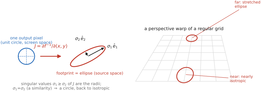
`fig-footprint-ellipse-jacobian` · one output-pixel circle back-projected through a perspective warp maps to a footprint ellipse; major/minor axes = singular values/vectors of the local Jacobian J (square only under a similarity); + a worked perspective grid ✅

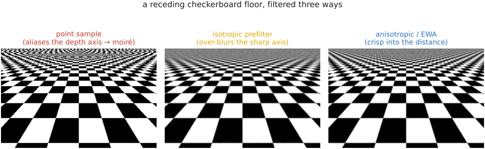
`fig-isotropic-vs-anisotropic-floor` · receding checkerboard floor filtered three ways: point (aliased moiré) / isotropic (over-blur) / anisotropic-EWA (crisp into distance) ✅

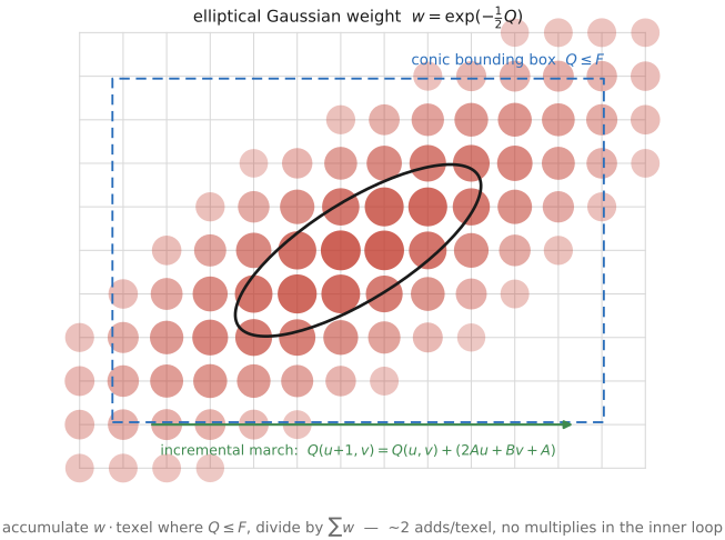
`fig-ewa-gaussian-ellipse` · elliptical-Gaussian EWA weight over source texels; conic Q≤F bounding box; incremental finite-difference march ✅

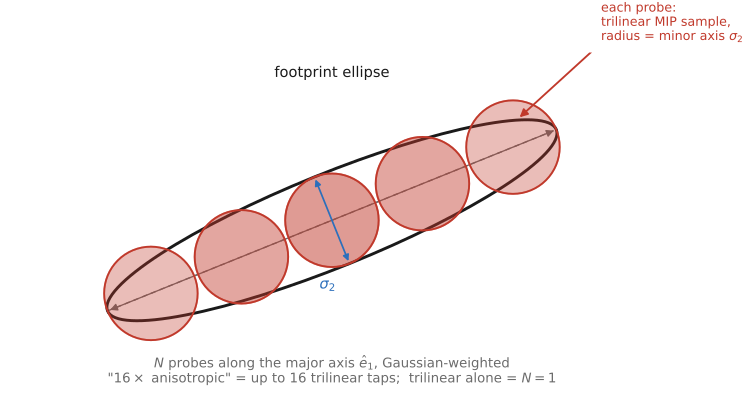
`fig-feline-probe-line` · footprint ellipse approximated by a line of N circular trilinear MIP probes along the major axis, each sized to the minor axis (16× anisotropic; trilinear = N=1) ✅

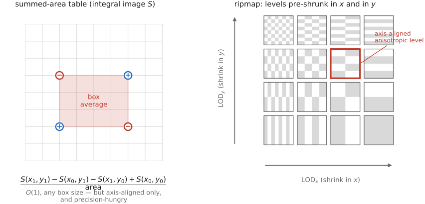
`fig-sat-ripmap` · summed-area table box average from 4 corner lookups of the integral image + ripmap grid of pre-shrunk-in-x/-in-y levels (axis-aligned anisotropy only) ✅

💡 **Big lesson (L16, anisotropic):** the prefilter-on-minify discipline (**L16**) is *direction-dependent* the moment the warp stops being a similarity. A general warp compresses the source more along one axis than another, so the right prefilter is not a round blur but an **oriented ellipse** — average a lot along the compressed direction, barely at all across it. Isotropic filtering must then either alias the compressed axis or blur the sharp one; anisotropic filtering (EWA and its approximations) does both jobs at once. Same lesson, one dimension richer.

equations

**footprint Jacobian** $J=\partial f^{-1}/\partial(x,y)$ (local linearization of the inverse warp)

the unit screen circle → ellipse with **covariance** $\Sigma=JJ^{\!\top}$, radii the singular values $\sigma_1\ge\sigma_2$ of $J$, **anisotropy** $\rho=\sigma_1/\sigma_2$

**EWA conic / Mahalanobis form** $Q(\mathbf u)=\mathbf u^{\!\top}\Sigma^{-1}\mathbf u=Au^2+Buv+Cv^2$, weight $w=\exp(-\tfrac12 Q)$ for $Q\le F$ (an elliptical Gaussian)

**incremental evaluation** $Q(u{+}1,v)=Q(u,v)+(2Au+Bv+A)$ with the increment itself stepped by the constant $2A$ → ~2 adds/texel

**Feline** probe centers $\mathbf c_i=\mathbf c\pm t_i\,\hat{\mathbf e}_1$ along the major axis $\hat{\mathbf e}_1$, each a trilinear sample at level $\text{LOD}=\log_2\sigma_2$, Gaussian-weighted

**summed-area box** average $=\big(S(x_1,y_1)-S(x_0,y_1)-S(x_1,y_0)+S(x_0,y_0)\big)/\text{area}$ with $S$ the integral image

**max-anisotropy clamp** $\sigma_1\leftarrow\min(\sigma_1,\rho_{\max}\sigma_2)$.

▸11.2.1 When the footprint stops being a square — the warp Jacobian⧉

• **the setup**: inverse warping reads $\text{in}$ at $f^{-1}(x,y)$ ([[Warping]]). But an output pixel is not a *point* — it is a little area, and what we owe it is the **average of the source over the region that maps into it**. Under a *uniform* scale that region is a square and the isotropic L16 kernel is right. Under a general warp it is not.

• **the footprint is an ellipse**: linearize the inverse warp about the pixel — its **Jacobian** $J=\partial f^{-1}/\partial(x,y)$ — and the unit screen circle (one output pixel) maps to an **ellipse** in source space, the *footprint*. Its shape is read straight off $J$: the **singular values** $\sigma_1\ge\sigma_2$ are the major/minor radii, the **singular vectors** their directions. A *similarity* (uniform scale + rotation) has $\sigma_1=\sigma_2$ — a circle, back to isotropic. Anything else ($\sigma_1>\sigma_2$) is genuinely anisotropic. [`fig-footprint-ellipse-jacobian`]

• **the canonical offender — the receding plane**: a checkerboard floor rendered in perspective (or rectified *to* perspective). Near the camera one pixel covers one tile; toward the horizon one pixel covers *many tiles in depth but only one across* — a long thin ellipse, anisotropy $\rho=\sigma_1/\sigma_2$ in the tens or hundreds. This is where every isotropic filter visibly fails. [`fig-isotropic-vs-anisotropic-floor`]

• **why isotropic can't win**: a round filter sized to the *minor* axis leaves the major axis under-filtered → **aliasing / shimmer** along the depth direction; sized to the *major* axis it over-filters the minor → **blur** across it. One radius cannot serve two very different extents. The fix is to make the kernel an ellipse that matches the footprint. (This is exactly the L16 prefilter, now with an orientation.)

▸11.2.2 EWA — the elliptical weighted average⧉

• **the idea** ([@greene-heckbert-1986|Greene & Heckbert 1986]; the full account is [@heckbert-1989|Heckbert's 1989 thesis]): weight each source texel inside the footprint by an **elliptical Gaussian** matched to the ellipse, and normalize. It is the gold-standard anisotropic prefilter — the reconstruction-and-prefilter convolution of [[Warping]] with the kernel finally allowed to be non-round.

• **the conic makes it cheap to test**: the ellipse is the level set of a quadratic, the **Mahalanobis form** $Q(\mathbf u)=\mathbf u^{\!\top}\Sigma^{-1}\mathbf u=Au^2+Buv+Cv^2$ with $\Sigma=JJ^{\top}$ the footprint covariance; a texel is inside when $Q\le F$ and its weight is $\exp(-\tfrac12 Q)$. So filtering is: walk the ellipse's bounding box, accumulate $w\cdot\text{texel}$ where $Q\le F$, divide by $\sum w$. [`fig-ewa-gaussian-ellipse`]

• **the incremental trick** (Heckbert): $Q$ is a quadratic in integer texel coordinates, so along a scanline $Q(u{+}1,v)-Q(u,v)=2Au+Bv+A$ is *linear*, and *its* increment is the **constant** $2A$. Stepping two running sums turns the per-texel cost into ~2 additions and a table lookup for $\exp$ — no multiplies in the inner loop. Elegant, and the reason EWA was practical in 1986.

• **the cost and its cap**: work is proportional to the **ellipse area** $\sim\sigma_1\sigma_2$, which explodes at grazing angles. The standard guard is a **max-anisotropy clamp** $\sigma_1\leftarrow\min(\sigma_1,\rho_{\max}\sigma_2)$ (and a minor-axis floor of one texel): beyond the cap you accept a little extra blur rather than an unbounded sample count. EWA is usually run *on a MIP pyramid* too — pick the level where the minor axis is ~1 texel, then the ellipse spans only a handful of texels at that level.

▸11.2.3 Feline and anisotropic MIP probing — EWA on a GPU budget⧉

• **the move** ([@mccormack-etal-1999|McCormack, Perry, Farkas & Pijewski 1999], *Feline* = Fast Elliptical Lines): don't integrate the whole ellipse — **approximate it by a line of circular probes** strung along the major axis. Each probe is an ordinary **trilinear MIP sample** sized to the *minor* axis (so it averages correctly *across* the ellipse), and the $N$ probes spaced along the major axis cover its length; sum them with Gaussian weights. [`fig-feline-probe-line`]

• **this is what "16× anisotropic" means**: hardware anisotropic filtering is exactly this — $N$ (up to 16) trilinear taps along the footprint's long axis. **Trilinear alone** (Williams' MIP-map, [@williams-1983]) is the $N{=}1$ degenerate case: one isotropic probe that must pick a single LOD for both axes and therefore over-blurs the sharp one. Feline restores the lost axis at a few× the cost, not the ellipse-area cost of full EWA.

• **the trade-off**: more probes → closer to true EWA, more bandwidth; capped by $\rho_{\max}$ (the "max anisotropy" slider). The minor-axis-sized trilinear tap reuses the prefiltered pyramid, so each probe is $O(1)$ — the whole appeal.

▸11.2.4 Other footprint integrators — summed-area tables and ripmaps⧉

• **summed-area tables** ([@crow-1984|Crow 1984]): precompute the **integral image** $S$; then the average over any *axis-aligned* box is **four corner lookups** $\big(S(x_1,y_1)-S(x_0,y_1)-S(x_1,y_0)+S(x_0,y_0)\big)/\text{area}$ — $O(1)$, *any* box size, no pyramid. The catches: it handles **axis-aligned rectangles only** (no rotation → still not a true ellipse), and the partial sums grow huge, so it is **precision-hungry** (wide integer / float storage). [`fig-sat-ripmap`]

• **ripmaps**: an anisotropic MIP-map — separately pre-shrunk in $x$ and in $y$, a 2-D grid of levels $(\text{LOD}_x,\text{LOD}_y)$ — so an **axis-aligned** anisotropic footprint reads one level directly. Still blind to *rotation*, and 4× the storage of a MIP-map.

• **where each sits**: SAT and ripmaps buy **axis-aligned** anisotropy cheaply; EWA and Feline buy **arbitrarily-oriented** anisotropy (the receding-floor case), which is the one that actually arises under perspective. In practice GPUs ship Feline-style probing; SATs live on in integral-image tricks (box filters, Viola–Jones, local contrast) more than in texturing.

▸11.2.5 Footprint estimation, clamping, and when to reach for it⧉

• **estimating $J$**: in a renderer the Jacobian comes free from screen-space derivatives of the texture coordinates ($\partial u/\partial x$ etc., the GPU's `ddx`/`ddy`); in an image warp it is the local linearization of $f^{-1}$ you already evaluate. Two derivative vectors → the $2\times2$ $J$ → $\Sigma=JJ^{\top}$ → the ellipse. (For minification with *no* warp, $\Sigma$ is a circle of the downscale radius and EWA degenerates back to the isotropic L16 prefilter — the chapters are continuous.)

• **clamping for stability**: cap $\rho$ at $\rho_{\max}$ (bound the work / probe count); floor the minor radius at one texel (never sample below the base level); be careful at **silhouettes and discontinuities**, where the linearization lies and a clamped, slightly-blurred answer beats a sharp wrong one.

• **decision aid (when is this worth it?)**: a gentle affine, a panorama warp, a mild lens correction → the **isotropic** L16 prefilter (a MIP-map + trilinear) is plenty. Reach for **EWA / Feline** only under **strong perspective, swirls, or grazing minification** — anywhere the footprint ellipse gets genuinely long and one axis would otherwise alias. That is precisely the rectifier's non-uniform Jacobian ([[Perspective distortion and its correction]]) and the receding-ground case.

• **forward-ref — EWA splatting**: the *same* elliptical Gaussian runs in reverse for point-based rendering — [@zwicker-etal-2002|Zwicker et al.'s EWA splatting] *forward*-splats each point as an elliptical Gaussian footprint into the image, the antialiasing dual of EWA texture filtering and a direct ancestor of today's Gaussian-splatting view synthesis. (Cross-ref the novel-view-synthesis material.)

11.2.6 Jacobians of common warps⧉

▸11.3 Morphing⧉

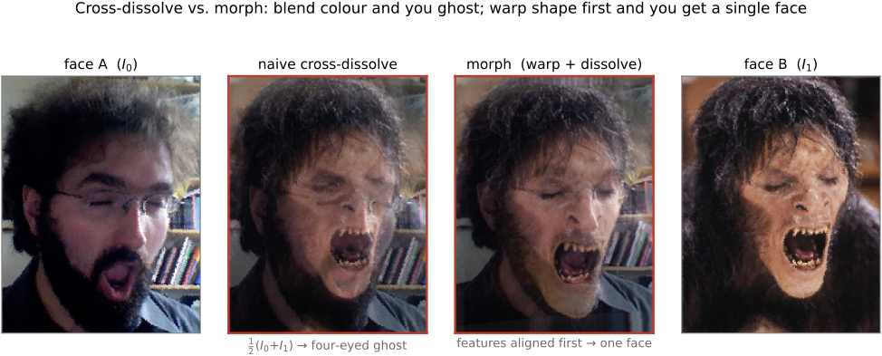
`fig-morph-crossfade-ghost` · why a cross-dissolve ghosts — two misaligned faces averaged at $t=0.5$ superimpose features into a translucent four-eyed, two-mouthed ghost; the blend handled color but ignored position ✅

⬜ figure not yet created

the failure that motivates everything)

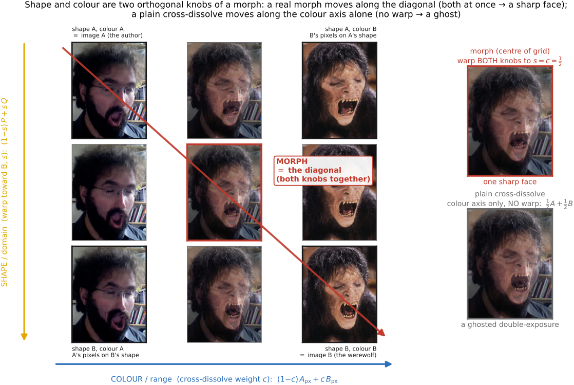
`fig-morph-shape-vs-color` · the two orthogonal knobs of a morph — range (color) as the cross-dissolve and domain (shape) as feature-position interpolation; a true morph is their product, the square's corners labeling the four extremes 🟨

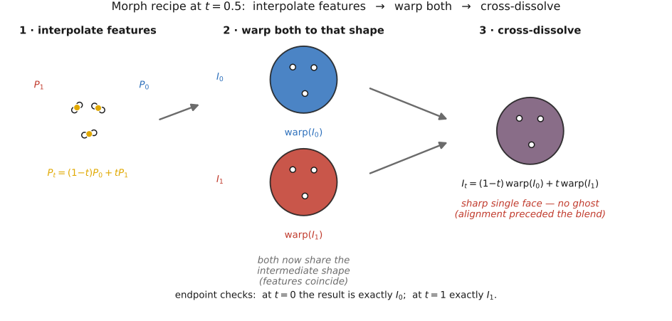
`fig-morph-recipe` · the three-step morph at $t=0.5$ — interpolate the features to the midpoint shape, warp both images to that same shape, then cross-dissolve; a sharp single face because alignment preceded the blend 🟨

⬜ figure not yet created

`fig-beier-neely-oneseg` (a single before/after line pair: the $(u,v)$ coordinate frame along/perpendicular to the segment, and how a point $X$ maps to $X'$) fig-beier-neely-oneseg

⬜ figure not yet created

`fig-beier-neely-multiseg` (several line pairs, each proposing an $X'_i$, combined by a distance/length **weighted average** — the field warp) fig-beier-neely-multiseg

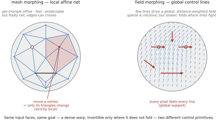
`fig-mesh-vs-field-morph` · two ways to drive the same morph — mesh (per-triangle affine, strictly local, fiddly, can crease) vs field/Beier–Neely (a few control lines, globally-supported distance-weighted field, sparse but fold-prone) 🟨

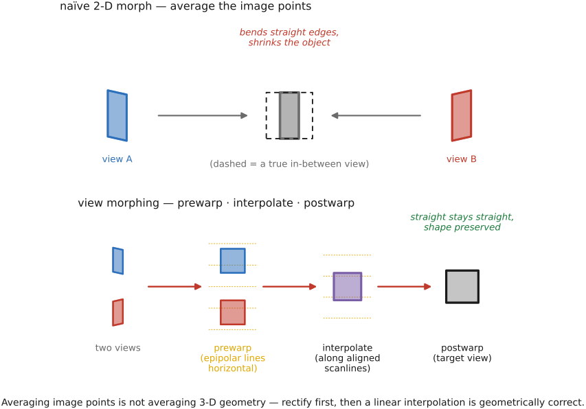
`fig-view-morph-prewarp` · why two views need view morphing — a naive 2-D morph bends straight edges and shrinks a rotating object, vs view morphing (prewarp to aligned epipolar lines → interpolate → postwarp) keeping lines straight and shape intact 🟨

💡 **Big lesson (recurrence — *align before you blend*):** averaging two images only makes sense once their features sit at the *same place*. A plain cross-dissolve blends colors at fixed coordinates, so any misalignment **double-exposes into a ghost**; the cure is to **warp into correspondence first, then average** — the same move as panorama de-ghosting and multi-frame super-resolution's sub-pixel alignment. Morphing is this lesson taken to its limit: not just align-then-average, but interpolate the *alignment itself* over $t$. (Companion to the *capture-then-decide / align-then-merge* family; the dense automatic aligner is [[Optical flow]].)

▸11.3.1 Why a cross-dissolve isn't enough — the ghosting motivation⧉

• **the goal**: *smoothly* turn one image into another — a face into another face, one video keyframe into the next (slow-motion / frame interpolation). "Smooth" means the in-between $I_t$ should look like a *plausible single image*, not a blend of two.

• **the naive attempt — cross-fading (a.k.a. cross-dissolve)**: linearly interpolate colors pixel-by-pixel, $\;\text{out}[y,x] = (1-t)\,I_0[y,x] + t\,I_1[y,x]$. This is the right idea for **color** but ignores **position**.

• **why it ghosts**: the two images' **features are not aligned** — eyes, mouth, silhouette sit at different pixels. Blending colors at fixed locations super-imposes a left-image eye on a right-image cheek → a translucent **double exposure** (four eyes, two mouths). And you generally *cannot* fix this with one global alignment (translate/rotate/scale) — faces differ locally, non-rigidly. [`fig-morph-crossfade-ghost`]

• **the diagnosis**: cross-fading interpolates only the **range** (color). To get a believable in-between we must *also* interpolate the **domain** — the **location** of every feature. This is a **domain transform** (a warp), and it's the missing half.

• 💡 **the throughline**: *separate shape and color, and interpolate each.* Everything below is how to (a) get a dense **shape** interpolation from sparse correspondence and (b) combine it with the **color** interpolation. (See the *align before you blend* big-lesson box above.)

▸11.3.2 Two interpolations: domain (shape) and range (color)⧉

• **range interpolation (color)** — the cross-dissolve we already have: $\;C(x) = (1-t)\,C_0(x) + t\,C_1(x)$. A straight linear blend of pixel values.

• **domain interpolation (location)** — treat a feature **point** as a vector and interpolate *where it is*: for corresponding points $P$ (in $I_0$) and $Q$ (in $I_1$), the in-between location is $\;V = (1-t)\,P + t\,Q$. At $t=0$ the feature is where $I_0$ put it; at $t=1$ where $I_1$ put it; in between it travels along the straight segment. [`fig-morph-shape-vs-color`]

• **warping = a domain transform**: moving pixels spatially while leaving their colors alone, $\;C'(x,y) = C\big(f(x,y)\big)$. In practice we use the **inverse / backward** map — for each output pixel, look up where it came from: $\;\text{out}(x,y) = \text{im}\big(f^{-1}(x,y)\big)$ — so every output pixel is filled (no holes) and resampling is well-defined. This is exactly the engine of [[Warping]]; morphing is one of its biggest customers (it warps twice per frame).

• 💡 **the morph in one line**: *interpolate the domain like a vector, then interpolate the range (color).* A morph is the **product** of a shape interpolation and a color interpolation — two independent linear blends applied together. [`fig-morph-shape-vs-color`]

▸11.3.3 The morphing recipe (combine both)⧉

• **inputs**: two images $I_0$ and $I_1$, plus **sparse correspondences** the user specifies on both (matching line segments, or matching mesh vertices — *which* primitive is the next two sections). Output: a sequence of in-betweens $I_t$, $t\in(0,1)$.

• **per intermediate frame $I_t$** (the canonical four steps):

1. **interpolate the feature geometry** to an intermediate shape: each corresponding pair (point/segment/vertex) $\to$ its in-between location $P_t = (1-t)\,P_0 + t\,P_1$.

2. **build a dense warp field** from the sparse pairs — two of them: one taking $I_0$'s features onto the intermediate shape, one taking $I_1$'s features onto the *same* intermediate shape.

3. **warp both images** to that common shape. Now $I_0$ and $I_1$ are **feature-aligned**: both pairs of eyes land on the same pixels, both mouths coincide.

4. **cross-dissolve** the two warped images: $I_t = (1-t)\,\text{warp}(I_0) + t\,\text{warp}(I_1)$. Because they're aligned, the blend is sharp — **no ghosting**. [`fig-morph-recipe`]

• **why warp *both* (not just one)**: warping only $I_0$ all the way to $I_1$'s shape and dissolving would make features *slide* while colors fade — and would over-distort early/late frames. Meeting **in the middle** (both warp partway to the shared intermediate shape) keeps distortions small and symmetric, and is what makes the motion read as one object transforming.

• **endpoints check**: at $t=0$ the intermediate shape = $I_0$'s shape, warp of $I_0$ is identity, color weight on $I_1$ is 0 → output is exactly $I_0$ (and symmetrically at $t=1$). The morph is a *genuine* interpolation, not just a fancy blend.

• **note (cross-ref)**: the correspondences here are **user-specified and sparse**. The **automatic, dense** way to get correspondence between two images is [[Optical flow]] — that's exactly what frame-interpolation / slow-motion methods use to morph between *video* frames without hand-drawn lines ([[Frame interpolation and slow-motion synthesis]]).

▸11.3.4 Field morphing: the Beier–Neely line-pair warp⧉

• **the primitive**: a **pair of directed line segments** — one drawn on the "before" image, one on the "after" — saying *"this feature edge here corresponds to this feature edge there."* A handful of segments (jaw, eyes, nose bridge, hairline) is enough; the warp interpolates everywhere else. (Beier & Neely 1992 — "Feature-Based Metamorphosis"; the technique behind Michael Jackson's *Black or White* video and a classic pset.)

• **one segment defines a coordinate change**: a before/after pair $\overline{PQ}\to\overline{P'Q'}$ induces a similarity (rotate + scale + translate) — the simplest transform that carries one segment onto the other. Set up a **segment-relative coordinate system**: along the segment, a **normalized** coordinate $u\in[0,1]$ (0 at $P$, 1 at $Q$); perpendicular to it, a **signed distance** $v$ (in pixels). For a query point $X$:

$$u = \frac{(X-P)\cdot(Q-P)}{\lVert Q-P\rVert^2}, \qquad v = \frac{(X-P)\cdot \text{perp}(Q-P)}{\lVert Q-P\rVert},$$

where $\text{perp}(\cdot)$ is the 90°-rotated vector. Then the corresponding point in the *other* image is reconstructed from the *primed* segment:

$$X' = P' + u\,(Q'-P') + \frac{v\cdot\text{perp}(Q'-P')}{\lVert Q'-P'\rVert}.$$

Read it: **$u$ scales** with the segment (a feature twice as long stretches with it), but **$v$ stays in absolute pixel units** (perpendicular offset is *not* rescaled — Beier & Neely report that scaling $v$ too looked worse). [`fig-beier-neely-oneseg`]

• **inverse-map direction**: you compute $(u,v)$ in the **destination** ("after") frame and look up the source — because warping uses the **inverse** map ($\text{out}(x)=\text{im}(f^{-1}(x))$), so each output pixel is filled.

• **multiple segments → a weighted average of displacements**: each line pair $i$ proposes its own target $X'_i$. Combine them by a **distance-weighted average**, where a line's influence falls off with the query point's distance to that segment and grows with the segment's length:

$$X' = \frac{\sum_i w_i\,X'_i}{\sum_i w_i}, \qquad w_i = \left(\frac{\text{length}_i^{\,p}}{a + \text{dist}_i}\right)^{b}.$$

The tunables $a,b,p$ control smoothness ($a$: how strongly far lines still pull), falloff ($b$), and the length bias ($p$). Distance-to-a-segment is the usual capped point-to-segment distance (perpendicular within the span, endpoint distance outside). [`fig-beier-neely-multiseg`]

• **strengths / weaknesses**: *strength* — sparse, intuitive control (draw a few feature lines), smooth fields, no mesh to manage. *weakness* — every line affects every pixel (global support → $O(\#\text{pixels}\times\#\text{lines})$ per frame), and far-apart lines can fight, giving "ghost" pulls and folds; careful $a,b,p$ tuning and debugging the distance function are part of the work.

• **bells & whistles**: morph the **foreground only** (matte it first) so the background doesn't drag artifacts; **non-uniform** timing (different features morph at different rates) for more lifelike transitions.

▸11.3.5 Mesh / triangulation morphing (the alternative warp)⧉

• **the primitive**: instead of lines, place a **mesh of corresponding control points** on both images (or a regular grid deformed to match features). Triangulate the points; each triangle in $I_0$ maps to the matching triangle in $I_1$.

• **the warp**: within each triangle the map is a single **affine** (barycentric) transform — fast, local, and exactly invertible. The intermediate shape is the mesh with vertices at $P_t=(1-t)P_0+tP_1$; warp each source by its per-triangle affine onto that mesh, then dissolve. (Spline/free-form mesh variants — Wolberg 1990; multilevel free-form, Lee et al. 1996 — trade the piecewise-affine creases for smoother fields.)

• **field vs mesh — the trade**: *mesh* warps have **local support** (a vertex moves only its incident triangles → fast, predictable, no far-line fights) but the control net is fiddly and triangle edges can crease; *field (Beier–Neely)* warps have **global, line-based** control (sparse and intuitive) but are slower and can fold. Same job — *turn sparse correspondence into a dense, invertible warp* — two different bases. [`fig-mesh-vs-field-morph`]

• **either way, the same resampling**: each warp is a domain transform that must **reconstruct + prefilter** as it resamples (minified regions averaged, magnified regions smoothly interpolated) — the EWA/mip machinery of [[Warping]]. Morphing is a stress test for good resampling.

▸11.3.6 View morphing — the geometrically-correct in-between of two views⧉

• **when a 2-D morph is *wrong***: if $I_0$ and $I_1$ are two **photographs of the same 3-D scene** from different viewpoints (e.g. a face turning), a naive linear morph **bends straight lines and shrinks the object** — the in-between is not a valid view of *any* rigid scene. Linearly interpolating image positions is **not** the same as interpolating the underlying 3-D geometry. [`fig-view-morph-prewarp`]

• **the fix (Seitz & Dyer 1996, *View Morphing*)** — three steps that make the morph a *physically valid* intermediate view:

1. **prewarp** both images by homographies that **rectify** them to a common plane (so the two image planes are parallel and corresponding **epipolar lines** are horizontal and aligned);

2. **linearly interpolate** the now-rectified images (a plain morph — but in this rectified frame the linear interpolation *is* geometrically correct, because corresponding points move along aligned scanlines);

3. **postwarp** the result by an interpolated homography to the desired in-between view.

• **why it works**: rectification turns the general two-view geometry into the **parallel-camera (pure-translation) case**, where image-space linear interpolation exactly corresponds to moving the camera along the baseline — straight lines stay straight, the object keeps its shape, and the in-between is a true perspective view. It's the projectively-aware upgrade of the plain morph.

• **the connection to flow / stereo**: view morphing needs **corresponding points** between the views and the epipolar geometry relating them — exactly the **correspondence** problem of [[Optical flow]] and stereo, and the **epipolar** constraint of [[Brute force|Image alignment]] / multi-view. With dense correspondence you can synthesize in-between *views* automatically — the bridge from morphing to **image-based rendering** and to flow-driven **frame interpolation** ([[Frame interpolation and slow-motion synthesis]]).

▸11.3.7 Recap and significance⧉

• **the lasting ideas**: (1) **linear interpolation of color alone introduces blur/ghosts** — you must interpolate position too; (2) **separate shape and color**, then recombine; (3) **non-rigid alignment** of different images is a reusable primitive. [`fig-morph-recipe`]

• **where it goes**: **special effects** (the canonical face-morph); **video frame interpolation / slow-motion** and even **MPEG-style** motion prediction (morph-by-motion-field); **morphable models** for face recognition/animation (warp a mean face by shape parameters); **motion magnification** (Liu et al. 2005 — *analyze* a motion field, **magnify** it, and warp by the magnified field — a morph whose correspondence comes from motion analysis, robust to occlusion). The common thread: once you can **warp one image into correspondence with another**, you can interpolate, exaggerate, average, or re-render — and *getting* that correspondence automatically is the subject of the next chapter.

▸11.4 Morphable models⧉

11.4.1 Step 1 — dense correspondence: the precondition for averaging shapes⧉

11.4.2 Step 2 — Procrustes alignment: factor out pose so PCA sees shape⧉

11.4.3 Step 3 — PCA: a mean and a basis of eigen-deformations⧉

11.4.4 Step 4 — shape and appearance are *separate* bases⧉

11.4.5 Step 5 — fitting a new photo: analysis-by-synthesis⧉

11.4.6 Step 6 — once fitted, edit by moving in the space⧉

11.4.7 Step 7 — from linear PCA to neural priors⧉

11.4.8 Recap and significance⧉

▸11.5 Shape-preserving warping⧉

11.5.1 Why plain interpolation shears: the rigidity gap⧉

11.5.2 As-rigid-as-possible (ARAP) manipulation⧉

11.5.3 Linear blend skinning and why the weights decide everything⧉

11.5.4 Bounded biharmonic weights (BBW)⧉

11.5.5 ARAP interpolation: rigid-as-possible morphing between two poses⧉

11.5.6 Moving least squares: the simpler cousin⧉

11.5.7 Recap and significance⧉

▸11.6 Perspective distortion and its correction⧉

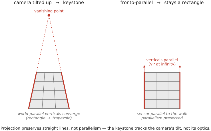
`fig-keystoning-cause` · keystoning is the tilt, not the lens — a camera tilted up makes world-parallel verticals converge (façade → trapezoid), while the fronto-parallel shot keeps them parallel; projection preserves lines, not parallelism 🟨

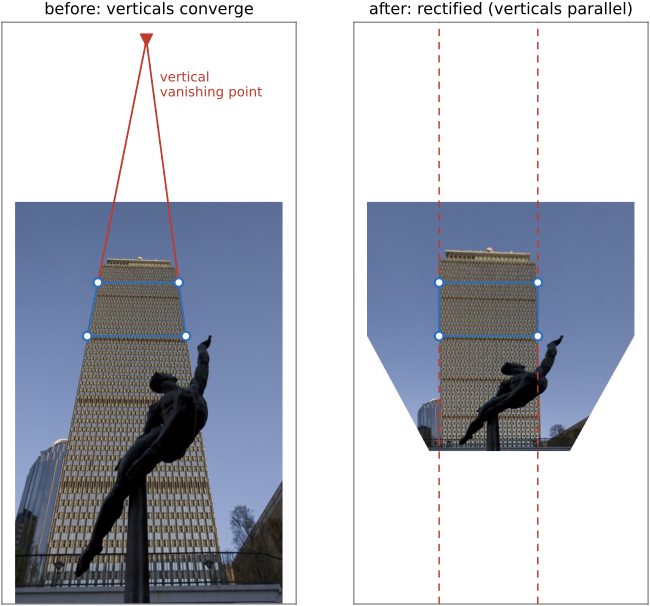
`fig-rectify-before-after` · rectifying by homography — a keystoned input with four corner handles dragged onto a known rectangle (vanishing point marked) re-rendered fronto-parallel by $\text{out}(\mathbf x)=\text{in}(H^{-1}\mathbf x)$ 🟨

⬜ figure not yet created

`fig-vanishing-point-autosolve` (detected parallel-line bundles meeting at vanishing points → the homography that sends the vertical VP to infinity straightens the verticals) fig-vanishing-point-autosolve

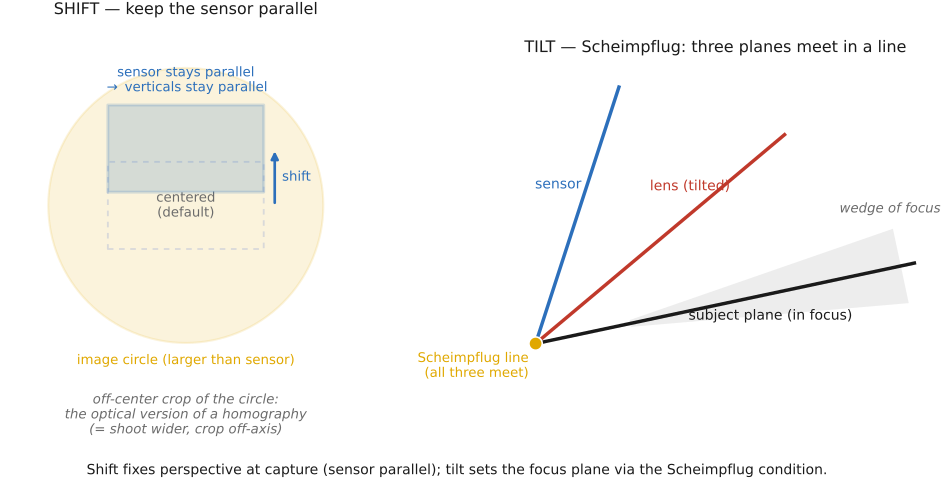
`fig-tilt-shift-scheimpflug` · fixing perspective in the lens — shift moves the sensor within an oversized image circle while staying parallel to the façade (no converging verticals), tilt sets the focus plane via the Scheimpflug condition 🟨

⬜ figure not yet created

`fig-rectify-resample-stretch` (the rectified output's non-uniform resolution: the far/top corners are enlarged and softened while the near edge is compressed — why one homography only rectifies a *plane*). fig-rectify-resample-stretch

💡 **Big lesson (L16 recurrence · prefilter the shrinking corners):** rectification does not resample uniformly — to make the *far* (top) of the façade as wide as the *near* edge, the homography **enlarges** the top corners (upsample → just interpolate) and **compresses** other regions (downsample → must prefilter, or alias). So a faithful rectifier applies the **prefilter-before-downsample** discipline *per region*, with the kernel footprint set by the **local Jacobian** of $H$ (how much each area shrinks). (→ see Big lesson **L16**, [[Warping]] / BASIC Resampling.)

equations

the rectifying map is a **homography** $\mathbf x' \simeq H\mathbf x$ (homogeneous

divide by $w'$) — the projective warp of [[Warping]]

solve $H$ from **4 correspondences** (building corners → target rectangle), each pair giving 2 linear equations, $H$ up to scale → 8 DOF (least squares / SVD, per [[Manual panorama stitching from multiple views]])

applied by **inverse warp + resample** $\text{out}(\mathbf x)=\text{in}\big(H^{-1}\mathbf x\big)$

the **auto** constraint: choose $H$ so the bundle of (imaged) parallel lines maps to a **vanishing point at infinity** (verticals become vertical / parallel).

▸11.6.1 Keystoning is projection, not a lens flaw⧉

• **the symptom**: aim the camera **up** at a tall building and its **parallel verticals converge** toward the top (keystoning); aim it down and they splay. Wide-angle shots show the same projective effect as exaggerated **near/far stretch** (the close part of a façade looms, the far part shrinks). Photographers find converging verticals **objectionable** in architecture — a building "looks more formal if the verticals stay vertical." [`fig-keystoning-cause`]

• **the cause** (the key reframing): this is **perspective projection doing its job**, not the lens misbehaving. Projection **preserves straight lines** but **does not preserve parallelism, angles, or lengths** — so a bundle of world-parallel verticals images as a bundle of lines **converging to a vanishing point**. (Contrast with *radial lens distortion* — barrel/pincushion — which **bends straight lines** and *is* an optical defect; that's a **different correction**, now developed in [[Slopendium/Compound lenses, and aberration correction]] (*Aberrations correction* — radial distortion correction). Keystoning bends nothing; lines stay straight, they just stop being parallel.)

• **faces in a wide-angle shot — the perceptual stake**: the same near/far stretch is what makes **faces** shot up close with a wide lens look wrong — the nose looms, the ears recede. There's no single plane to rectify (a face is 3-D), so the fix is **per-face / content-aware un-distortion** — locally re-warp each face region toward how it would have looked from farther away. What makes this worth doing is *perceptual*, not merely geometric: a face's perceived **shape — and even its perceived personality** (trustworthiness, competence, attractiveness) — **depends on the camera-to-subject distance**, which is the basis for correcting wide-angle portrait distortion (Perona 2007; perceived-trait-vs-distance study Bryan et al. PMC4114730). This is the same focal-length-vs-distance fact that governs portrait lenses — cross-ref [[Fundamentals]] (Lenses and focal length).

• **the giveaway**: if the **image plane is parallel to the subject plane** (sensor parallel to the façade), then world-parallel lines parallel to the sensor **stay parallel in the image** — no convergence. Convergence appears exactly when you **tilt** the sensor off the façade. So the distortion is a function of **camera orientation**, and that is precisely what a homography can undo.

▸11.6.2 The fix is a homography — re-render the façade fronto-parallel⧉

• **the idea**: the converging-verticals photo *is* a perspective image of a real planar rectangle (the façade). A **homography** maps between any two images of a plane — so there exists a single $3\times3$ projective warp $H$ that re-renders the façade **as if the sensor had been parallel to it**, sending the converging lines back to parallel. This is the **projective rung** of the DOF ladder from [[Warping]], applied here with the *target* being a fronto-parallel rectangle. [`fig-rectify-before-after`]

• **why one homography suffices (for a plane)**: reprojecting a plane = "project, rotate the camera, reproject," which is exactly a homography (depth drops out — *all points on the plane*, indeed all points along each ray, reproject identically). This is the same "depth doesn't matter for a planar-or-rotation warp" fact that makes panorama stitching work. **Cross-ref [[Manual panorama stitching from multiple views]]** — *identical machinery*; there the second image is another *view*, here it's the *target rectangle*.

• **solving $H$ — method 1, four corner correspondences**: pick **4 points** on the building (the corners of a known-rectangular feature — a window, the façade outline) and specify where they should go (a true rectangle, verticals vertical). 4 correspondences → 8 equations → solve the 8-DOF homography (up to scale) by **least squares / SVD**, exactly as in [[Manual panorama stitching from multiple views]]. This is the manual **perspective crop** in Photoshop. [`fig-rectify-before-after`, the 4 points]

• **solving $H$ — method 2, automatic via vanishing points**: detect bundles of **parallel lines** (the verticals, and the horizontals) — each images as a bundle meeting at a **vanishing point**. Choose the homography that sends the relevant vanishing point **to infinity** (making the verticals vertical/parallel again, and optionally the horizontals too). This needs **no user clicks** — it's the basis of Lightroom's **Upright** (it finds straight lines and squares them up) and of single-view metric rectification (Liebowitz & Zisserman 1998; Criminisi 2000). [`fig-vanishing-point-autosolve`]

• **applying it**: once $H$ is known, **inverse-warp and resample** — $\text{out}(\mathbf x)=\text{in}(H^{-1}\mathbf x)$, loop over output pixels, push back through $H^{-1}$, resample the input (the primitive from [[Warping]]). Same forward-vs-inverse and resampling care as everywhere.

• **in practice (tools)**: **Lightroom Transform / "Upright"** (auto and guided modes), **Photoshop perspective crop**, and dedicated architecture tools all do exactly this homography. The user experience is "drag the building straight"; the engine is the 4-point or vanishing-point homography.

▸11.6.3 The optical alternative at capture — tilt-shift / Scheimpflug⧉

• **fix it in the lens, not in post**: a **view camera** or **tilt-shift lens** corrects perspective **at capture**. The lens projects an image circle **larger than the sensor**; **shifting** the lens (or the sensor / back) selects an **off-center** part of that circle while keeping the **sensor parallel to the façade**. Because the sensor stays parallel to the subject plane, **verticals never converge** in the first place — no post-warp, no resampling penalty. [`fig-tilt-shift-scheimpflug`]

• **equivalent to "wider-angle + crop"**: a shift is geometrically the same as taking a **wider, centered** view and **cropping** to the off-axis region you want — which is also why software "perspective crop" can approximate it (at the cost of resolution). **Tilt** (the other view-camera movement) instead controls the **plane of focus** via the **Scheimpflug** condition (lens, sensor, and subject planes meet in a line) — used to get a slanted plane all-in-focus, or, reversed, the "miniature/tilt-shift" toy-town look. **Cross-ref Optics — Special optics** for the optical derivation; here we only note it as the at-capture counterpart of the homography. The two are related by — unsurprisingly — **a homography** (the shifted-sensor image and the tilted-sensor image of the same façade differ by a projective warp).

• **trade-off** (when to use which): optical correction **preserves resolution and avoids resampling artifacts** but needs special (expensive, manual) gear and must be decided **at capture**; the software homography is **free and deferrable** ("decide later") but **resamples** (next).

▸11.6.4 Cropping wide-angle photographs: recenter with a homography, don't just crop⧉

11.6.5 A different perspective distortion — wide-angle portraits, and a content-aware fix⧉

▸11.6.6 Beyond faces: correcting arbitrary objects (MaDCoW)⧉

11.6.7 A montage has no single viewpoint — a family in a box⧉

▸11.6.8 Recomposing perspective after capture: computational zoom⧉

▸11.6.9 The catch — resampling cost and "only a plane rectifies exactly"⧉

• **rectification resamples and stretches**: making the far/top of the façade as wide as the near edge means the homography **enlarges** some regions and **compresses** others → the output has **non-uniform resolution** (top corners enlarged and **softened**; other parts compressed). The enlarged regions are interpolation-limited (no new detail — cross-ref [[What can super-resolution actually do?]]); the compressed regions must be **prefiltered before downsampling** (**L16**, see the recurrence box) or they alias. The kernel footprint should follow the **local Jacobian** of $H$. [`fig-rectify-resample-stretch`]

• **you lose frame / pixels**: the rectified rectangle generally doesn't fill the original frame — corners read **outside** the input (boundary policy from [[Warping]]) and you usually **crop** to the valid region, sacrificing field of view and resolution. "Upright" with auto-crop is managing exactly this.

• **only a plane is exact** (the fundamental limit): a single homography exactly rectifies a **single plane**. A real 3-D scene (a building with depth, foreground objects, a receding street) has **multiple planes at different depths** — one homography can square up **one** of them, but everything off that plane is left distorted (and parallax between depths can't be removed by any 2-D warp). Genuinely correcting a 3-D scene needs **depth or multiple views** (image-based rendering / multi-view) — cross-ref view morphing and the panorama parallax caveat in [[Manual panorama stitching from multiple views]]. The honest scope of this chapter: **planar** perspective correction.

▸11.6.10 Where this sits — one map, then transport⧉

• **the single instance of the part spine (L17)**: this is the **simplest** member of the *establish a coordinate map, then transport the pixels along it* family — the map is **parametric** (one homography), the scene is a **single plane**, the input is **one image**. The map is *solved* (4 corners / vanishing points), not estimated.

• **closing link / where the family goes harder**: the next time the **same** homography machinery appears it aligns **two views** into a panorama ([[Manual panorama stitching from multiple views]], where the map must be *estimated* from feature matches); after that the maps become **dense and estimated** (optical flow) rather than parametric and solved. Same two steps throughout; only the map gets harder.

▸11.6.11 Robustness of perspective to the viewer's viewpoint⧉