• two chapters, one line. [[#Imaging as a linear system]] said a camera is a **linear projection**, $\mathbf{y}=A\mathbf{x}$; [[#Noise, signal-to-noise ratio and dynamic range]] said the sensor **adds noise**. Put them together and you get the **fundamental equation of imaging**: $$\mathbf{y}=A\mathbf{x}+\mathbf{n}.$$ $\mathbf{x}$ = the scene/image we want, $A$ = the imaging operator (blur, projection, sub-sampling, masking…), $\mathbf{n}$ = noise. [`fig-inverse-forward-model`]

• the **forward** direction (scene → measurement) is what the camera does and what we now understand. This chapter is about the **backward** direction — **given $\mathbf{y}$ (and a model of $A$), recover $\mathbf{x}$** — the **inverse problem**. Deblurring, super-resolution, demosaicking, inpainting, denoising, tomography, refocusing, depth-from-defocus: *all the same problem*, only $A$ changes.

• **why it's hard: information is lost — twice over.** (1) **the $+\mathbf{n}$**: noise corrupts the measurement, so even a perfectly invertible $A$ gives a noisy answer. (2) **the $A$**: a real $A$ is **not nicely invertible** — it can be **rectangular** (fewer measurements than unknowns → it literally throws information away) or **square but ill-conditioned** (it *crushes* some components of $\mathbf{x}$ to nearly zero, so undoing it *amplifies* whatever noise sat there). Either way, **naively "dividing by $A$" is a disaster.**

• **ill-posed** (Hadamard): a problem is *well-posed* if a solution **exists**, is **unique**, and depends **continuously** on the data. Imaging inverse problems routinely fail all three — no exact solution (noise), not unique (null space), and not continuous (tiny measurement noise → huge swings in the naive estimate). **The only cure is extra knowledge** about what $\mathbf{x}$ should look like. The rest of the chapter is two ways to supply it. [@hadamard-1902]

• **two perspectives, one chapter**: the **linear-algebra** view (§1 — condition the problem, then **regularize**) and the **probabilistic/Bayesian** view (§2 — a **likelihood** for the measurement times a **prior** for the scene). They turn out to be the **same thing** when the noise is Gaussian and you take logarithms (§2, §4) — but the Bayesian view is more general and says *where the knowledge comes from*. We end (§3) on what the prior actually is — the **statistics of natural images** — and (§4) recap, including the **big shift** generative AI has caused.

• the linear-algebra question is blunt and useful: **look at $A$ and ask how badly it's going to behave** before you try to invert it. Two things to read off — its **shape** and its **conditioning**. [`fig-inverse-shapes`, `fig-inverse-conditioning`]

• **shape / rank — is it even determined?**

• **square & full-rank**: as many measurements as unknowns, in principle invertible — but see *conditioning* below.

• **tall (overdetermined)**: **more** measurements than unknowns (e.g. burst / multi-shot). No exact solution through all the noisy data, but **least squares** $\hat{\mathbf{x}}=\arg\min\|A\mathbf{x}-\mathbf{y}\|^2$ **averages the noise down** — *more measurements is the cleanest cure.* (→ [[Multiple exposure imaging]].)

• **wide (underdetermined)**: **fewer** measurements than unknowns (super-resolution, inpainting, **demosaicking**, compressive sensing). $A$ has a **null space** — a whole subspace of $\mathbf{x}$ that maps to the *same* $\mathbf{y}$ — so the data alone **cannot** pick the answer. Something else must. (This is exactly where a **prior** becomes non-negotiable.) *Everyday example*: a **Bayer mosaic** records one color per pixel → **2/3 of the rows we need are missing**; demosaicking fills them only via a prior.

• **conditioning — even "invertible" can be useless.** A square $A$ can be technically invertible yet **ill-conditioned**: its **singular values** range from big to nearly zero (condition number $\kappa(A)=\sigma_\max/\sigma_\min$ huge). Inverting multiplies each component of the measurement by $1/\sigma$; the near-zero $\sigma$'s blow up the noise sitting on those components. A **lens blur** is the textbook case — it kills high frequencies (tiny singular values there), so naive deblurring detonates into noise. [`fig-inverse-conditioning`]

• **regularization — tilt the answer toward plausibility.** Instead of $\arg\min\|A\mathbf{x}-\mathbf{y}\|^2$ (which chases the noise), solve $$\hat{\mathbf{x}}=\arg\min_{\mathbf{x}}\ \underbrace{\|A\mathbf{x}-\mathbf{y}\|^2}_{\text{data fit}}+\lambda\,\underbrace{R(\mathbf{x})}_{\text{regularizer}}.$$ $R$ **penalizes implausible $\mathbf{x}$** (wiggly, not smooth, not sparse…) and **$\lambda$** trades data-fit against plausibility. **Tikhonov** ($R=\|\mathbf{x}\|^2$ or $\|\nabla\mathbf{x}\|^2$) damps the blow-up on the small singular values; **total variation** ($\|\nabla\mathbf{x}\|_1$) keeps edges. This single line — *data term + regularizer* — recurs through deblurring, SR, inpainting, tomography. [@tikhonov-1963; @bertero-boccacci-1998]

• **better numerical tools vs a fundamentally hard problem — be honest.** Some difficulty is **numerical** (a big sparse system, slow or unstable to solve) and yields to **better solvers** — conjugate gradient, multigrid, FFT-diagonalization, preconditioning ([[Efficient linear solvers]]). But **conditioning and rank are properties of $A$ itself**: no solver recovers what the null space erased or the noise drowned. *Distinguish "hard to compute" from "impossible to recover."* The first is engineering; the second needs **more data or a better prior** — full stop.

• **sometimes you don't even know $A$** — and sometimes you *think* you do but you're **wrong**.

• **unknown $A$ (blind problems)**: blind deblurring estimates the **blur kernel and the image together**; you're solving for $A$ *and* $\mathbf{x}$ at once — much harder, and again rescued only by priors (on both). (→ [[Single-image computational photography#Blind deblurring]].)

• **wrong $A$ (model error)**: the more insidious case — your $A$ is *almost* right (the PSF is slightly off, the noise isn't quite Gaussian, the optics drift). A confident inversion of a subtly-wrong model produces confident **artifacts**. Robustness to model error is a real and under-appreciated cost.

• **forward-ref — the magic basis**: all of this conditioning talk gets **dramatically clearer when $A$ is diagonal**, because then each component inverts independently and you can *see* exactly which ones are doomed. For the convolutions that dominate imaging, the **Fourier basis diagonalizes $A$** — deblurring becomes per-frequency division, and the ill-conditioning is simply *the frequencies the blur zeroed out*. That is the subject of [[Linearity, Fourier, Aliasing and deblurring]] (and the **Wiener filter**, the regularized per-frequency inverse, [@wiener-1949]).

• so far $A$ is **given**; but in computational photography $A$ is **often ours to choose** (coded aperture, microlens array, coded exposure, end-to-end-optimized lens). Then the problem flips: not "invert this $A$" but **"design the $A$ — with its reconstruction — for best end-to-end performance."** Acquisition + recovery = one jointly optimized system; pick the operator whose measurements carry the most **recoverable information** (coded imaging makes $A$ better-conditioned; light fields make $A$ taller → [[Computational optics and coded imaging]], [[Light fields and plenoptic cameras]]).

• **teaser → [[Computational tools#Information theory]]**: the tool for "which $A$ is best?" is **information theory** — read the imaging system as a **noisy band-limited channel** with **capacity** $C=\int\log_2(1+\mathrm{SNR}(f))\,df$ = how many bits of scene a given $A$ can deliver; maximize it, then reconstruct. **Flag its reach**: information theory is strong on the **measurement-and-transport** side (capture/store/move — channel, compression, detector efficiency) and **silent on the perceptual/aesthetic** side (nothing about what makes a photo *look* good). Governs recoverable information; stops where taste begins.

• same problem, **probabilistic** retelling — and the more fundamental one. We don't want *an* $\mathbf{x}$ that fits; we want the **most probable $\mathbf{x}$ given the measurement**, combining **what we observed** with **what we expected**. Bayes' rule: $$\underbrace{p(\mathbf{x}\mid\mathbf{y})}_{\text{posterior}}\ \propto\ \underbrace{p(\mathbf{y}\mid\mathbf{x})}_{\text{likelihood}}\ \cdot\ \underbrace{p(\mathbf{x})}_{\text{prior}}.$$ [`fig-inverse-bayesian`]

• **three ingredients, kept apart**: every imaging inverse problem = a **forward model** ($A$), a **noise model** ($\mathbf{n}$), and a **prior** ($p(\mathbf{x})$). The first two *are* the likelihood; the third is the prior. Naming them is what lets you swap one without touching the others (new camera → only $A$; noisier sensor → only the noise model; better image model → only the prior).

• **the likelihood** $p(\mathbf{y}\mid\mathbf{x})$ is **the forward model plus the noise model**: it scores how well a candidate $\mathbf{x}$ explains the data. For $\mathbf{y}=A\mathbf{x}+\mathbf{n}$ with Gaussian noise, $p(\mathbf{y}\mid\mathbf{x})\propto\exp(-\|A\mathbf{x}-\mathbf{y}\|^2/2\sigma^2)$ — the **data-fit term** in disguise.

• **two cautions about "linear"** (the whole picture leans on it): (1) *linear in **what**?* $\mathbf{y}=A\mathbf{x}$ is linear in **scene radiance** (light adds), **not** in **encoded pixel values** — images are usually **gamma-encoded** (nonlinear), which breaks the model; **work in linear light**, undo gamma first (→ [[Basic image processing and ISP#What the numbers actually mean: encoding|gamma, BASICS]]). (2) a **linear forward model ≠ a linear solution**: the scene→measurement map is linear, but the measurement→estimate map $\mathbf{y}\mapsto\hat{\mathbf{x}}$ is generally **nonlinear** (the regularizer/prior, clamps, sparsity make it so). *Linear physics, nonlinear inference.*

• **the prior** $p(\mathbf{x})$ is **everything we know before looking** — that natural images are smooth-ish, edge-y, not random noise. It is the principled relative of the regularizer: $R(\mathbf{x})\leftrightarrow-\log p(\mathbf{x})$. Where regularization felt like a numerical *trick* ("add a penalty to behave"), the prior is a **statement about the world** you can argue about, measure, and improve — *philosophically more grounded, and more general* (it can be non-Gaussian, multimodal, learned).

• **the question**: we now have a forward model (linear or not), a noise model, and a prior — together a **posterior** over plausible scenes. But a posterior is a *distribution* and a user wants **one image**, so: *given the distribution of plausible solutions, what single answer do we return?* This is where **inference, optimization, and loss** all enter — a small menu, and a real choice.

• **pick the most probable — MAP.** the **peak** of the posterior: take **$-\log$** and **minimize**, $$\hat{\mathbf{x}}_{\text{MAP}}=\arg\min_{\mathbf{x}}\ \tfrac{1}{2\sigma^2}\|A\mathbf{x}-\mathbf{y}\|^2-\log p(\mathbf{x}).$$ This is where **inference becomes optimization** — and with a **Gaussian prior**, $-\log p(\mathbf{x})$ is a **quadratic** and the whole thing *is* **regularized least squares (Tikhonov)** ($\lambda\propto\sigma^2$): **regularization = MAP under a Gaussian prior**, same equation two stories. The $-\log$ turns a *product* of probabilities into a *sum* of penalties — data term + prior/regularization term. [`fig-inverse-bayesian` inset]

• **minimize an aggregate distance — which distance?** instead of the peak, return the answer **closest on average** to the truth. Squared error → the **MMSE / posterior mean** (the average; what an optimal **denoiser** returns → [[Image priors]], **Tweedie**). But "closest" begs **which distance / loss?** squared-pixel $L_2$ is *convenient* (linear derivative), not *right* — perceptually naive; a **perceptual** loss (SSIM, LPIPS, deep features) is closer to the eye but harder to optimize / easier to game (→ [[Image metrics]]; perceptual & adversarial losses in [[Deep learning]]). *The loss states what "right" means.*

• **sample them — posterior sampling.** abandon a single best estimate: **draw one** plausible scene from the posterior (diffusion posterior sampling & kin) — sharp, self-consistent, **on** the manifold (where an average falls **off** it); often the most *natural-looking* answer even when not the most probable / closest-on-average.

• **not interchangeable**: MAP/MMSE **coincide for a Gaussian** posterior, **diverge** for skewed/multimodal (heavy-tailed) ones — MAP on a sharp peak, the mean nowhere near it, a sample elsewhere on the manifold. The right one depends on what error you pay for ([@kay-1993]).

• **better with a prior, always (L5.4)**: regularizer or prior, loss or likelihood — for an ill-posed problem the prior is **not optional**, the only thing between you and noise.

• **a lucky Bayesian case**: in photography **data is cheap** — priors are easy to build/learn from billions of images (unlike **black-hole imaging** / Event Horizon Telescope: one precious, radically incomplete measurement, ~no ground truth). Caveat: **fully** ground-truthed data is rarer than it looks — even **demosaicking** has no easy "true" full-color image behind the Bayer mosaic.

• **priors are often implicit**: a bilateral filter, edge-aware/gradient demosaicking, an end-to-end network — none *names* a prior, yet each **embeds one** (a bet about natural images). The bet is made regardless; the only question is whether on purpose. **The Bayesian virtue**: it cleanly **disentangles forward model / noise / prior / inference** — modular, theoretically cleaner (improve the prior → every task improves; → [[Image priors]]). But the clean factoring **isn't always possible and can leave performance on the table** (a tightly-coupled end-to-end method may just work better). The next section asks what that prior actually *is*.

• a prior is only as good as its grip on **what real images look like** — so what *do* they look like, statistically? The key picture: in the space of all possible pixel arrays, **almost everything is noise**; **natural images** are an astonishingly **tiny, structured subset**. [`fig-natural-image-manifold`]

• **the manifold of natural images.** A megapixel image is a point in a million-dimensional space. **Random** points in that space are TV-static **noise**. The images a camera ever produces lie on a **thin, curved, low-dimensional manifold** winding through it. A good prior $p(\mathbf{x})$ is **high on that manifold and ~zero off it** — it *is* a description of the manifold. Recovery = "of all $\mathbf{x}$ consistent with $\mathbf{y}$, snap to the manifold."

• **what we know about the manifold** (measurable regularities a prior can exploit): natural images have **$1/f$ amplitude spectra** (scale-invariance — [@field-1987; @ruderman-bialek-1994]); **heavy-tailed gradient / wavelet statistics** (mostly flat, rare sharp edges → **sparsity**, the basis for [@olshausen-field-1996] sparse coding); strong **local correlation**. A simple *generative* model produces all of this from **occlusion alone** — the **dead-leaves model** (opaque shapes of random size piled up, power-law sizes): it yields the $1/f$ spectrum + scale-invariance + heavy-tailed edges ([@lee-mumford-huang-2001]; Ruderman 1997 [@ruderman-1997]; Matheron), the hand-built ancestor of learned generative priors (diffusion). These regularities are *exactly* what TV, wavelet-sparsity, and learned priors encode. ([@simoncelli-olshausen-2001; @hyvarinen-etal-2009] survey the whole story.)

• **from hand-written to learned.** Early priors were **hand-designed** and **coarse** (smoothness, TV, a few wavelet coefficients) — easy to write, weak at capturing the manifold's real shape. Modern priors are **learned** from millions of images and capture it astonishingly well. **Forward-ref + teaser**: the strongest learned prior we have is a **generative model** — a diffusion model is, precisely, a learned model of $p(\mathbf{x})$ (the natural-image manifold), and it is the subject of the **last chapter of [[Computational tools]]**, [[Computational tools#Generative AI and diffusion]]. (The cash-out — *any denoiser is a prior*, PnP/RED, diffusion ≈ iterated denoising — is [[Image priors]].)

• **inductive bias vs prior vs data** (💡): knowledge enters as an explicit **prior** (a penalty you write), an **inductive bias** (assumptions in the *machinery* — wavelet basis, a CNN's locality/translation-equivariance, the architecture), or **data** (fit to millions of examples). The arc shifts weight from the first two to the third — a local case of **Sutton's "bitter lesson"** [@sutton-2019]: general methods that **scale with compute + data** keep overtaking hand-engineered knowledge (a learned model that *saw* the manifold beats any penalty *describing* it). Caveat: bitter lesson = what wins **at scale**, not what's **interpretable / data-efficient** — hand-built priors + inductive biases still win when data is scarce, guarantees matter, or you need to know *why* (scientific/medical imaging).

• **the whole chapter on one slide.** $\mathbf{y}=A\mathbf{x}+\mathbf{n}$ is **hard for two reasons**: **(1) noise** ($+\mathbf{n}$) corrupts the data; **(2) the operator $A$ loses information** — it's **rectangular** (a null space the data can't fill), or **non-invertible / ill-conditioned** (singular values at or near zero, so inversion amplifies noise). Recovery therefore **needs extra knowledge** — a regularizer or, equivalently, a prior.

• **denoising is the quintessential inverse problem** — and it sits at **one end of the space of inverse problems**: take the *purest* case, $A=I$ ($\mathbf{y}=\mathbf{x}+\mathbf{n}$) — the operator is as benign as possible, **nothing to invert**, yet recovery is *still* impossible without help. Cleanest proof the difficulty was never only about undoing a hard operator: the **noise alone** makes it ill-posed (the *other* end is where $A$ is the villain — rectangular / ill-conditioned). The **measurement term does nothing** — every $\mathbf{x}$ fits the data equally as far as $A$ is concerned — so **the prior does 100% of the work**. Without extra knowledge about natural images you **cannot denoise at all**; with it you can. Denoising is the inverse problem stripped to its core, which is why "*any good denoiser is a universal prior*" became the organizing idea of modern restoration ([[Image priors]]). And it exposes the **average-is-dull** trap: the **MMSE** estimate, averaging plausible on-manifold images across a curved manifold, lands **off** it and **blurry** — optimal in squared error, not a valid image. [`fig-natural-image-manifold`, `fig-denoising-without-prior`]

• **the two perspectives, reconciled (one more time).** Linear-algebra **regularization** and Bayesian **prior** are the **same** when the noise is Gaussian, the observation is **linear**, and you take **$-\log$** and maximize: regularized least squares **=** MAP with a Gaussian prior. The Bayesian frame stays the more general one — non-Gaussian priors, the MAP-vs-MMSE choice, learned $p(\mathbf{x})$ — and it tells you *where* the regularizer came from.

• 💡 **the big trend (where this is going).** Historically the two halves of $\mathbf{y}=A\mathbf{x}+\mathbf{n}$ got **uneven attention**: we became **very good at the measurement side** (precise forward models $A$, exact least-squares / Fourier / Wiener inversion) while priors stayed **coarse** (smoothness, TV). **Generative AI flipped the balance**: diffusion models give us **astonishing priors** — a near-perfect grip on the natural-image manifold — but it has proven **hard to keep their output faithful to the measurement** ($\|A\hat{\mathbf{x}}-\mathbf{y}\|$ can drift; the model "hallucinates" plausible-but-wrong detail). The live research frontier is **honouring the data *and* the learned prior at once** (diffusion posterior sampling, DDRM, PnP with learned denoisers — [@kadkhodaie-simoncelli-2021; @chung-etal-2023-dps; @kawar-etal-2022-ddrm]).

• **hand-off**: every later restoration chapter is a special case of this one — *pick $A$, pick a prior, balance data-fit against it.* The **solvers** are [[Computational tools#Linear Inverse Problems and Regression]]; the **Fourier** view that makes conditioning legible is [[Linearity, Fourier, Aliasing and deblurring]]; the **priors** (hand-built → learned → diffusion) are [[Image priors]] and [[Computational tools#Generative AI and diffusion]].

• **the move.** Every task in this part so far had a **hand-designed operator** — an inverse filter, a smoothness prior, a dark-channel heuristic. Replace it with a function $f_\theta$ (a net) **fit to example data**: collect pairs (degraded input, desired output), minimize a loss, deploy the learned map. [fig-learned-vs-handdesigned]

• **same skeleton, data-driven prior.** Recall the inverse-problem template $\hat I=\arg\min_I \lVert AI-b\rVert^2+\lambda R(I)$ ([[Optimization and regression]]). A learned method keeps **data-fit + prior**; it just replaces the hand-tuned $R$ (or the whole solver) with something **learned from a dataset** — so the network *is* the prior.

• 💡 **Big lesson:** L5.3 — *a learned operator swaps a hand-designed prior for one learned from data.* Same data-fit + prior skeleton as the inverse-problem chapters; the prior is now fit to examples, not hand-tuned. Cost: data, compute, and **hallucinated** detail. (first appearance — full box here; the ML refresher carries the one-line callback) [[Big Lessons#L5.3]]

• **why now (and why it works).** Big datasets + GPUs + CNN/U-Net/transformer building blocks make fitting these maps practical; intuition over derivation (nets are the Refreshers' job). One-line nod to **the Bitter Lesson** (Sutton): general methods that scale with data/compute tend to win over hand-engineered ones — but flag the costs and failure modes rather than cheerlead.

• **scope.** This chapter sets the **framing** and the **data** that powers learned operators; the **operator zoo** itself — low-level pixel-to-pixel, mid/high-level predictors, generative translation, and learned metrics — is the next chapter, [[Deep learning]]. Architectures and training: the Refreshers throughout.

• refs: Sutton 2019 (The Bitter Lesson); Torralba/Isola/Freeman Part III; Szeliski ch. 5.

The recurring lesson of this chapter: **the data is the method.** A learned operator is only as good as the pairs it trains on, and good pairs are often *manufactured*.

• **generating synthetic data.** Start from clean targets and **simulate the degradation** to make (input, target) pairs at scale — the cheap way to get supervised data when ground truth is otherwise unobtainable (you can't photograph the same scene "clean" and "noisy" perfectly registered). [fig-synthetic-data-pipeline]

• **realistic noise models (the crux).** A net trained on *additive Gaussian* noise fails on real photos — real sensor noise is **signal-dependent (Poisson shot + read)**, post-ISP, and demosaicked. Match the **real noise model** (cross-ref the shot-noise / Poisson discussion, Refreshers & Book 2) or the learned denoiser won't transfer. This is why Gharbi mines hard cases and Real-ESRGAN models a complex degradation chain.

• **reverse-engineering the camera pipeline (ISP).** To synthesize realistic raw/finished pairs you must **invert/replay the ISP** — black level, white balance, demosaic, tone curve, compression — so synthetic data looks like the camera's actual output. Ties to FlexISP / the camera-pipeline material.

• **standard datasets & benchmarks.** Name the workhorses and *what each measures*: ImageNet (pretraining/features), DIV2K (super-res), SIDD/DND (real-world denoising), MIT-Adobe FiveK (retouching), KITTI/NYU (depth), COCO (detection/segmentation). The benchmark *defines the task*; its biases become the model's biases. (Full index + links: [[Appendices#Datasets]].)

• **a note on self-supervision (mention, don't expand).** Two spots here sidestep the data problem rather than brute-forcing it: (1) **self-supervised denoising** (Noise2Noise / Noise2Void) trains *without clean targets at all* — a direct answer to "we can't photograph the clean version"; (2) **pretrained backbones** behind depth/detection/perceptual metrics often come from self-/weakly-supervised pretraining on unlabeled images. Both matter; neither needs its own section — deep treatment belongs to the ML appendix / advanced books.

• refs: Gharbi et al. 2016; Wang et al. 2021 (Real-ESRGAN degradation model); Heide et al. 2014 (FlexISP); Bychkovsky et al. 2011 (FiveK); Lehtinen et al. 2018 (Noise2Noise) — **to download**; queue dataset citations (DIV2K, SIDD, NYU-Depth) — **to download.**

The bread-and-butter: an image-to-image net (typically a **U-Net** / encoder–decoder) maps a degraded or partial image to a restored one. Each task below is the *classical* chapter's task, now learned. [fig-learned-task-zoo]

• **denoising.** Train on (noisy, clean) pairs → a learned denoiser that beats hand-tuned NLM/bilateral, *if* the training noise matches the real sensor noise (→ the data story, [[Machine learning]]). Forward-ref: the denoiser as a reusable prior ([[Image priors#Denoising as a universal prior — Plug-and-Play and RED|Denoising as a universal prior]] — PnP/RED) and diffusion as iterated denoising ([[Generative AI and diffusion]]).

• **demosaicking — and joint demosaick+denoise.** Gharbi et al.: a single net learns to go **mosaic → full RGB**, jointly with denoising, trained on hard cases mined from data — outperforming the hand-built interpolators of Book 2. The headline case that "learn the operator end-to-end" beats a decades-tuned pipeline stage. [fig-learned-task-zoo: mosaic→RGB cell]

• refs: Gharbi et al. 2016 (deep joint demosaicking & denoising).

• **super-resolution.** Pose low-res → high-res as a learned map. Lineage from **Freeman et al.** (example-based / patch-dictionary super-res — the pre-deep ancestor) to modern nets: **SwinIR** (transformer restoration backbone) and **Real-ESRGAN** (GAN-trained on a *realistic* synthetic degradation model for in-the-wild photos). Note: the deep treatment of SR + priors may live in [[What can super-resolution actually do?]]; here it's one entry in the zoo with a forward-ref.

• refs: Freeman et al. 2002 (example-based SR); Liang et al. 2021 (SwinIR); Wang et al. 2021 (Real-ESRGAN).

• **colorization — classical vs learned, side by side.** Two paradigms: **Levin et al. 2004** propagates a few user **scribbles** by optimization (edge-preserving — "same color where intensity is similar", an *affinity* prior, cross-ref L4.21); **Zhang, Isola & Efros 2016** learns **fully automatic** colorization from a huge corpus, posed as classification over quantized colors to fight desaturation. Contrast: hand-designed propagation vs learned-from-data plausibility. [fig-colorization-classical-vs-learned]

• refs: Levin, Lischinski & Weiss 2004 (colorization by optimization); Zhang, Isola & Efros 2016 (colorful image colorization).

• **monocular depth.** Estimate depth from a *single* RGB image — ill-posed, so the net learns a strong **scene prior**. **MiDaS**: trained across many datasets via a **scale/shift-invariant** loss to mix incompatible depth sources; **Depth Anything**: scale further with massive (pseudo-labeled) data → robust zero-shot depth. Note it's *relative* depth, and forward-ref geometric/dual-pixel depth (Books on geometry / multi-image). [fig-depth-anything]

• refs: Ranftl et al. 2019 (MiDaS); Yang et al. 2024 (Depth Anything).

• **learned exposure / retouch (tone & color adjustment).** Learn a photographer's **global/local adjustment** from before/after pairs. **Bychkovsky et al. (MIT-Adobe FiveK)**: the dataset of expert retouches that made this learnable. **HDRnet** (Gharbi 2017): predict the *coefficients of a bilateral-grid affine transform* — fast, edge-aware, runs on a phone (cross-ref the learned bilateral grid in edge-preserving). **Exposure** (Yuanming Hu 2018): learn a sequence of *interpretable* retouching operations (curves, white balance) rather than raw pixels — keep as the "learn the *operations*, not the pixels" variant.

• refs: Bychkovsky et al. 2011 (FiveK); Gharbi et al. 2017 (HDRnet); Hu et al. 2018 (Exposure).

Not pixel-to-pixel restoration but **prediction of semantic structure** from a single image — the inputs to retouching, autofocus, framing, and selection.

• **sky / face detection.** The classic "where is the sky / where are the faces" detectors that drive auto-enhance and metering; the pre-deep (Viola–Jones-era) lineage → modern detectors. Keep brief; they're enabling, not the focus.

• **face landmarks & pose.** Predict facial keypoints + head pose — feeds portrait retouching, relighting, AR, and the *forensics* angle (consistency checks against deepfakes — cross-ref ethics). (Resolves the "photo bio here?" stub: **cut** — photo-bio/EXIF belongs in file formats, not here.)

• **saliency / gaze prediction (what draws the eye).** ML supplies the *estimator* (pre-deep Itti–Koch → learned saliency trained on eye-tracking data), but the model and its uses (auto-crop/framing, retargeting, attention-aware compression, quality/aesthetics) now live with the other perceptual models in **[[Human factors#Computational models of perception]]** — moved there so the *human-factors* framing owns it. Mentioned here only as one more learned predictor.

• refs: queue — Viola & Jones 2004 (face detection); learned-saliency ref (SALICON / DeepGaze) — **missing from `refs/`, to download.** (Saliency refs proper: see [[Human factors#Computational models of perception]].)

When the target isn't a unique "correct" image but a **plausible** one, shift from regression to **generative** modeling.

• **why generative.** Many single-image tasks are **one-to-many** (colorization, super-res, inpainting) — averaging plausible outputs (L2.19) gives blur; a generative model samples a *sharp, plausible* answer instead. Motivates the next two.

• **GANs (adversarial training).** A generator vs a discriminator that learns the "real-image" prior → sharp, plausible detail (the engine behind Real-ESRGAN's realism). One-paragraph intuition; depth deferred to [[Generative AI and diffusion]].

• **conditional / paired & unpaired translation.** **Pix2Pix** (Isola et al.): paired image-to-image translation — edges→photo, label-map→scene, day→night — a generic "learn the map between two image domains" tool. **CycleGAN**: the **unpaired** version (cycle-consistency) when you lack aligned pairs (horses↔zebras, summer↔winter). [fig-gan-pix2pix]

• **the pre-deep ancestor.** Mention **Image Analogies** (Hertzmann et al. 2001): "A:A′ :: B:B′" learned a filter/style from a *single* example pair by patch matching — the same translation idea before deep nets (ties to texture synthesis / patch-match).

• **forward-ref.** Diffusion models now dominate generative image-to-image (text-to-image, editing) — full treatment in [[Generative AI and diffusion]]; here just the placement (GAN → diffusion lineage).

• refs: queue — Isola et al. 2017 (Pix2Pix), Zhu et al. 2017 (CycleGAN), Goodfellow et al. 2014 (GANs), Hertzmann et al. 2001 (Image Analogies) — **missing from `refs/`, to download.** Forward-ref: Rombach et al. 2022, Brooks et al. 2023 (in the diffusion chapter).

How do we *measure* whether a restored/generated image is good — and how do we *train* for it? The classical metrics break exactly where learned methods shine, and the metric you optimize decides the sharpness.

• **back-ref: why L2 / PSNR / SSIM / VDP fall short.** Introduced in Book 2: per-pixel L2 / **PSNR**, structural **SSIM**, and perceptual **VDP** all compare *low-level* statistics. They are **blind to texture and high-level similarity** — a slightly shifted but perceptually-identical texture scores terribly; a blurry mean scores *well*. So they reward exactly the wrong thing for generative restoration. [fig-perceptual-metric]

• **LPIPS — deep feature distance.** Compare two images by the distance between their **deep network features** $\ell_{\text{feat}}=\sum_l\lVert\phi_l(\hat I)-\phi_l(I)\rVert^2$, calibrated to human similarity judgments. Tracks perceived similarity far better than L2.19; it's also usable as a **training loss** (cf. Gatys' feature/perceptual loss, neural style).

• **DreamSim — learned perceptual embedding.** A more recent metric tuned to *mid-level* / **holistic** similarity (layout, pose, semantic content), capturing judgments LPIPS misses. Keep as "the next step beyond LPIPS."

• **from metric to loss — perceptual losses buy sharpness.** Training on per-pixel **MSE/L1** regresses to the **blurry mean**; adding a **perceptual (feature/LPIPS) loss** restores texture and an **adversarial (GAN)** term sharpens onto the real-image manifold. Caveat: perception–distortion trade-off (**L5.4**) — extra sharpness is partly hallucinated, so keep a fidelity anchor. [fig-perceptual-loss-sharpness — same input restored under L2 vs L1+perceptual vs +adversarial; blurry → crisp]

• **a go-to loss mix** for restoration/super-res/deblur: weighted sum $\mathcal{L}=\lambda_1\lVert\hat I-I\rVert_1 + \lambda_p\,\ell_{\text{LPIPS}} + \lambda_a\,\mathcal{L}_{\text{adv}}$ — **L2.6** fidelity/color anchor ($\lambda_1{=}1$), **LPIPS/VGG** perceptual for texture ($\lambda_p{\approx}0.1$–$1$), a **small adversarial** term for crisp highs ($\lambda_a{\approx}0.01$–$0.1$, added last). Track LPIPS not PSNR.

• one-line takeaway: **metrics are themselves learned now** — and which metric you optimize quietly defines what "good" means (and what the model hallucinates toward).

• refs: back-ref Book 2 (PSNR/SSIM/VDP); Gatys, Ecker & Bethge 2016 (feature/perceptual loss); Zhang et al. 2018 (LPIPS) — **to download**; Fu et al. 2023 (DreamSim) — **to download.**

• **the move.** Every prior so far was something you **evaluate**: a penalty $\Phi(x)$ you *add* to a data term ($\min_x \tfrac12\|Ax-y\|^2 + \lambda\,\Phi(x)$), or a denoiser $\mathcal D$ you *plug* into a solver (PnP/RED). A **generative model** learns the distribution of natural images $p(x)$ well enough that you can **draw fresh samples** $x\sim p(x)$ — not score an image, but *produce* one. [fig-genai-evaluate-vs-sample]

• **why sampling changes everything.** With a sampleable prior you get three capabilities the evaluable prior couldn't give: (1) **unconditional generation** — invent a plausible image from nothing; (2) **conditioning** — sample from $p(x\mid c)$ for a text prompt, a sketch, a class, another image (text→image, image→image); (3) **posterior sampling** — condition the prior on a *measurement* $y$ and sample $p(x\mid y)\propto p(y\mid x)\,p(x)$, which is exactly **super-resolution / deblur / inpaint** with the strongest prior we have. The inverse-problem template is unchanged; the prior just learned to *generate*.

• **one-to-many is the point.** Restoration tasks like colorization, super-res, and inpainting are **one-to-many** — many sharp images explain one degraded input. Regression (L2.19) averages them into a blurry mean (the very failure motivated in [[Deep learning]]); a generative prior **samples one sharp, plausible answer** instead. [fig-posterior-sampling]

• 💡 **Big lesson:** L5.3 — *a learned operator swaps a hand-designed prior for one learned from data.* The generative prior here is the most extreme case of that swap: the entire distribution of natural images, learned. (Recurrence; first appears in [[Machine learning]].) [[Big Lessons#L5.3]]

• 💡 **Big lesson:** L5.4 — *the prior is not optional.* When the measurement destroys information (SR, inpaint, deblur), only a prior selects an answer. A generative model is that prior at full strength — and conditioning it on the measurement is posterior sampling. (Recurrence; developed in [[What can super-resolution actually do?]].) [[Big Lessons#L5.4]]

• 💡 **Big lesson:** L5.2 — *a generative model is a sampleable prior over images.* The earlier chapters' prior was something you *evaluate* (a penalty $\Phi$) or *denoise with*; a generative model is a prior you can **draw images from**, $x\sim p(x)$. That leap — from scoring to sampling — is what makes generation, text conditioning, and posterior sampling for inverse problems possible. (First appearance; registered as [[Big Lessons#L5.2]].)

• **the pre-deep ancestor.** "Sample plausible pixels" predates deep nets: **Efros–Leung texture synthesis** (1999) grew an image pixel-by-pixel by copying from matching neighborhoods — a non-parametric sample from the patch distribution. Same instinct (draw from $p(x)$), no learned model. Ties to the patch/texture material and to Image Analogies ([[Deep learning]]).

• refs: Efros & Leung 1999 (texture synthesis); Goodfellow et al. 2014; Ho et al. 2020; Torralba/Isola/Freeman Part IX.

• **the two chains.** A **forward** process gradually corrupts an image into pure Gaussian noise: $x_t = \sqrt{\bar\alpha_t}\,x_0 + \sqrt{1-\bar\alpha_t}\,\epsilon$ — at $t=0$ the clean image, at $t=T$ static. A **reverse** process learns to undo one step of that corruption at every noise level. **Sampling** runs the reverse chain from $x_T\sim\mathcal N(0,I)$ down to a clean $x_0$ — an image *emerging from noise*. [fig-diffusion-forward-reverse]

• *pseudocode:* the reverse sampling loop (start from $x_T\sim\mathcal N(0,I)$; for $t$ from $T$ down to $1$: predict the noise $\epsilon_\theta$, denoise a step, reinject a little fresh noise) — the "sample, don't average" walk.

• **what the network learns (denoise everywhere).** Train a single net $\epsilon_\theta(x_t,t)$ to **predict the noise** added at level $t$, by minimizing $\mathbb{E}_{x_0,\epsilon,t}\lVert \epsilon - \epsilon_\theta(x_t,t)\rVert^2$ over clean images, random noise, and random levels. Predicting the noise *is* denoising — the model is a **denoiser at every noise level**.

• **the hinge — the score is a denoiser (Tweedie).** For a Gaussian-noised $x_t$, the MMSE denoiser (posterior mean) is $\hat x_0 = x_t + \sigma_t^2\,\nabla_{x_t}\log p_{\sigma_t}(x_t)$: the **score** $\nabla\log p$ and a **Gaussian denoiser** are the *same object*, one rearranged into the other. So a diffusion model *is* a learned score field / family of denoisers. (First appearance of this identity: *Denoising as a universal prior*, [[Denoising as a universal prior]]; recurs here as the chapter's spine.) [fig-score-is-denoiser]

• **therefore diffusion = PnP/RED at the continuous limit.** The sampling loop — *denoise a little, add a little noise, step down the schedule, repeat* — is exactly the **Plug-and-Play / RED** outer loop ([[Denoising as a universal prior]]), with the prior-step denoiser being the learned score run over a noise-level schedule. Generation is iterated denoising; the book's denoiser-as-prior abstraction and its hottest generative model are one mechanism.

• 💡 **callback to L5.4/L5.2:** the not-optional prior (L5.4) is now a *sampleable* one (L5.2) — and the machinery is the universal denoiser of the previous chapter, looped.

• **latent diffusion (why it scaled).** Diffusing in **pixels** at high resolution is expensive. **Latent diffusion** (Rombach 2022, Stable Diffusion) first **encodes** the image into a compact latent with an autoencoder, runs the whole diffusion process **in that latent**, then **decodes** — far cheaper, and the step that made open high-res text→image practical. [fig-latent-diffusion]

• refs: Ho et al. 2020 (DDPM); Song et al. 2021 (score SDE / samplers); Rombach et al. 2022 (latent diffusion); back-ref Venkatakrishnan 2013 / Romano 2017 (PnP/RED — the loop diffusion generalizes).

• **text→image.** A frozen **text encoder** (e.g. CLIP / T5) turns the prompt into embeddings that condition the denoiser at every step via **cross-attention** — the model samples from $p(x\mid \text{text})$ instead of $p(x)$. This is the headline capability of Stable Diffusion / DALL·E / Imagen-style systems.

• **text vs images — why two different generative models** (resolving the outline's old *Text vs images* stub): text is **discrete tokens** with a natural left-to-right order and a finite vocabulary, a perfect fit for **autoregressive** language models ($p(x)=\prod_i p(x_i\mid x_{<i})$, exact next-token likelihood); images are **continuous**, million-dimensional, and have **no canonical ordering**, a perfect fit for **diffusion** (add/remove continuous Gaussian noise over *all* pixels in parallel, no ordering). It is not fashion but **discrete-sequential vs continuous-parallel** — and the two modalities meet through a shared **CLIP** embedding, where an LLM-encoded prompt steers the image diffusion model.

• **classifier-free guidance (the knob).** Train the model **with and without** the condition (dropping $c$ sometimes), then at sampling time **extrapolate** along the conditioned-vs-unconditioned difference: $\tilde\epsilon_\theta = \epsilon_\theta(x_t,\varnothing) + w\big(\epsilon_\theta(x_t,c)-\epsilon_\theta(x_t,\varnothing)\big)$. The guidance weight $w$ trades **prompt fidelity vs diversity** — the single most-used quality dial.

• **structural control (ControlNet).** Beyond text, condition on a **spatial hint** — edges, pose, depth, segmentation — so the output obeys a given structure *and* the prompt. **ControlNet** (Zhang 2023) adds a trainable branch that injects the hint without retraining the base model. [fig-conditioning-controlnet]

• **instruction-based editing.** **InstructPix2Pix** (Brooks 2023): condition on *(an input image, a text instruction)* — "make it winter," "turn the car red" — and the model edits in place. The image→image lineage runs from Pix2Pix/CycleGAN ([[Deep learning]]) to diffusion editing here.

• refs: Ho & Salimans 2022 (CFG); Zhang et al. 2023 (ControlNet); Brooks et al. 2023 (InstructPix2Pix); Rombach et al. 2022.

• **the payoff for the rest of the book.** Plug the generative prior back into the inverse-problem template. To solve $y=Ax+n$, **sample the posterior** $p(x\mid y)\propto p(y\mid x)\,p(x)$ by **alternating** a diffusion prior step (denoise toward the manifold of natural images) with a **data-fit** step against the forward model $A$ — a PnP/RED solver whose prior is the strongest learned denoiser we have. Result: state-of-the-art **super-resolution, deblurring, inpainting, colorization**. [fig-posterior-sampling]

• **reconstruction vs hallucination (the honest caveat).** Because the prior now *invents* plausible detail, posterior sampling sits squarely on the **hallucination** side of L5.4's split: the detail is plausible, not measured. Different samples give different valid answers — useful (uncertainty) and dangerous (invented "evidence"). Always label which is which.

• **where it gets applied.** This abstraction is what the later application parts reach for: **compositing / inpainting** (fill a removed object), **relighting**, **video** (temporally-conditioned generation), and generative **super-resolution**. Here we establish the mechanism; each part applies it.

• refs: back-ref Venkatakrishnan 2013 / Romano 2017 (PnP/RED); Song et al. 2021 (conditional sampling); [[Denoising as a universal prior]] (the prior throughline this closes).

• **GANs.** A generator vs a discriminator that learns the "real-image" boundary → sharp samples in one forward pass (the engine behind Real-ESRGAN's realism, [[Deep learning]]). Fast to sample, historically hard to train (mode collapse); largely overtaken by diffusion for general text→image, still used where one-shot speed matters.

• **VAEs.** Encode→sample-latent→decode; a principled probabilistic model, but samples are typically **blurrier**. Live on inside **latent diffusion** as the autoencoder that defines the latent space.

• **autoregressive / transformer image models.** Generate tokens (pixels or codebook entries) one at a time (PixelRNN/CNN, image transformers, VQ-based models); the same next-token idea as language models, now reborn in multimodal systems.

• one-line placement: **diffusion currently dominates** open image generation; the others matter as alternatives, components, or speed/latency trade-offs.

• refs: Goodfellow et al. 2014 (GANs); Kingma & Welling 2014 (VAE); van den Oord et al. 2016 (PixelCNN — queue ref).

• **hallucination is structural, not a bug.** A sampleable prior *must* invent detail — that is what makes it work and what makes it untrustworthy as evidence. Generated/super-resolved detail is **plausible, not real**; never treat it as measurement (forensics, medical, legal). Ties to L5.4's reconstruction-vs-hallucination split and to [[Human factors and the art of photography]].

• **bias and representation.** The model can only sample what its **training distribution** contained; skews in the data become skews in the outputs (demographics, styles, defaults). The benchmark/dataset defines the behavior, as in [[Machine learning]].

• **deepfakes, provenance, consent.** Realistic synthesis enables **deepfakes** and misinformation; mitigations — watermarking, provenance/C2PA, detection (the forensics angle, cross-ref face-landmark consistency checks) — are partial. Training on scraped images raises **consent, copyright, and attribution** questions still unsettled.

• **environmental and access costs.** Training and serving large diffusion models is compute- and energy-intensive; capability concentrates with whoever can pay — flag, don't cheerlead (echoing the Bitter-Lesson caveat in [[Machine learning]]).

• refs: queue — provenance/C2PA, a deepfake-detection survey, a dataset-consent reference — **missing from `refs/`, to download**; cross-ref [[Human factors and the art of photography]] (ethics, forensics, the art-vs-evidence line).

• **Fourier / smoothness (the quadratic prior)** — penalize energy in high frequencies: $\Phi(x)=\lVert x\rVert^2$ or $\lVert \nabla x\rVert^2$ (Tikhonov). **Linear, closed-form** (the solve diagonalizes in Fourier → a Wiener-type filter, [[Blind deblurring]]). The cheapest prior — and the bluntest: it **over-smooths and kills edges**, because it treats a sharp edge as just expensive high frequency.

• **Wavelets, etc. — sparsity in a transform basis** — natural images are **sparse** in a multi-scale basis (wavelets, later curvelets/shearlets): a few large coefficients, the rest ~0. Penalize $\lVert Wx\rVert_1$ → coefficient **thresholding / shrinkage**, basis pursuit, sparse coding. **Edge-preserving** (an edge is a handful of big coefficients, not broadband energy) and the historical root of compressive sensing's $\ell_1$ recovery (cross-ref [[Computational optics and coded imaging#Compressive sensing]]).

• **Anisotropic signal — sparsity made geometric** — **total variation** $\lVert\nabla x\rVert_1$ (Rudin–Osher–Fatemi): sparse *gradients* ⇒ **piecewise-smooth** images with crisp discontinuities; the continuous-time cousin is **anisotropic diffusion** (Perona–Malik — smooth *along* edges, not across). Same "sparsity" idea as wavelets but stated on the **image gradient / geometry**, so it adapts to oriented structure (the "anisotropic" part).

• **Gradients — natural-image gradient statistics** — measure real images and the gradient histogram is **heavy-tailed** (mostly tiny, rare huge): a **sparse-gradient / hyper-Laplacian** prior $\sum|\nabla x|^\alpha,\ \alpha<1$ (Levin et al. 2007; Krishnan & Fergus 2009). This is the prior that breaks the **blind-deblurring** tie ([[Blind deblurring]]) and underwrites gradient-domain editing ([[Poisson image editing]]). TV is its convex ($\alpha=1$) special case.

• **Dead leaves — a *generative* model of the statistics** — every rung above *measures* image statistics and penalizes departures; the **dead-leaves model** instead *generates* them. Drop opaque shapes of random size and intensity one over another (a power-law size distribution) and **occlusion alone** reproduces the $1/f$ spectrum, **scale invariance**, and the heavy-tailed edge/gradient statistics (Matheron's random sets; Lee, Mumford & Huang 2001; Ruderman 1997). It is the classical bridge from *describing* natural images to *modeling* them — the hand-built ancestor of the **learned** generative priors at the bottom of this list (diffusion). Not a penalty you plug into a solver, but the model that explains *why* the gradient/spectral penalties above are the right ones.

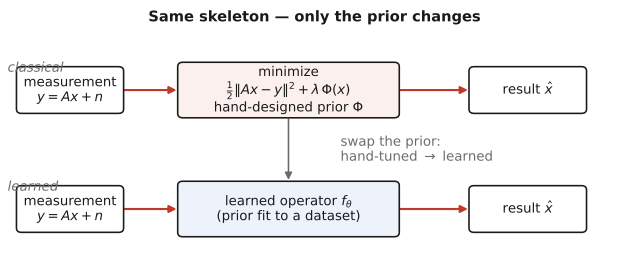
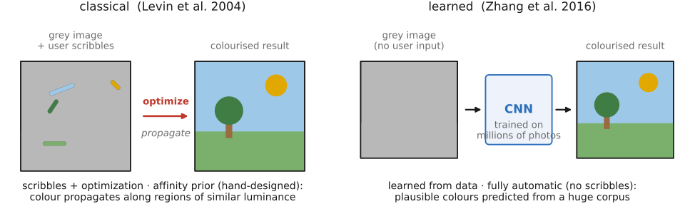
• **Learned filters — fit the penalty to data** — stop *hand-choosing* the basis/penalty and **learn** it: **Fields of Experts** (a Markov random field of learned filter responses, Roth & Black), **dictionary learning / K-SVD** (learn an overcomplete sparsifying dictionary), **trainable reaction–diffusion** (unroll a few diffusion steps and learn their filters). The prior is now **parametric and data-driven**, but still a stand-alone regularizer you plug into the same data-fit + prior solve.

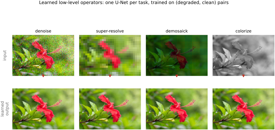
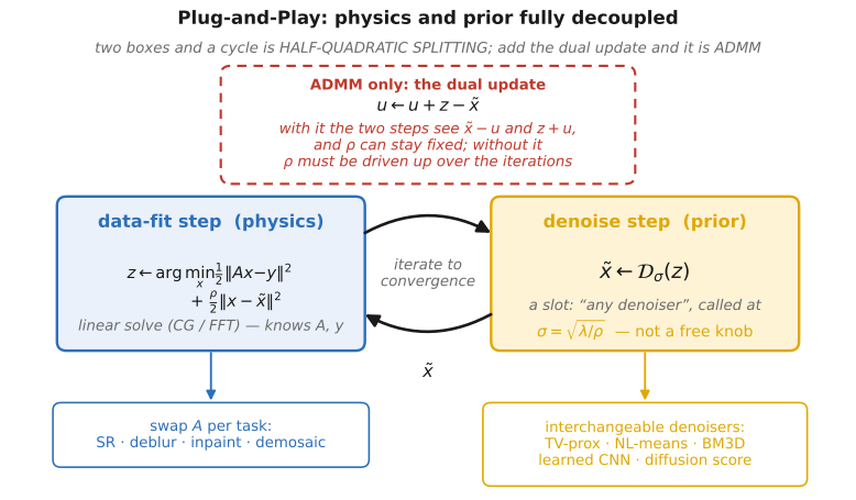
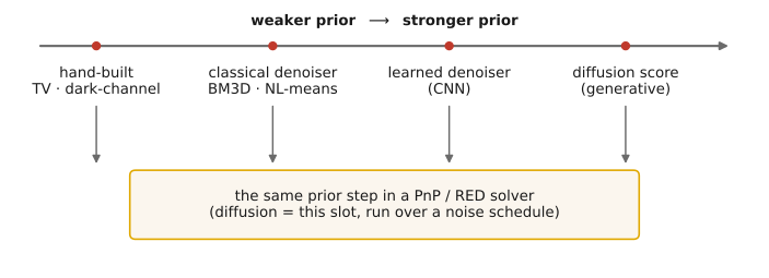
• **Denoising — the universal prior** — the limit of the previous rung: a *denoiser* already encodes "what natural images look like," so **any denoiser is a prior** (PnP / RED — next section). The catalog's hand-built penalties (Fourier, TV, wavelet, gradient) are just *explicit, weak denoisers*; classical (BM3D, NL-means) and learned (CNN) denoisers are stronger ones in the **same slot**.

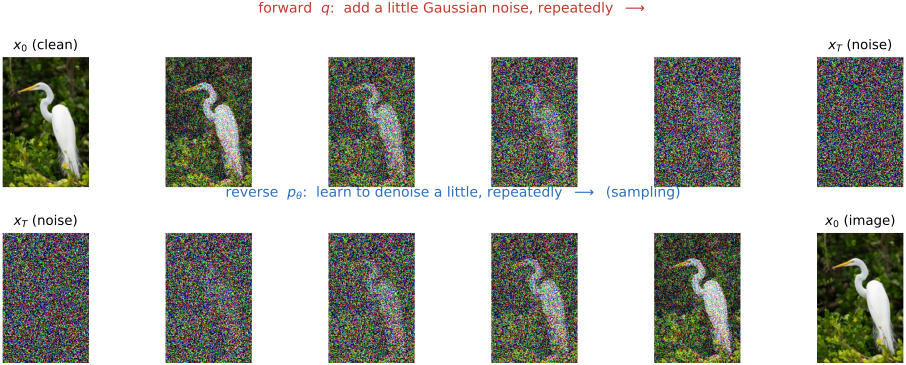
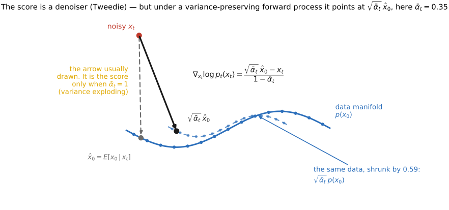
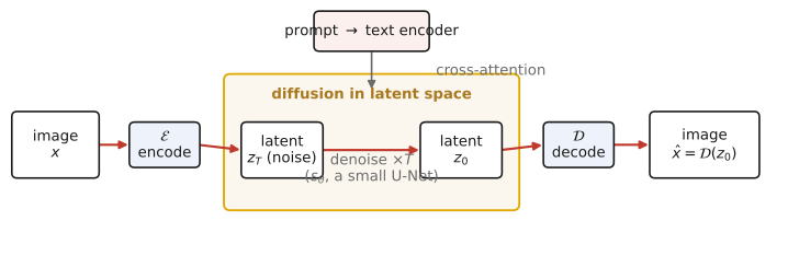
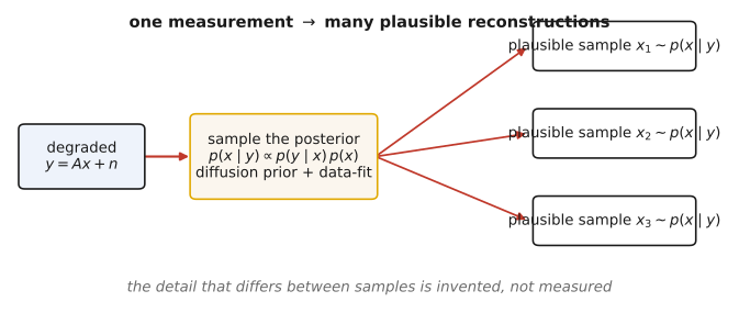
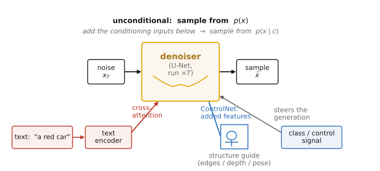
• **Diffusion — the strongest learned prior** — a denoiser trained over *all* noise levels, applied iteratively (next-but-one section): the most expressive point on the axis, the score of the natural-image distribution itself.

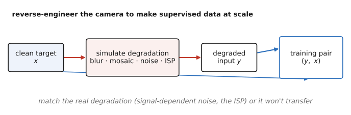
• **Joint learning — learn the inversion *and* the prior together** — the final move: stop treating the prior as a separable module. **Unroll** the iterative solver into a fixed number of steps and train the *whole reconstruction network* end-to-end on (measurement, ground-truth) pairs — **LISTA** (Gregor & LeCun), **ADMM-Net** (Yang et al.), **ISTA-Net** (Zhang & Ghanem), deep equilibrium / learned PnP. The "prior" is no longer something you can write down — it is **whatever weights make this forward operator's inversion best**, co-adapted to the physics $A$. (Cross-ref [[Deep learning]] — learned-operator lesson; and end-to-end optics+recovery in [[Computational optics and coded imaging#End-to-end optimization]].)

• 💡 **the arc**: fixed basis (Fourier) → fixed sparsity (wavelet/TV/gradient) → learned penalty (FoE/dictionary) → learned denoiser (PnP) → learned distribution (diffusion) → **prior + inversion learned jointly**. Each step trades **interpretability for expressiveness** (and needs more data). The next section shows the whole middle of this list is *one operation* — denoising.

• **Shift & scale invariance — the symmetries a prior should obey** — natural-image statistics are **translation-invariant** (stationary → the *sum-of-local-terms* form of the penalties above, Markov random fields, weight-shared CNNs) and **scale-invariant** (self-similar across zoom; signature = the **$1/f$ power spectrum** → multi-scale bases / pyramids / architectures). Less *extra* priors than the **shape every prior should have** — and the model that bakes both in by construction is dead leaves (next). [@field-1987; @ruderman-1997]

• a **special, oriented form of sparsity**: not just "few non-zero gradients" but "where it varies, it varies in **one direction**." Near an edge the image is locally a **1-D signal in 2-D** — its gradient field locally **rank-one**.

• **implicit in many algorithms, usually unnamed**: edge-aware filtering ("smooth *along* edges, not across") — anisotropic diffusion (Perona–Malik), bilateral; **demosaicking** — interpolate **along the local edge direction**, never across (edge-directed / homogeneity-directed), because color channels co-vary along the edge; joint demosaick-denoise; edge-aware upsampling.

• naming it as a prior explains the shared **failure mode**: fine **isotropic texture** (foliage, fabric) is *not* locally 1-D → the assumption is wrong → demosaicking **zippering** + color fringing.

• a prior on **how local colors are arranged**, not where the image varies: the pixels in a small window lie on a **short line / low-dim affine set** in RGB (a patch = 1–2 materials under smooth shading = a **linear mix** of a few endpoints — the **color-line model**).

• the elegant payoff — **Anat Levin's closed-form matting**: assume $F,B$ locally constant/linear ⇒ **$\alpha$ is a *linear* function of the local colors $I$** ⇒ eliminate $F,B$ analytically ⇒ a **quadratic in $\alpha$** = the **matting Laplacian**, one global **closed-form** linear solve. The hard nonlinear matting collapses to a linear system purely from a local linear color prior.

• recurs across the book: **dehazing** (haze-line / dark-channel), **demosaicking** (channels co-vary), denoising, white balance. Lesson: **a prior need not be about smoothness/sparsity** — a low-dim model of the local *color distribution* is just as much an image prior.

• **the unifying move**: in $\hat{x} = \arg\min_x \tfrac12\lVert Ax - y\rVert^2 + \lambda\Phi(x)$, splitting algorithms (**ADMM / HQS**) separate the two terms into alternating steps. The regularizer step turns out to be **exactly a denoising operation** (the proximal operator of $\Phi$ = "find the nearby image the prior likes" = denoise). [`fig-pnp-loop`]

• **Plug-and-Play (PnP) priors** (Venkatakrishnan 2013): so **drop in *any* denoiser** $\mathcal{D}_\sigma$ for that step — even one with **no closed-form prior** (BM3D, NL-means, a learned CNN). Alternate:

• **data-fit step**: $z \leftarrow \arg\min_x \tfrac12\lVert (k*x)\downarrow_s - y\rVert^2 + \tfrac{\rho}{2}\lVert x - \tilde{x}\rVert^2$ (enforce the measurement; a linear solve — CG/FFT, per [[Image formation as a linear system]]);

• **denoise step**: $\tilde{x} \leftarrow \mathcal{D}_\sigma(z)$ (impose the prior — *any* denoiser).

• payoff: **decouples** the imaging physics (the forward model $A$, swap per task — SR, deblur, inpaint, demosaic) from the **image prior** (the denoiser). One good denoiser ⇒ a solver for *every* inverse problem. (FlexISP, Heide 2014, builds a whole ISP this way.) [`fig-denoiser-as-prior-spectrum`]

• **RED (Regularization by Denoising)** (Romano 2017): make the prior **explicit** from a denoiser. Define $\Phi(x) = \tfrac12 x^\top(x - \mathcal{D}(x))$; under mild conditions its **gradient is just the denoising residual**, $\nabla\Phi(x) = x - \mathcal{D}(x)$. Then plain **gradient steps** minimize the regularized objective — the denoiser defines an actual energy, not only an opaque proximal step. (PnP ≈ proximal/implicit; RED ≈ explicit-gradient.)

• **why "universal"** (the section's headline): the **denoiser is the prior**. Improve the denoiser and *every* recovery task improves for free. This reframes "image prior" from a hand-derived penalty (TV, sparsity) to "whatever your best denoiser knows." [`fig-denoiser-as-prior-spectrum` — the spectrum from TV → BM3D → learned → diffusion]

• 💡 **callback to L5.4**: PnP/RED is the *mechanism* by which the not-optional prior enters — the denoise step IS the prior step.

• **Tweedie's formula**: for a Gaussian-noised observation $z = x + \sigma\epsilon$, the **MMSE denoiser** (posterior mean) is $\hat{x} = z + \sigma^2\,\nabla_z \log p_\sigma(z)$. So the **score** $\nabla_z \log p_\sigma(z)$ and a **Gaussian denoiser** are the *same object* (one is the other rearranged). [`fig-denoiser-as-prior-spectrum`, right end]

• **therefore diffusion = iterated denoising**: a diffusion model learns the score at every noise level; **sampling** repeatedly applies "denoise a little, add a little noise, repeat" from pure noise down to a clean image. That outer loop is precisely **PnP/RED taken to the continuous limit** — the prior-step denoiser is the learned score, run over a noise-level schedule.

• **consequence for recovery**: conditioning diffusion sampling on a measurement ($y$ via the forward model $A$) = a PnP/RED solver whose prior is the strongest learned denoiser we have → state-of-the-art SR / deblur / inpaint. This is the bridge from this chapter's *prior* story to generative models.

• **forward-ref**: the full diffusion treatment (DDPM, latent diffusion, score-matching, samplers) is in [[Generative AI and diffusion]]; here we only establish the **identity** denoiser ≡ score ≡ diffusion-step, closing the prior throughline. The diffusion chapter cross-refs back to *Denoising as a universal prior*.

• **closing idea** (hand-off to [[Blind deblurring]]): the same "data-fit + prior, and the prior is doing the heavy lifting" story now plays out where the **forward operator itself is unknown** — blind deblurring — and where hand-built priors (dark-channel) still earn their keep.

• **score-based models & the thin manifold**: the natural-image **manifold is thin** (≈ measure-zero) → the score $\nabla\log p$ is undefined/unreliable *off* it, exactly where a sampler lives. Fix (**Song & Ermon 2019**): **add Gaussian noise at many scales to *thicken* the manifold** so $p_\sigma$ has support everywhere and its score points back; train the score at every $\sigma$, sample by annealed Langevin (denoise-a-little / renoise-a-little). *This is why diffusion adds noise.* What the learned score captures about the manifold's **geometry** is active research (**Kadkhodaie, Guth, Simoncelli & Mallat 2024** — geometry-adaptive representations).

• **imperfect priors — don't plug neatly into Bayes**: a diffusion model lets you *sample/score* the prior but gives **no tractable likelihood / normalizer** — the prior is only **implicit** in the sampler. Conditioning on $y$ needs the posterior score $\nabla\log p(y\mid x)+\nabla\log p(x)$, whose data term is **intractable**, so every scheme (DPS/DDRM/ΠGDM) **approximates** it → measurement-consistency drift + hallucination. **Feng et al. 2023 (Bouman)** study when diffusion is a *principled* prior and what the approximations cost. Summary (per FUNDAMENTALS): astonishing priors, harder to stay faithful to the measurement — open research, not a plug-in.

• the goal of the section: give the **working vocabulary**, not a course. Keep it high level and intuitive; the imaging payoffs are the point.

• **entropy** $H(X)=-\sum p\log p$ — the average number of bits to name an outcome; the **fundamental limit of lossless compression** (Shannon's source-coding theorem). Low entropy = predictable = compressible.

• **mutual information** $I(X;Y)$ — how much knowing one variable tells you about another (shared information); the workhorse when *two* signals must be related (registration, channels).

• **relative entropy / KL divergence** $D_{\mathrm{KL}}(p\,\|\,q)$ — the coding cost of using the wrong distribution; *not* a distance (asymmetric), but the natural "how far is my model from the truth" term — and the thing hiding inside the VAE objective below.

• **channel capacity** $C=\max I(X;Y)$, and for an additive-Gaussian channel $C=\tfrac12\log_2(1+\mathrm{SNR})$ per use — the **maximum reliable rate** through a noisy pipe. The single formula the imaging-as-channel tradition runs on.

• **rate–distortion** $R(D)$ — the minimum bits to describe a source within an allowed distortion $D$ (**lossy** source coding). The literal optimization framework behind lossy compression; the curve every codec is trying to sit on.

• the honest framing for the rest of the chapter: **genuinely load-bearing in a few places, loosely invoked in many** — and naming which is which is the useful service this chapter does.

• **lossy image and video coding is not information-theory-*flavored*, it is information theory.** This is the one place the connection is exact, not analogical.

• **rate–distortion theory** (Shannon's lossy source coding) is the *literal* optimization framework: minimize bits subject to a distortion budget, the codec living on the $R(D)$ curve. [`fig-rate-distortion-jpeg`]

• **entropy coders** — Huffman, arithmetic, range coding — are **direct instantiations of the source-coding theorem** (reach the entropy bound for the symbol distribution you model).

• **transform coding** — the DCT (JPEG), wavelets (JPEG 2000) — is a **decorrelation strategy** for *approaching* the entropy bound: rotate into a basis where coefficients are nearly independent and energy-compacted, then quantize and entropy-code. **Every JPEG is a Shannon monument.**

• 💡 **the caveat an expert keeps front of mind**: the **distortion $D$** in $R(D)$ is almost always **MSE** (or something equally **perceptual-blind**). The entire history of **perceptual coding** is the engineering effort to **smuggle the human visual system back** into a formalism that does not natively want it — quantization matrices, CSF weighting, perceptual metrics. This MSE-vs-perception tension is the recurring theme of the whole chapter (it returns in §revival and §limits).

• the older, now somewhat **underappreciated** lineage: treat the **optical system as a band-limited noisy channel** and apply Shannon's capacity formula **across spatial frequencies**.

• the mid-century enthusiasm: **Fellgett & Linfoot** on the *assessment of optical images* (mid-1950s); later **Cox & Sheppard** casting **information capacity as a space–bandwidth–SNR product**. The capacity integral $$C=\int \log_2\!\big(1+\mathrm{SNR}(f)\big)\,df$$ sums $\log_2(1+\mathrm{SNR})$ over the spatial frequencies the system passes. [`fig-imaging-channel-capacity`]

• the deepest result in this vein — **Toraldo di Francia, "Resolving power and information" (1955)**: resolution is **not diffraction-limited in any absolute sense, it is information-limited**; **prior knowledge buys you super-resolution.** This aged extremely well and **quietly underwrites every modern prior-based reconstruction argument** (tie back to [[Fundamentals#Imaging as Bayesian inference with probabilistic priors]] — a prior is the extra information that re-opens what the operator closed).

• the **scientific-imaging branch is fully mature and standardized**: **DQE** (detective quantum efficiency) $=(\mathrm{SNR}_{\text{out}}/\mathrm{SNR}_{\text{in}})^2$ and **noise-equivalent quanta (NEQ)** are explicit **information-efficiency** measures — load-bearing in **x-ray, astronomy, and detector design** (**Rose's detectability criterion** sits adjacent). *If you are imaging photons for **measurement** rather than aesthetics, this machinery is real and used daily.* (→ [[Computational sensors]].)

• a cluster of **clean, specific** uses where an info-theoretic quantity is the actual objective function:

• **mutual information for multimodal registration** (Viola & Wells 1997; Maes et al. 1997) — about as direct as it gets: **CT/MRI alignment** maximizes $I$ between the two modalities' intensities. Genuinely load-bearing.

• **maximum-entropy deconvolution** (Gull & Skilling; Frieden) — enormously influential in **radio interferometry and spectroscopy**; *but* largely **absorbed into the broader Bayesian / sparsity prior-design** conversation, where the entropy term reads as **one convenient regularizer among many** rather than uniquely principled. (Honest: this one has faded into the general prior toolbox.)

• the **multiplex / Fellgett advantage** behind **coded apertures and Hadamard multiplexing** is **SNR-and-information** reasoning (measure sums of many sources at once, win SNR; → [[Computational optics and coded imaging]]).

• **plenoptic sampling** (Chai et al. 2000) is a **degrees-of-freedom** analysis of the light field — how densely you must sample rays (→ [[Light fields and plenoptic cameras]]).

• worth flagging because it is **not nostalgic**: information theory came *back*, through compression and density modeling.

• **learned image compression** (Ballé et al. and successors) is **end-to-end rate–distortion optimization with neural entropy models** — the **"entropy bottleneck"** and **hyperprior** are **Shannon and deep learning fused without apology**, arguably the cleanest contemporary instance.

• the **generative stack carries information theory in its bones**: the **VAE ELBO** is *reconstruction minus a relative-entropy (KL) term*; **β-VAE** is an explicit **rate–distortion knob**; **MDL** and **bits-back coding** give the **likelihood-as-codelength** reading; **diffusion's variational bounds** inherit the same structure. (→ [[Generative AI and diffusion]].)

• the arc to state: the field that **nearly walked away** from information theory mid-century **walked right back into it** through compression and density modeling.

• several things commonly lumped in are **cousins, not children**; being precise here is a service:

• the **Nyquist–Shannon sampling theorem** bears Shannon's name and shares the degrees-of-freedom intuition, **but it is a statement about band-limited reconstruction, not about information content** — conflating the two is a frequent sloppiness (keep separate from the sampling-theorem treatment in [[Basic image processing and ISP#Sampling, downsampling, and aliasing]]).

• **compressed sensing** is **sparse linear recovery** (RIP, $\ell_1$), with an information-theoretic *flavor* in its **sample-complexity bounds** but **not a Shannon construction at heart** (→ [[Computational optics and coded imaging#Compressive sensing]]).

• **"image entropy"** as an **autofocus / sharpness metric** is a **single-symbol histogram quantity** — useful, but a **thin shadow** of the real theory.

• the candid bottom line: information theory has been **genuinely less relevant to exactly the half of the field that makes photography *photography*** rather than imaging — **aesthetics, tone, color, perceptual quality**.

• **entropy does not know that a slightly noisier but sharper image looks better**, and the formalism has **nothing to say about what makes a photograph *good*.**

• the **perception–distortion tradeoff** (Blau & Michaeli 2018) is almost a **confession** of this: a quasi-information-theoretic proof that **fidelity and perceptual realism are in tension** — the clean $R(D)$ story and human judgment **pull apart**. [`fig-perception-distortion`]

• 💡 **placement on the measurement-to-synthesis spectrum**: information theory is **overwhelmingly a measurement-and-transport-side tool** — strongest describing how efficiently a system **captures, stores, and moves** image data, and **weakest the moment the target quantity becomes perceptual or aesthetic**, which it was never built to represent. (This is the same measurement-vs-perception seam that opened in §compression and runs through the whole chapter.)