Lecture Notes 7 — HDR 2, bilateral grid⧉
Course notes cut from Computational Photography, an AI-powered Slopendium for this lecture. Each section links back to its home in the book; sections marked optional go beyond what the lecture needs.
Contents · 19 sections on this page, from 10 chapters of the book
Titles jump to the section below; ↗ opens it in the book.
Adaptation and constancy⧉
Visual perception is largely invariant to multiplications⧉
optionalA cloud can reduce the light on a page while leaving its print recognizably black on white. Ratios between surface luminances can remain unchanged even though the overall scene looks dimmer. This approximate stability concerns surface appearance and discrimination; it does not mean the observer cannot detect a change in illumination.
The mechanism is gain control, and gain control is multiplication. A photoreceptor in a bright field turns its sensitivity down, one in dim light turns it up, and each does so, to a first approximation, by scaling its response by a factor set by the local average. Chromatic adaptation is the same operation run channel by channel: the von Kries model is an independent multiplicative gain on each cone class, the diagonal model we use for white balance. Light adaptation, from the previous section, is its achromatic version.
In a simple matte-surface model, luminance is proportional to illumination times reflectance. Ratios between nearby surfaces cancel a shared illumination factor. Shadows, interreflections, specular reflection, and different surface orientations can violate that shared-factor assumption. Local gain control helps explain some stability, while spatial organization and interpretation supply other cues.
Changing exposure time or aperture scales the expected sensor signal within the linear, unclipped regime. ISO changes gain and camera behavior; it does not itself increase the photons captured. Exposure is measured in stops because a stop corresponds to a factor of two. These multiplicative descriptions are useful for processing, but changing exposure does not reproduce visual adaptation.
The experimental record is old and specific. Wallach showed that the perceived lightness of a disk is fixed by the ratio of its luminance to its surround: hold that ratio and the gray looks the same through a hundredfold change in absolute light Wallach 1948 (ratio principle). Land and McCann built Retinex on the same principle, computing lightness from ratios taken along spatial paths so that slow illumination gradients fall away Land & McCann 1971. Gilchrist's Seeing Black and White gathers decades of such findings into an account of how vision anchors lightness and assigns it across a scene Gilchrist 2006 (Seeing Black and White).
The stability is partial and task-dependent. Surface-lightness matches can remain relatively constant where brightness matches change Arend & Goldstein 1987. Constancy also depends on available scene cues Kraft & Brainard 1999. At low light levels, photon and neural noise, receptor changes, and threshold behavior limit a simple gain model.
A ratio can be invariant to a common scale without any logarithm. For positive $I$ and a positive local estimate $B$, scaling both by $\alpha>0$ leaves $I/B$ unchanged. A logarithm represents the same ratio as a difference:
The offset introduced by scaling cancels in the difference. The individual log values change, so log encoding is not itself invariant. Divisive normalization and logarithmic coordinates are related mathematical tools, not interchangeable claims about neural implementation.
A stored HDR image can use linear floating point, log encoding, or another transfer function. Log values make exposure changes additive and provide approximately relative precision over positive values. They are useful, not mandatory. Encoding choice must also handle zero, negative intermediates, quantization, and the operations to be performed (Chapter 4.3, Encoding: linear, gamma or log).
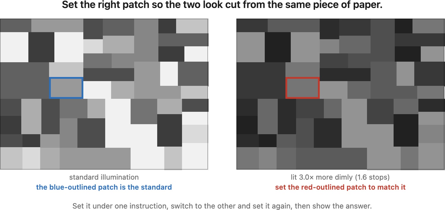
Shared multiplicative changes preserve ratios and often leave surface appearance approximately stable. Brightness, visibility, and color can still change. Gain-control models are useful within their assumptions; they do not make vision insensitive to illumination.
Dividing a value by a similarly scaled reference cancels a common multiplier. Taking logarithms turns the ratio into a difference. This explains why log coordinates are useful for relative changes, without claiming that vision uses a global logarithm or that HDR storage requires one.
Consider two matte patches side by side under the same illumination. In a scalar illumination–reflectance model, doubling the illumination doubles both luminances, but leaves their ratio unchanged. That ratio therefore carries information about the relative surface reflectances without requiring the observer to know the illumination level. Put one patch into a cast shadow and the cancellation no longer holds: the two patches now have different illumination factors. The visual system needs spatial context to decide whether a change is a material boundary or a lighting boundary. This is the connection between multiplicative image formation, ratio-based descriptions of contrast, and the harder inference problem of constancy.
Spatial and temporal vision⧉
Spatial vision⧉
optionalHow fine a pattern can we resolve, and how does sensitivity vary with the scale of the detail? Visual acuity (the familiar eye-chart measure) sets the finest line spacing we can make out, but it is only the high-frequency tail of a larger story.
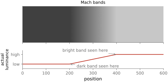
Many retinal neurons have center–surround receptive fields, comparing signals over neighboring regions. Such models can produce edge overshoots resembling Mach bands Mach 1865 (Mach bands) (Figure 3.4.1). They illustrate one contribution to spatial processing; no single lateral-inhibition filter explains every lightness illusion.
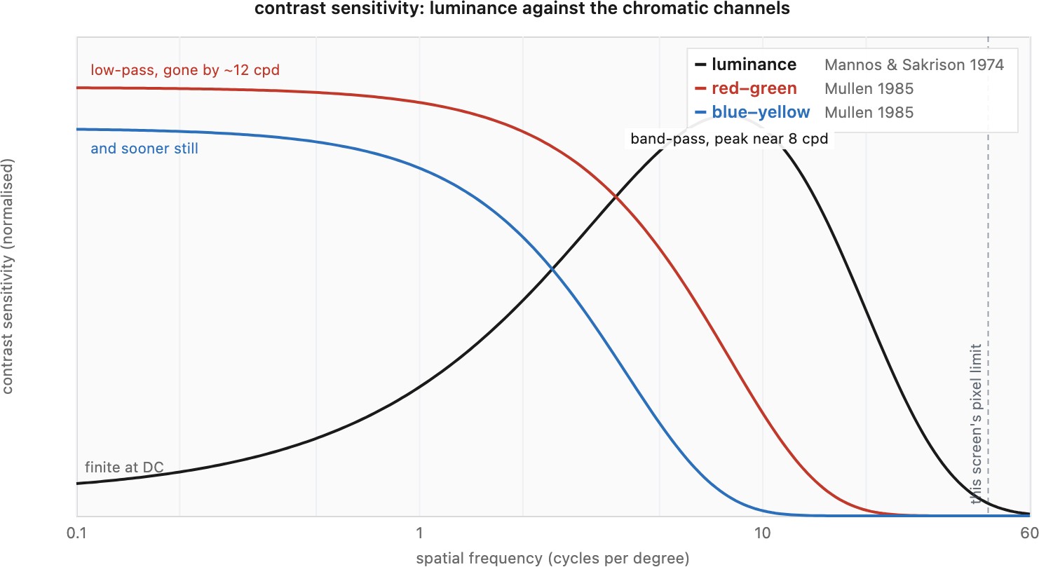
A contrast sensitivity function (CSF) describes detection thresholds for specified stimuli, often sinusoidal gratings. Sensitivity is the reciprocal of threshold contrast. Under common photopic conditions, luminance sensitivity is band-pass: intermediate spatial frequencies are easier to detect than very coarse or very fine gratings. The curve changes with viewing conditions.
This experiment can be reproduced directly (Figure 3.4.2). In the Campbell–Robson chart Campbell & Robson 1968, spatial frequency rises to the right and contrast rises downward, the same contrast range in every column, yet the height at which the stripes fade into flat gray is an inverted U, not a level line. The visibility boundary traces the observer's contrast sensitivity function. And because the CSF is measured in cycles per degree of visual angle, the boundary moves with viewing distance: step back and the fine bars on the right vanish first.
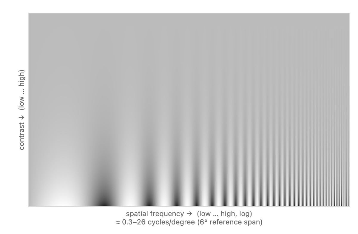
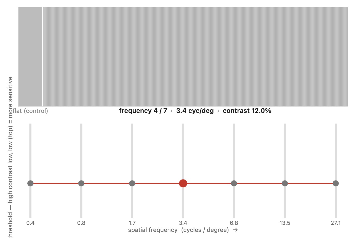
Figure 3.4.3 lets you adjust grating contrasts at several spatial frequencies. It illustrates a method-of-adjustment experiment. The display transfer function, ambient reflections, pixel sampling, and quantization affect the result; sRGB encoding and dithering alone do not calibrate an arbitrary screen.
The Mannos–Sakrison fit provides a compact relative frequency weighting Mannos & Sakrison 1974:
Here $f$ is spatial frequency in cycles per degree. The curve peaks near 8 cycles/degree. It has no hard high-frequency cutoff and is not, by itself, a calibrated absolute detection threshold for the reader. Its value at zero frequency should not be interpreted as a universal ability to detect a uniform field change. Evaluated, it gives relative weights of about 0.32 at 1 cycle/degree, 0.98 near the 8 cycle/degree peak, 0.19 at 30 and 0.004 at 60: an error pattern at 30 cycles/degree counts about a fifth as much as the same pattern near the peak, and one at 60 barely counts at all.
Convert image frequency to angular frequency before using such a model. For a centered display of width $w$ viewed at distance $d$, the horizontal angular span is
A pattern with $m$ cycles across that width has average frequency $f=m/\theta$. For example, 30 cycles across 10 degrees gives 3 cycles/degree. This average is a useful small-field approximation; a wide perspective display needs the local pixel-to-angle mapping.
A more complete luminance model also accounts for the light level and the size of the test. Barten's work Barten 1999 is an important example, with applications to display encoding. The compact Mannos–Sakrison curve is useful when a relative weighting by spatial frequency is enough; it should not silently replace the richer conditions of an absolute visibility prediction. This is the engineering purpose of a CSF: errors at different angular frequencies need not receive the same weight.
The eye is not equally sensitive to every spatial frequency. Luminance sensitivity is band-pass, peaking at a few cycles per degree and falling away on both sides, and the curve moves with light level, field size and contrast. It is defined per degree of visual angle, not per pixel, so viewing distance and display size decide which frequencies a reader can resolve at all. Quote a peak from a textbook and you have described one experiment's conditions; measure it in the conditions you ship in.
File formats and compression⧉
JPEG: compression by perception⧉
optionalThe common baseline JPEG path Wallace 1991 combines lossy quantization with lossless entropy coding. Color conversion and optional subsampling commonly precede the block codec. JPEG also specifies modes beyond this baseline; the following description concerns the usual 8-bit photographic workflow.
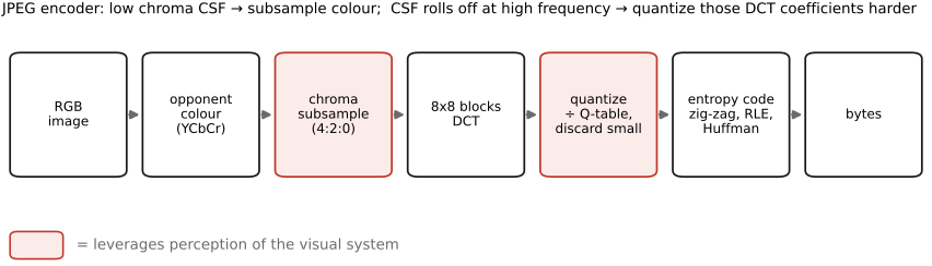
Y from two chroma channels Cb, Cr. (2) Chroma subsampling: shrink Cb and Cr to half resolution (4:2:0), exploiting the eye's low color acuity. (3) Block DCT: split each channel into 8×8 blocks and transform each to spatial-frequency coefficients. (4) Quantization: divide the coefficients by a quality-dependent table that crushes high frequencies hardest; this is the only lossy step. (5) Entropy coding: losslessly pack the (mostly zero) quantized coefficients in a smart order. Decoding runs the same chain in reverse.The starting observation, lifted straight from Chapter 3.4, Spatial and temporal vision, is that human vision is not uniform. The contrast sensitivity function (CSF) tells us our sensitivity to detail falls off at high spatial frequencies: we simply cannot resolve fine texture as well as coarse structure. And our sensitivity to color detail is far lower still than our sensitivity to brightness detail: the eye has sharp acuity for luminance and surprisingly coarse acuity for hue. JPEG's entire strategy is to match the number of bits to what the eye can actually use: many bits for the brightness structure we see keenly, few for the color detail and the high frequencies we barely register. The five stages below implement that allocation.
Bilateral filtering⧉
PS2 implements the bilateral filter (with a YUV chroma variant). → Chapter 1.5, Problem sets (appendix).
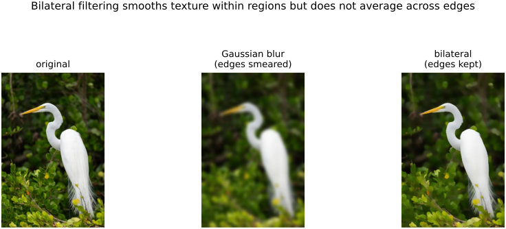
A blur mixes two sides of an edge and makes it soft. That is useful for some operations, but harmful when we want to remove noise while preserving sharpness or to smooth texture while keeping the boundary. The big idea of the bilateral filter is to only take into account pixels that are similar enough. This notion of affinity between pixels will come back over and over for edge-preserving techniques.
We illustrate bilateral filtering for the task of denoising, but it also underlies many algorithms because it enables the factoring of images into large-scale structure and local detail while preserving strong edges. This proves powerful for applications such as high-dynamic-range tone mapping (Chapter 18.3, Two-scale and bilateral tone mapping), upsampling low-resolution results, and combining images with different illumination, where the edges come from a second image (#Cross / joint bilateral).
Debugging: hand-checkable limits⧉
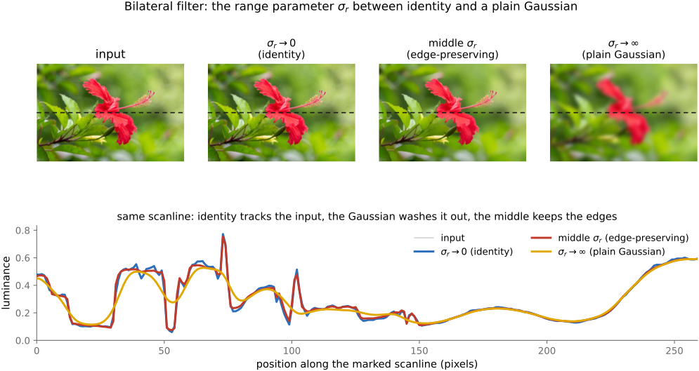
The bilateral has two limits you can predict by hand, and together they make an excellent correctness test for an implementation (Figure 10.1.7). Push the range width to each extreme:
- Large range variance ($\sigma_r \to \infty$): the range Gaussian flattens, $g_r \to 1$, so it does nothing: every value difference counts as "similar." The weight reduces to the spatial Gaussian alone, and the bilateral collapses to a plain Gaussian blur.
- Tiny range variance ($\sigma_r \to 0$): only neighbors with the same value retain weight in the limit. They may include many pixels, but averaging equal values leaves the output unchanged. Averaging those equal values changes nothing, and the output is the identity: the image comes back untouched, edges and all.
A middle $\sigma_r$ interpolates between these two: enough to smooth away noise and texture, not so much that it bleeds across real edges. If your implementation does not reproduce a Gaussian at large $\sigma_r$ and the identity at small $\sigma_r$, it is wrong. These are the first two things to check (and the recipe in the debugging sidebar above).
The same two knobs guide tuning. Pick $\sigma_s$ from the spatial scale of the structure you mean to remove (how large a region should be pooled). Pick $\sigma_r$ from the contrast of the edges you mean to preserve: set it just below the value jump of a real edge, so the filter smooths everything gentler than that and stops at anything sharper. And state the encoding first: the same numeric $\sigma_r$ means something completely different in linear light, in gamma, and in log luminance.
Bilateral filter⧉
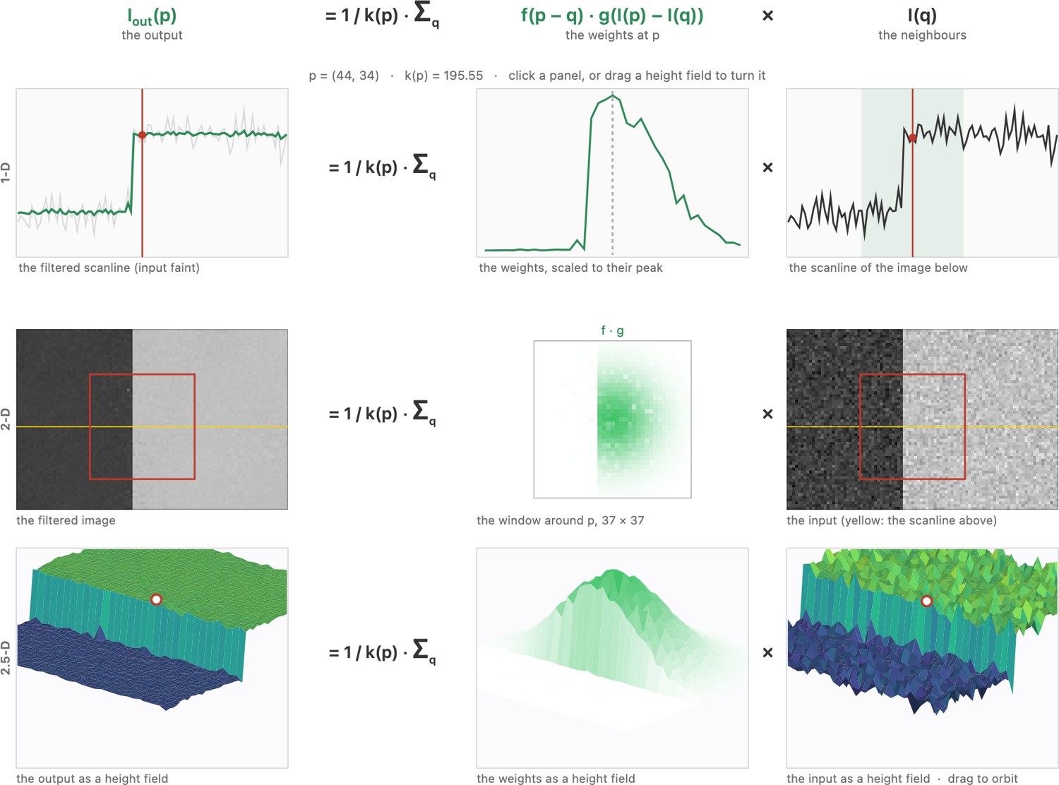
optionalConsider an input signal composed of a step edge with noise (Figure 10.1.1). The goal of bilateral filtering is to remove the noise by averaging nearby pixels without blurring the edge.
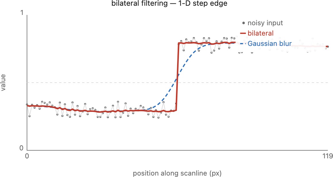
Start from the Gaussian blur. It replaces each pixel with a weighted average of its neighbors, where the weight only depends on distance. It is a spatial Gaussian $g_s(\lVert p - q\rVert)$ of the distance between the center pixel $p$ and a neighbor $q$: nearby pixels count for a lot, distant ones taper off. It is easiest to watch this on a 1-D scanline (a single row of the image), where the picture becomes a wiggly curve of value against position (Figure 10.1.1).
The trouble, once more, is the edge. A step edge on the scanline, with values low on the left and high on the right, gets smeared by the Gaussian, because right at the step the averaging window reaches across the boundary and blends the two plateaus together. The same bleed, in two dimensions and on a compressed base layer, is what paints halos along high-contrast edges in tone mapping (Chapter 18.3, Two-scale and bilateral tone mapping).
The fix is a single extra factor. Keep the spatial Gaussian, but multiply in a second Gaussian, this one on the value difference between the center pixel and the neighbor, $g_r(\lvert I_p - I_q\rvert)$. This range weight asks "are these two pixels similar in value?" and down-weights neighbors that are too different. A neighbor that is close in space but far in value, one on the other side of an edge, now earns a weight near zero, however spatially near it sits. The filter, all by itself, declines to average across the edge.
A practical wrinkle follows. The range weight asks whether two pixels are similar. But on a badly corrupted image the raw values are an unreliable judge: noise can make two same-region pixels look different, or two different ones look alike, so the weights themselves come out noisy. The weights need not be read from the original image at all. We can compute $g_r$ from a pre-cleaned version (a quick median filter, say, or any cheap denoise) and then apply those steadier weights when averaging the original pixels. Decoupling what decides the affinity from what actually gets averaged is exactly the move the cross / joint bilateral (below) makes with a separate guide image; using a median-filtered copy of the same image as that guide is just the in-place version of the trick.
Putting the two Gaussians together gives the bilateral filter (Tomasi & Manduchi 1998). The weight a neighbor $q$ receives at pixel $p$ is the product of the spatial and range terms,
and the output is the normalized weighted average of the neighbors,
In words: "average my neighbors, but only those that are both nearby and similar to me." The two widths do different jobs. $\sigma_s$, in pixels, sets how large a region we pool over, the reach of the spatial Gaussian. $\sigma_r$, in intensity units, sets what counts as "too different": the value gap beyond which a neighbor stops counting. Because $\sigma_r$ is measured in the same units as $I$, we must fix the encoding before we can quote it: for HDR tone mapping the filter runs on log luminance (Durand & Dorsey 2002, where a range $\sigma_r \approx 0.4$ in $\log_{10}$ is typical); other tasks may use linear values or a specified output encoding. There is no single required domain for every bilateral application.
As code, the brute-force bilateral is a double loop with a per-pixel normalization, and one subtlety distinguishes it from convolution: you may precompute the spatial weight $g_s$ (it is the same window everywhere), but the range weight $g_r$ must be recomputed for every pair, because it depends on the value difference at that pixel. The range function can be tabulated for quantized differences; it is the resulting image-dependent kernel that cannot be reused as one convolution. Specify spatial truncation and boundary handling, include the center sample, and accumulate in a sufficiently wide type.
precompute g_s over the window          # spatial weights, same for every pixel
for each output pixel p:
    sum ← 0;  W ← 0                      # accumulator and normalizer
    for each neighbour q in the window around p:
        w ← g_s(‖p − q‖) · g_r(|I[p] − I[q]|)   # range term recomputed per pair
        sum ← sum + w · I[q]
        W   ← W + w
    I_bf[p] ← sum / W                    # per-pixel normalization
For a color image the range distance $|I_p - I_q|$ is the 3-D distance in RGB (or YUV); everything else is unchanged.
The filter also travels under other names in editing software. Photoshop's Surface Blur is a bilateral filter: its radius is the spatial width and its threshold is the range width, over a box spatial kernel rather than a Gaussian. The name is worth knowing: those two sliders are the two widths of this section, and a tool many readers already use is a direct way to feel what each one does.
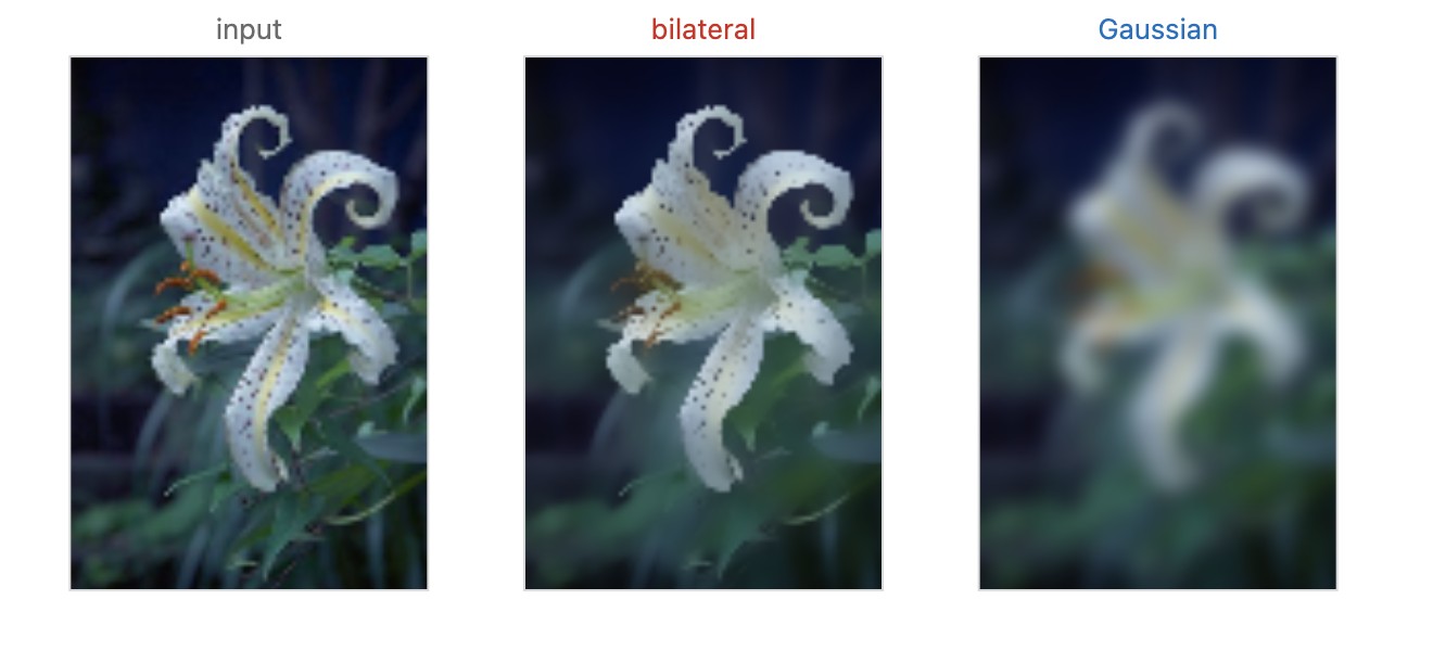
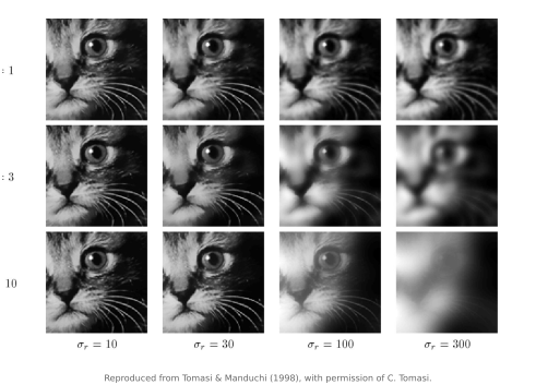
Two extreme settings of the range width $\sigma_r$ give two predictable outcomes that bracket the whole filter, the fastest way to sanity-check an implementation (the recipe also lives in Developing, testing & debugging). Figure 10.1.7
- Crank $\sigma_r$ very large. The range term flattens, $g_r \to 1$, and drops out of the product. The bilateral must collapse to a plain Gaussian, so run it side by side with your already-tested Gaussian blur; they should agree pixel for pixel.
- Shrink $\sigma_r$ very small. Now a pixel averages only with near-identical neighbors, so edges stay untouched and the output is essentially the input. Run it on a synthetic half-plane or rectangle (one hard edge): the bilateral must leave that edge razor-sharp.
If either limit misbehaves, the bug is in the range term or the normalization; fix that before trusting any middle $\sigma_r$.
The 1-D picture carries straight to the 2-D image: the bilateral smooths flat texture and noise inside each region while holding the edges, so a portrait emerges with clean skin and intact eyelashes, and an HDR base layer stops cleanly at the silhouette instead of ramping across it (Figure 10.1.2).
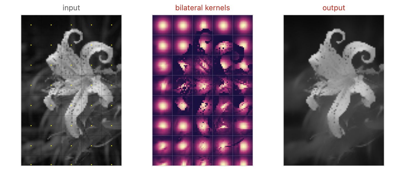
The range Gaussian $g_r$ is more than a clever weight; it is a similarity, an affinity between two pixels: a number that says how much these two pixels belong together, computed from their value difference. The bilateral averages pixels in proportion to that affinity. Every later method in this chapter, and several beyond it, is a different answer to one question: how should we measure whether two pixels belong together?
Use the color / intensity difference between two pixels as how much they belong together, an affinity, then average (or connect) pixels in proportion to it. Pixels with high affinity are treated as measurements of the same underlying thing and get averaged together; pixels with low affinity, across an edge, are kept apart. The bilateral filter's range weight $g_r$ is the first full instance, but the same affinity drives the bilateral grid, the guided filter, non-local means (NL-means), colorization, and matting / segmentation that follow. Edge-preserving is affinity. (This is L10.1, registered in Part 13, Denoising where the bilateral first appeared for noise; this is its full edge-preserving treatment.)
Robustness⧉
optionalWith the Gaussians defined above and the center included, $w(p,p)=1$, so $W_p\geq1$. The normalized bilateral is a convex average and cannot blow up from division by a near-zero normalizer. An isolated value can still be poorly denoised because it assigns little weight to other samples. This is a limitation of the affinity, not proof that normalization is numerically invalid.
The deeper weakness is that the range term reads the noisy image itself. At an outlier the center's own corrupted value decides which neighbors count as similar, so the pixel that most needs help is the one whose weights are least trustworthy: it finds nothing that resembles it and averages with almost nothing but itself. A hot pixel survives the filter for the same reason an edge does.
A cheap repair is to compute the range term from a pre-filtered copy instead of from the input. Run a small median filter first, then use that image as the reference for the value differences while still averaging the original samples. The median removes impulses without moving an edge (Chapter 13.3, Gaussian, median, and bilateral filtering), so the weights are decided by something close to the clean signal while the output remains an average of real measurements. Mechanically this is the cross-bilateral construction of the next section, with the guide derived from the input rather than captured separately.
The cost is that the guide's failures become the filter's. A median erases thin lines, small dots and isolated highlights, and a structure the guide has removed has no range weight left to defend it: the bilateral will happily average it away. Check the guide on the structures you care about before trusting the result, and keep the median's window small enough that it removes impulses rather than detail.
An alternative discussed by Aubry et al. is an unnormalized correction Aubry et al. 2014. Its scale must be defined. With these unnormalized spatial weights, introduce a step size $\eta$:
Each neighbor contributes a weighted difference from the center. A sufficient condition for this update to remain a convex combination is $0\leq\eta\sum_{q\ne p}w(p,q)\leq1$. One practical convention normalizes the spatial kernel to sum to one and uses $0\leq\eta\leq1$. Without a scale convention, adding more neighbors can cause overshoot. The update generally differs from the normalized bilateral; neither is a universal replacement for the other.
This unnormalized form is also the bilateral cousin of the local Laplacian filters: working in deltas from the input, scale by scale, is exactly the move that makes the multiscale local Laplacian fast and robust (Paris / Aubry; cross-ref Chapter 10.4, Local Laplacian filters and Chapter 6.6, Pyramids and wavelets).
Removing the bilateral normalizer changes the filter. Specify a normalized spatial kernel or an explicit step size, then test constants, impulses and edges. A small total affinity makes a small correction; it does not establish that an isolated value is correct.
Cross / joint bilateral⧉
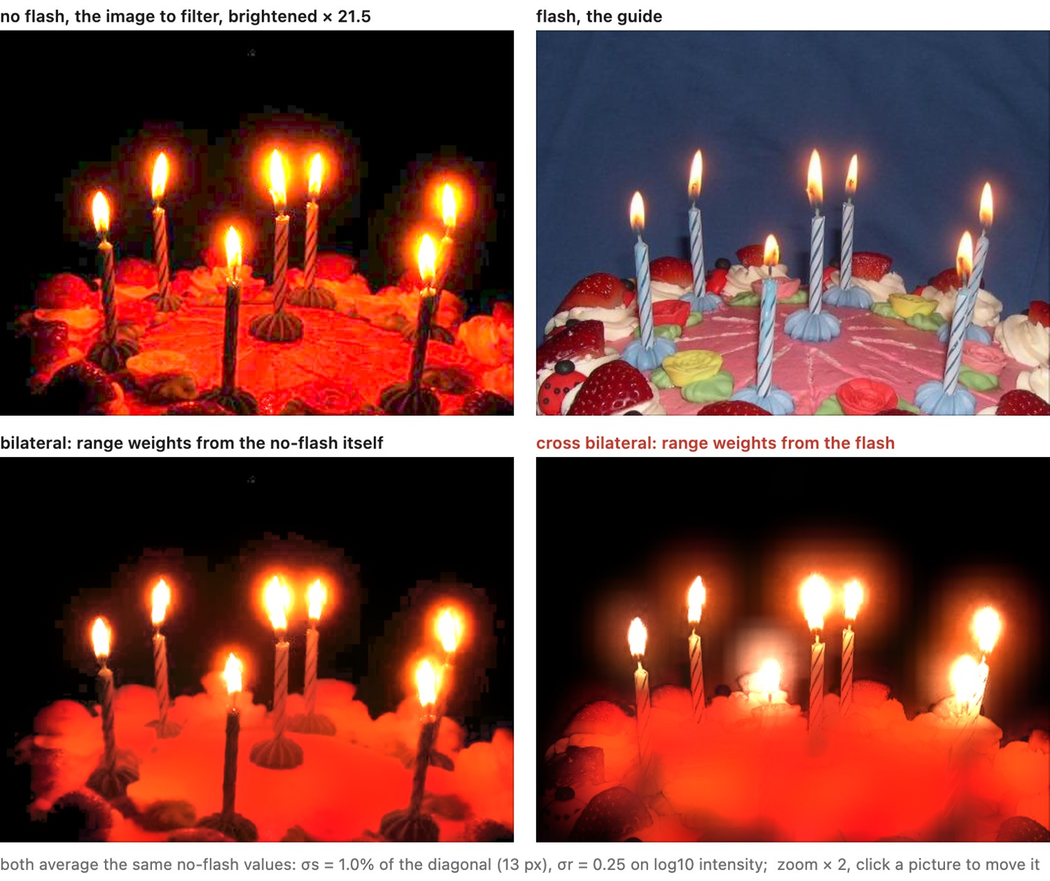
optionalSo far the affinity has been read off the same image we are smoothing (the range weight uses $I$ itself). But there is no reason it must. The cross (or joint) bilateral filter reads the range weight from a different image, a guide $J$, while still averaging the target $I$:
The averaging runs over the target $I$; the affinity comes from the guide $J$. Why want that? Because sometimes the image you wish to smooth is too noisy or too dark for its own edges to be trusted. If you read the affinity off $I$, you are reading off the noise. If you hold a cleaner signal that shares the same scene geometry, borrow its edges instead.
The headline application is flash / no-flash photography (Petschnigg et al. 2004; Eisemann & Durand 2004). Shoot a dim scene twice: once without flash (the right mood and color, but dark and noisy) and once with flash (clean and well-exposed, but flat, harsh lighting). After registration, many object boundaries correspond. Motion, occlusion, flash shadows and specularities can introduce mismatched edges, so a practical pipeline needs confidence masks or fallback behavior. So smooth the noisy no-flash image using the flash image as the guide: the flash image's clean edges drive the range weight, telling the filter where it may and may not average, while the values being averaged come from the ambient no-flash shot. The result keeps the no-flash mood and kills the no-flash noise (Figure 10.1.8). We develop the full flash/no-flash pipeline later (forward-ref → Flash / no flash, computational illumination).
The full flash/no-flash story, including Petschnigg's detail transfer, Eisemann & Durand's intrinsic-relighting pipeline, flash-shadow removal, and their end-to-end results, belongs with the rest of computational illumination, where capturing the scene under two lights is the whole subject (Flash / no flash).
The cross bilateral is the first instance of a more general joint / guided idea (filter one image using structure taken from another) that culminates in the guided filter (later in the part).
Bilateral grid⧉
The bilateral filter is non-linear: the weights depend on the pixel values, so they differ at every output pixel, and the whole thing is not a convolution. That is why you cannot reuse your fast Gaussian-blur code, and why a brute-force bilateral is a slow double loop. The bilateral grid (Chen, Paris & Durand 2007) is the observation that you can turn it back into an ordinary convolution: add a dimension (Figure 10.1.9).
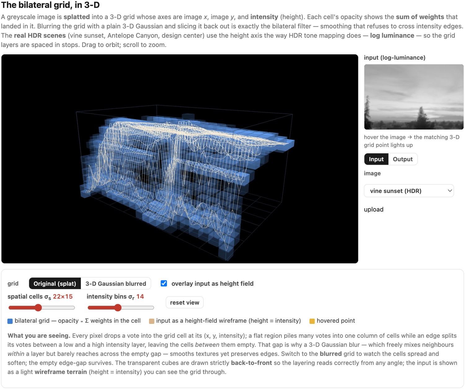
The key picture: the product of a spatial Gaussian (in $x, y$) and a range Gaussian (in $I$) is just a single 3-D Gaussian in the space $(x, y, I)$. So lift every pixel out of the 2-D plane into a 3-D space by using its value as a third coordinate. Pixel $(x, y)$ with value $I(x, y)$ goes to grid position $(x, y, I(x,y))$. In this lifted space the nonlinear 2-D bilateral becomes a plain, separable 3-D Gaussian blur, that is, an ordinary linear convolution, and the edge-preserving behavior is automatic: two pixels on opposite sides of an edge have very different values, so they land in different layers of the grid, which reduces their interaction according to the range bandwidth. A Gaussian still has nonzero tails, and discretization adds approximation error.
The bilateral is awkward because it is non-linear: its weights depend on the pixel values, so they differ at every output pixel and the filter is not a convolution. The bilateral grid's deeper trick, beyond "add a dimension", is to discretize the intensity (range) axis into a small set of levels, and then do cheap, ordinary linear work at each level. Quantize $I$ into grid layers, run a plain blur within and across layers (distant layers interact less, with accuracy controlled by grid resolution and the blur), and interpolate back to each pixel's exact value. The per-pixel nonlinearity becomes "a few linear passes plus a lookup." This is a general recipe, not a bilateral-only hack: the fast local Laplacian filter (Chapter 10.4, Local Laplacian filters, Aubry et al. 2014) accelerates its per-pixel nonlinearity the same way: evaluate a handful of discrete intensity levels of a slow operator and interpolate between them. Whenever a filter's cost comes from a continuous, value-dependent response, discretizing that response axis turns it into reusable, parallel, convolution-shaped work. (Registered in Big Lessons as L10.2; recurs in Chapter 10.4, Local Laplacian filters and, as an algorithm-level speedup, in Chapter 29.1, Algorithmic speedups.)
The pipeline has three steps (splat, blur, slice):
- Splat. Build a coarse 3-D grid indexed by $(x, y, I)$. For each pixel, accumulate two things into its cell: its value and a weight (a count of how many pixels landed there). Many cells receive no pixels and stay empty; the per-cell weight is exactly the bookkeeping that will reproduce the bilateral's normalizer.
- Blur. Convolve the grid with a plain separable 3-D Gaussian, an ordinary blur along each axis in turn (the $[1\ 4\ 6\ 4\ 1]/16$ stencil if the Gaussian is one cell wide). Blur both the accumulated values and the weights. Spatial smoothing and range smoothing both fall out of this single convolution; mixing across layers is attenuated according to the range kernel.
- Slice. Read the result back out at each pixel's own location $(x, y, I(x,y))$ by trilinear interpolation, and divide the interpolated value by the interpolated weight: that division is the bilateral normalizer $1/W_p$, recovered for free.
The whole pipeline is short, and every step is an ordinary operation (accumulate, blur, look up):
# splat — build the coarse grid (downsample by σ_s in space, σ_r in range)
for each pixel (x, y):
    c ← (x/σ_s, y/σ_s, I[x,y]/σ_r)      # the cell this pixel lands in
    splat(grid, c, I[x,y])              # distribute to surrounding vertices
    splat(weight, c, 1)                 # same interpolation weights

# blur — plain separable 3-D Gaussian, on BOTH grid and weight
blur grid, weight along x, then y, then I    # e.g. [1 4 6 4 1]/16 per axis

# slice — read back at each pixel's own (x, y, I), normalized
for each pixel (x, y):
    c ← (x/σ_s, y/σ_s, I[x,y]/σ_r)
    out[x, y] ← interpolate(grid, c) / interpolate(weight, c)      # trilinear interpolation at c
return out
Why is this fast? Because the grid is coarse. The right resolution is set by the filter's own widths (a grid cell about $\sigma_s$ wide in space and $\sigma_r$ deep in range), so the grid is heavily downsampled in both space and value, often by large factors. A small grid, a separable blur, a trilinear read: the whole thing runs in real time on a GPU. This is the pipeline that Halide schedules for live bilateral filtering (see Chapter 29.3, Halide at a high level: Decoupling Algorithms from Schedules).
Lifting the image into the higher-dimensional grid $(x, y, I)$ is what makes the coarse grid safe. Because pixels on opposite sides of an edge sit at different intensity heights, they are already separated along the range axis, so you can downsample the spatial axes aggressively while retaining range information that ordinary spatial downsampling would lose; coarse sampling can still distort boundaries. Two gains follow: high-resolution edges survive despite a coarse grid; and a large spatial kernel becomes a small blur on the coarse grid, so larger spatial widths may reduce grid work, although full-resolution splatting and slicing still cost at least one pass over the image. Paying one extra dimension for cheap, edge-aware, large-scale smoothing is a trade that recurs: NL-means' patch space, the permutohedral lattice, and the learned bilateral grid (HDRnet) below all live on it.
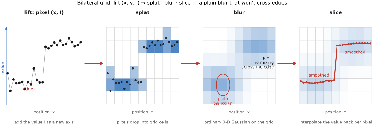
On a single scanline the grid has only two axes, position and intensity, so each step of the pipeline can be followed with its numbers and its cost counted against the brute-force filter (Figure 10.1.11).
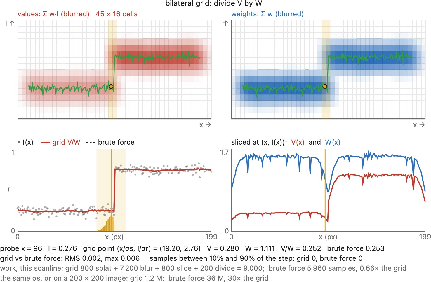
The grid also makes the affinity lesson geometric: the third axis is the affinity, drawn as a coordinate. Two pixels far apart in value are literally far apart in the grid, so a local blur, which only mixes nearby cells, reduces their contribution according to distance and the blur support. The bilateral's "do these pixels belong together?" becomes, in the grid, simply "are these cells close?"
Because the grid is coarse and the blur is a plain convolution, the whole edge-aware filter runs fast enough to be interactive, and the authors put that speed to work on a range of applications.
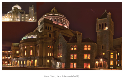
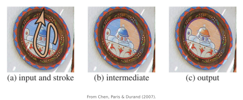

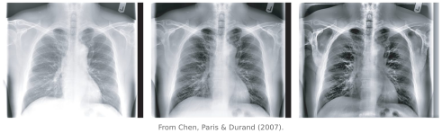
A caveat: the curse of dimensionality. The grid buys speed by coarsening space and range, but its memory grows with the dimension of the cells. A grayscale bilateral needs a 3-D grid (two spatial axes plus one range axis); a color bilateral, or a cross-bilateral keyed on several guide channels, needs a range axis per channel, a 5-D grid for RGB, or more dimensions for additional guide channels whose cell count grows exponentially. And most of those cells are empty: real images occupy only a thin sheet in the space (exactly what the 3-D grid above makes visible: the occupied cells hug the image's intensity surface), so a dense array is enormously wasteful. Andrew Adams and colleagues answer this with the permutohedral lattice (Adams, Baek & Davis 2010 (permutohedral lattice)), a sparse, simplex-based tessellation of high-dimensional space that splats, blurs and slices without allocating a dense Cartesian grid exponential in the feature dimension; runtime still depends on dimension, samples and occupied vertices, making high-dimensional (color, cross-, even non-local) bilateral filtering practical. Read the other way, the bilateral grid is just the low-dimensional, dense special case of this general high-dimensional Gaussian filtering.
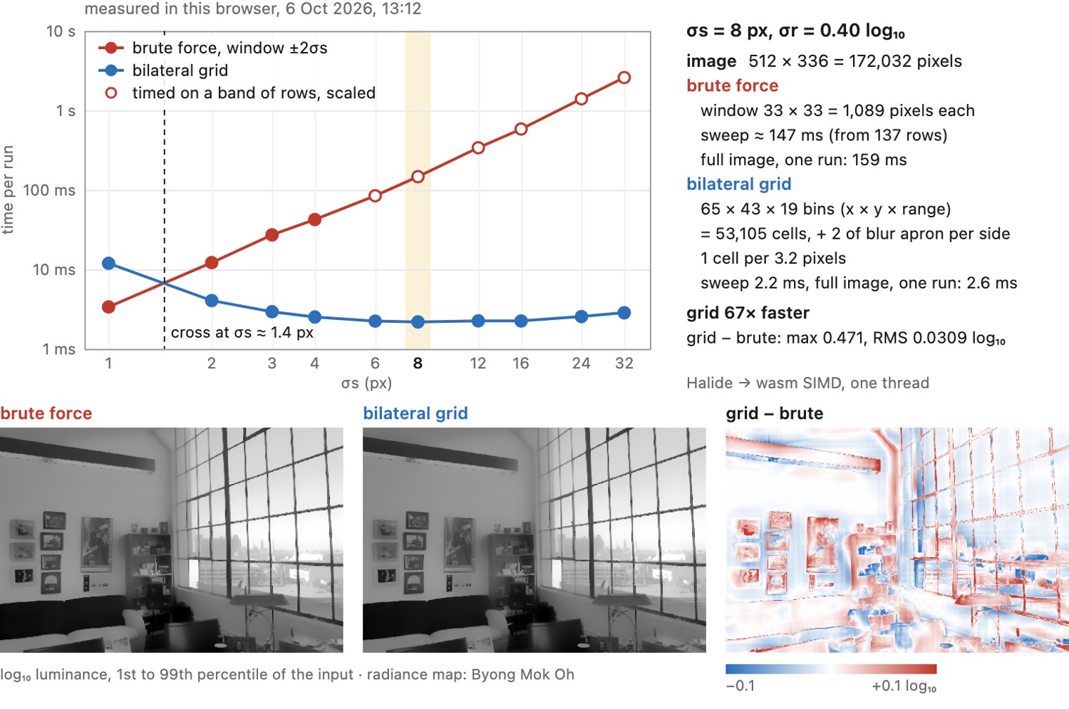
How much the grid saves depends on both widths; timing the two filters on the same image shows where it overtakes the brute force (Figure 10.1.16). The brute force visits a window whose area grows as $\sigma_s^2$, so its cost climbs with the spatial width. The grid's cost does the opposite: a wider $\sigma_s$ means fewer, larger cells, and once the grid is small, what remains is the splat and the slice, which visit every pixel once whatever the widths. With both filters compiled from Halide and run on one thread, the grid overtakes the brute force at a spatial width of only one or two pixels, and at $\sigma_s=8$ it is about 67 times faster on the machine we measured, at a cost of a small error concentrated at strong edges, where the coarse cells blur most.
Bilateral upsampling and learning⧉
optionalMany operations are too expensive to run on a full-resolution photograph: a stereo matcher, an optimization, a large network. A common answer is to run them on a small copy and bring the result back to full resolution. Ordinary interpolation blurs the result across edges, so a depth map or a mask bleeds from the foreground onto the background. The full-resolution image is still available, though, and its edges say where the result should change. The bilateral filter's range weight is the tool for using them, and this section follows that idea from simple upsampling to layers inside neural networks.
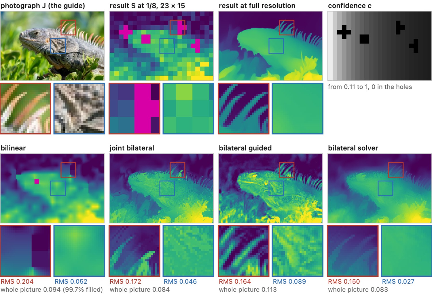
Joint bilateral upsampling. Kopf and colleagues upsample a low-resolution solution $S$ with the full-resolution image as the guide $J$ Kopf et al. 2007 (joint bilateral upsampling). Each output pixel $p$ averages the low-resolution values near its position $p_\downarrow$ in the small image, weighted by distance in the small image and by similarity in the guide:
It is the cross bilateral filter of the previous section with the two inputs at different resolutions. A value from the other side of an edge in the guide gets almost no weight, so the result changes where the photograph does. The guide is not a measurement of the quantity being upsampled, though: a painted stripe is a color edge with no depth edge, and a foreground object the color of its background has a depth edge the guide cannot see. Chapter 29.1, Algorithmic speedups gives the procedure in pseudocode and these failure cases in detail.
Upsampling an operator rather than an image. Chen and colleagues upsample the effect of an operator instead of its output Chen et al. 2016 (bilateral guided upsampling). They run the operator on a small copy of the input and fit, in a coarse bilateral grid, a local affine color transform per cell: the one that best maps the small input to the small output. The grid is then sliced at full resolution, with each pixel's own position and intensity, and the sliced transform is applied to the full-resolution input. Because the transform is applied to the original pixels, the output keeps all of their detail, and the operator only has to get the large-scale changes right. This works for tone adjustments, color grading and many stylizations, anything a smoothly varying color transform can express, and fails for operations that move or create pixels, such as warps or added texture.
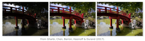
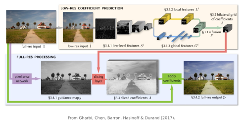
Learning the grid: HDRnet. HDRnet goes one step further and predicts the grid of affine coefficients with a network instead of fitting it to an operator's output (Gharbi et al. 2017, Deep Bilateral Learning). A convolutional network runs on a low-resolution copy of the image and predicts, per grid cell, the coefficients of a local affine color transform. At full resolution the grid is sliced at each pixel's position and at a guide value, itself a learned per-pixel function of the color, and the sliced transform is applied to the pixel. The expensive network stays at low resolution, where it can see the whole image, and the edge-aware slice carries its decision back to every pixel. The bilateral grid becomes a learned, edge-preserving upsampling layer, fast enough to run in a phone's viewfinder (Figure 7.3.4, Figure 7.3.5). Chapter 7.3, Deep learning shows more of its results.
The bilateral solver. Upsampling averages the low-resolution values; some problems instead need to clean them. A network's depth map or segmentation is often noisy, has holes, and comes with a confidence that varies from pixel to pixel. Barron and Poole's fast bilateral solver finds the image $x$ that stays close to a target $t$ where the confidence $c$ is high and is smooth under the bilateral affinity $\hat W$ of the guide everywhere Barron & Poole 2016 (fast bilateral solver):
Solved pixel by pixel this would be a huge system, but the affinity is a bilateral filter, so the problem can be splatted into a bilateral grid, solved there with a small linear system, and sliced back. The solution is differentiable with respect to the target and the confidence, so the solver can sit inside a network and be trained through. It has been used to refine stereo depth, to upsample depth and semantic segmentation, and for colorization.
Trainable edge-aware layers. Two lines of work made the bilateral filter itself a network layer. Jampani, Kiefel and Gehler learned the filter's weights on the permutohedral lattice, the high-dimensional generalization of the grid Adams, Baek & Davis 2010 (permutohedral lattice), instead of fixing them to a Gaussian Jampani, Kiefel & Gehler 2016. Wu and colleagues made the guided filter of Chapter 10.6, Guided image filtering differentiable, with a guide image learned by a small network, so that a network can run at low resolution and be upsampled by a guided filter trained end to end with it Wu et al. 2018 (deep guided filter).
Sharpening segmentations. Semantic segmentation networks produce coarse labels whose boundaries do not follow the objects. A fully connected conditional random field, solved with bilateral filtering in its inner loop, snaps the labels to the image's edges: pixels with similar color and position are encouraged to share a label Krähenbühl & Koltun 2011 (dense CRF). Zheng and colleagues unrolled that inference as layers of a recurrent network so that it could be trained together with the network that produces the labels Zheng et al. 2015 (CRF-as-RNN).
Bilateral grids in neural rendering. Reconstructions of a scene from many photographs, such as neural radiance fields and Gaussian splatting, assume that the same point has the same color in every view. A phone's processing breaks that assumption: exposure, white balance and local tone mapping change from frame to frame, and the reconstruction absorbs the differences as floating artifacts. Wang and colleagues give each view a small learned bilateral grid of affine color transforms, which models that processing and is discarded after training, so the reconstructed scene stays consistent Wang et al. 2024 (BilaRF).
The pattern is the same throughout. A computation too expensive or too coarse for the full image runs at low resolution or on low-quality data, and an edge-aware structure built from the full-resolution image carries the result back, keeping its edges where the photograph's are. What the guide cannot supply is information it does not contain.
Anisotropic diffusion and robust estimators⧉
optionalThe bilateral filter is one member of a family, and the other two members were derived from different starting points and arrive at nearly the same arithmetic. Seeing them together explains what the range weight is really doing.
Read the filter as an estimator first. Averaging a neighborhood is what you do when you believe every neighbor is a measurement of the same value corrupted by Gaussian noise, which is the quadratic penalty $\rho(x)=x^2$. A quadratic grows without bound, so one very different neighbor, the pixel across an edge, pulls the estimate as far as it likes. A robust error norm saturates instead: past some difference a neighbor stops mattering more the further away it is. Edge preservation and outlier rejection are then the same operation, and the bilateral range weight is a particular choice of robust norm (Figure 10.1.18).
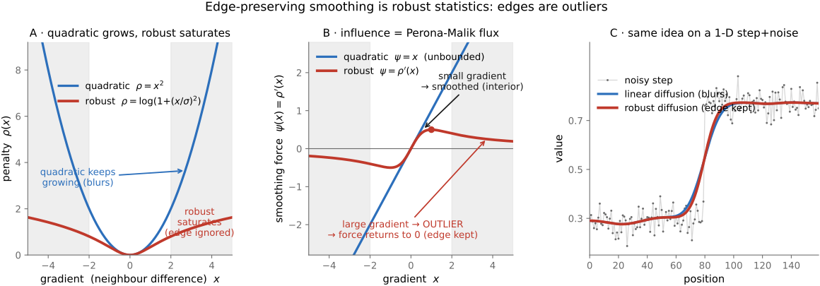
A weighted-difference update resembles one discrete diffusion step. For a symmetric pairwise energy, its force is proportional to the penalty derivative $\psi(t)=\rho'(t)$, while the weight is proportional to $\psi(t)/t$. Weight and influence are therefore different curves: a Gaussian weight yields $\psi(t)=t\exp(-t^2/(2\sigma_r^2))$, up to scale. Perona–Malik diffusion uses a local gradient-dependent conductance Perona & Malik 1990; a finite-neighborhood bilateral update is related but not the same discretization. Some penalties saturate, while others, such as the Lorentzian, grow without bound despite a diminishing influence Black et al. 1998.
Perona and Malik started from diffusion rather than from estimation Perona & Malik 1990. Blurring with a Gaussian is the same as running the heat equation $\partial_\tau I = \operatorname{div}(\nabla I)$ for a time $\tau$ that grows with the blur's variance: intensity flows from brighter to darker neighbors until they agree, across edges as readily as within regions. Their change was to let the flow depend on the local gradient,
with a conductance $g$ near one for small gradients and near zero for large ones, for example $g(s)=1/(1+(s/\kappa)^2)$ or $g(s)=e^{-(s/\kappa)^2}$ with an edge scale $\kappa$. Heat then flows freely inside a region and barely crosses a strong edge, so iterating the equation smooths regions while boundaries survive. Two refinements matter in practice. With these conductances the flux $g(s)\,s$ decreases once $s$ exceeds a value near $\kappa$, so diffusion can steepen an edge rather than merely preserve it, and the continuous equation is ill-posed in that regime; practical schemes measure the gradient on a slightly smoothed image and take explicit time steps small enough to stay stable. A bilateral pass is not a discretization of this equation: it averages over a whole neighborhood in one large step, where diffusion takes many small nearest-neighbor steps.
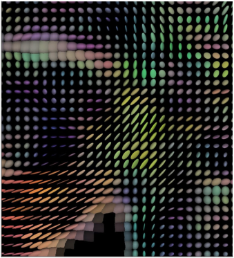
A tensor can express directional diffusion. Diffusion-tensor imaging estimates physical water diffusion from measurements; it is not an image-smoothing algorithm that recovers anatomy by running Perona–Malik.
The practical consequence is that these are three vocabularies for one design decision: how much should a dissimilar neighbor count? The bilateral answers with a range Gaussian, Perona and Malik with a conductance that falls with the gradient Perona & Malik 1990, robust statistics with an influence function. Chapter 13.3, Gaussian, median, and bilateral filtering compares their behavior on noise, and Chapter 10.4, Local Laplacian filters takes the same question to a multiscale decomposition.
Tone mapping and display⧉
optionalOnce we have captured a high-dynamic-range image (often called a radiance map), either using a high-quality sensor or multiple exposures, its range usually exceeds what can be reproduced on a display or print. A scene can span fifteen stops; a good screen or print shows six or seven in good conditions and can be as low as four when stray light lifts the blacks.
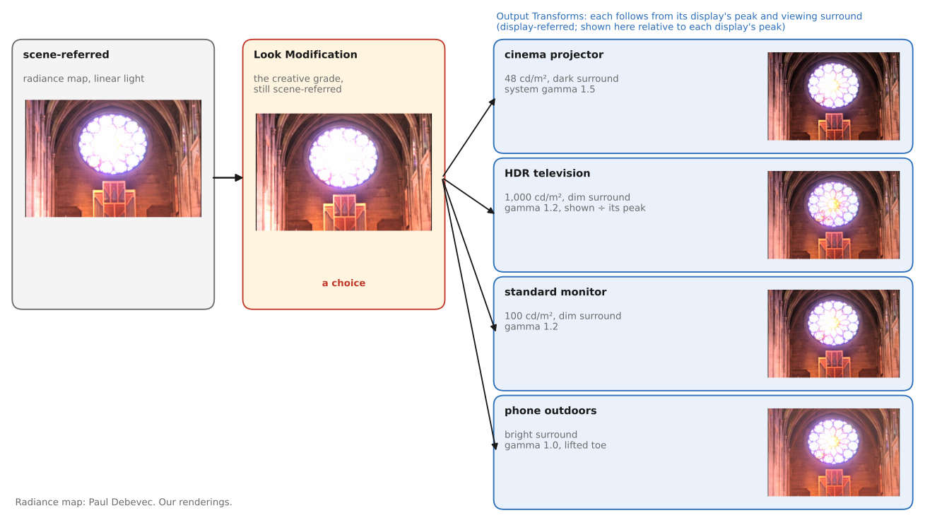
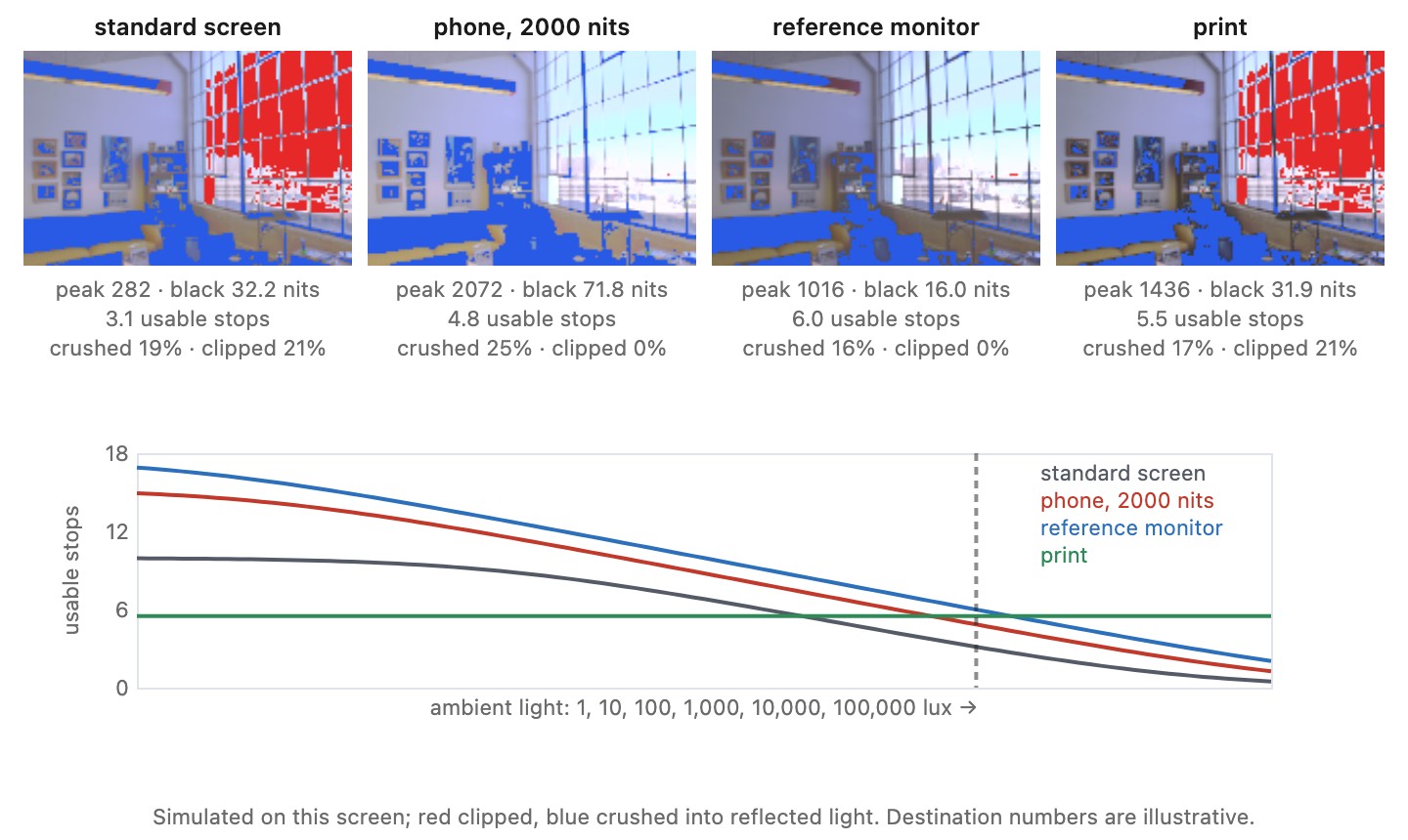
Tone mapping maps values from scene radiance to the final photograph. Imaging pipelines name the two ends. A scene-referred image holds values proportional to the scene's radiance, as a merged bracket does (Chapter 17.7, Encoding HDR images). A display-referred image holds the values a particular display should emit, or a print should reflect. Tone mapping is the step between the two. It is often done without reference to any particular display, aiming at a generic screen or print, although a display is always there implicitly, in the range and contrast the result is designed for. More and more, the display is taken into account explicitly: its peak brightness, its black level and the light of the room it sits in change what the rendering should be (Chapter 5.6, Preparing photographs for viewing, Chapter 18.10, HDR displays and display mapping). Figure 18.0.1 follows one image from the scene-referred state to four displays.
The previous part (Part 17, High dynamic range capture) ends with a measurement and an account of where it is reliable; this part spends it.
Whereas HDR capture is usually an objective measurement proportional to physical units, tone mapping is often a subjective endeavor. In some circumstances, the goals can be tied to psychophysics, especially when realistic simulations are sought. For example, a realistic driving simulation seeks to reproduce visibility properly. But in most photographic situations, the goal is subjective: we want images to look good. Yet, in both cases, knowledge of the human visual system helps set the principles.
Tone mapping and perception⧉
What local tone mapping relies on⧉
optionalThe local methods of the following chapters rest on three properties of spatial vision.
The visual system responds to local contrast far more than to absolute level. Center-surround receptive fields compare a region with its neighborhood, and contrast sensitivity is band-pass: we detect a grating of moderate spatial frequency at much lower contrast than a very slow variation across the visual field (Chapter 3.4, Spatial and temporal vision). A slow gradient of illumination across a room is barely noticed, while a small edge is seen clearly.
Lightness constancy discounts illumination. We judge the reflectance of a surface by comparing it with its surroundings, so a white page in shadow still looks white (Chapter 3.3, Adaptation and constancy). Illumination tends to vary slowly or change abruptly at shadow boundaries, while reflectance carries the texture. Compressing the large-scale variations of a radiance map, mostly illumination, while keeping its local contrast, mostly reflectance, therefore changes what the viewer perceives about the lighting much more than about the surfaces. That is the rationale behind every base/detail method.
The eye adapts locally and moves. Each fixation adapts to a region of the scene a degree or two across, and a viewer scanning a high-contrast scene sees each part at a different adaptation. A local operator is a crude imitation of that process frozen into one image, and the size of the neighborhood it uses plays the role of the adaptation field Pattanaik et al. 1998.
The same properties explain the failures. Edges are where the visual system concentrates its attention: Mach bands (Figure 3.4.1) and the Cornsweet illusion show that it reads contrast at an edge and fills in the regions on either side. A halo, a band of false brightness along a strong edge, is therefore conspicuous, which is why fifteen years of research went into decompositions that respect edges. And because we judge large regions relative to one another, pushing local contrast too far flattens the global relationships, a dark sky ending up as bright as a lit facade, which produces the overprocessed "HDR look".
Global tone mapping⧉
Two families: global and local⧉
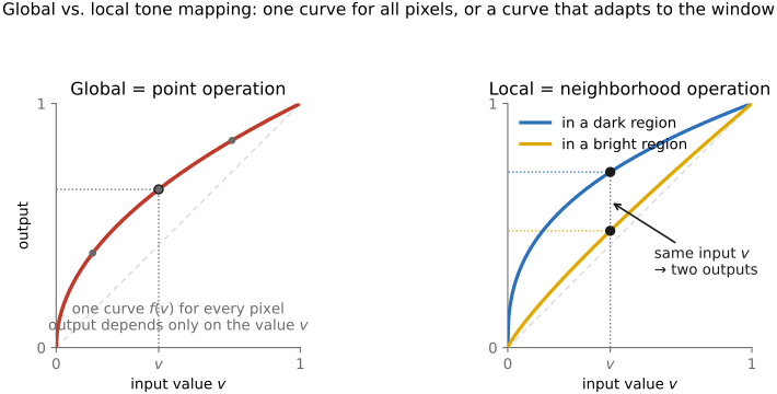
optionalScaling every value by the same factor preserves the scene's ratios, so it cannot by itself make a large range fit a smaller one (Chapter 17.1, Dynamic range and multiple-exposure capture); something has to compress. There are two fundamentally different ways to compress the range, global and local; this chapter covers the first and the rest of the part the second (Figure 18.2.1).
A global tone map applies one function $L_\text{out}=f(L_\text{in})$ everywhere. A monotone scalar curve cannot create a new spatial maximum or minimum, so it does not generate the edge halos caused by a neighborhood filter. It can still reveal existing halos, amplify noise, produce banding after quantization, or alter colors. Compressing a large range reduces contrast over some input intervals.
A global curve redistributes contrast across intensities. For a small difference, $\Delta L_{\rm out}\approx f'(L)\Delta L$. For small relative contrast, the relevant gain is
A compressive log slope below one reduces relative contrast in that intensity range. The curve can allocate more contrast to populated or important ranges and compress others; it need not flatten every detail equally. The same input intensity still receives the same output regardless of its neighborhood.
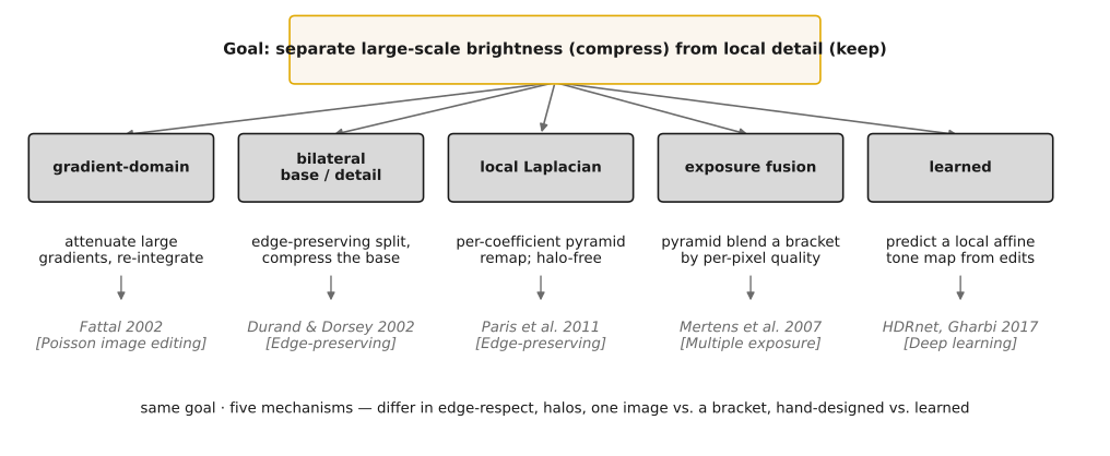
A local tone map adapts to the neighborhood. One construction separates large-scale brightness from detail, compresses the former, and restores the latter. This can preserve texture while reducing the difference between a window and a wall, but the separation can mistake noise for detail and blur across boundaries.
Why log space helps⧉
Log luminance makes relative contrast convenient to manipulate. Scaling a log difference by $c$ changes the corresponding luminance ratio $R$ to $R^c$. For $0<c<1$, this compresses the ratio. Multiplication in linear light is already simple; the benefit here is that ratios become differences that can be separated into base and detail.
This is why the local methods of the following chapters work on log luminance: a base and a detail layer of the log image are a large-scale ratio and a local ratio, and compressing the base compresses large ratios while leaving local ones alone (Chapter 18.3, Two-scale and bilateral tone mapping).
Choose an encoding for the operation. Add independent light contributions in linear light. For relative-contrast decomposition, log luminance turns ratios into differences, so a base and a residual can be combined by addition.
Log luminance is useful when the operation should act on intensity ratios, as in additive base/detail decomposition or gradient attenuation. Other operators, including Reinhard's $L/(1+L)$, can be formulated directly in linear luminance. Match the representation to the operation; do not take logarithms of nonpositive values.
Why a single curve cannot win⧉
optionalAt a given input level, a global curve gives every pixel the same adjustment. If a window and a wall require different treatments at that level, one curve cannot supply them. A local operator can, at the cost of neighborhood-dependent artifacts and more parameters.
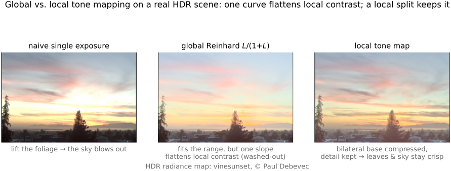
Consider a dark textured wall and a bright textured cloud. A global curve must assign the same output and the same local slope whenever their input values coincide. Flattening a broad part of the curve to fit the scene range also reduces small variations that fall in that part. A local method can treat the wall and cloud differently by using their neighborhoods, but then the transition between neighborhoods becomes part of the problem. The global/local choice trades one consistent mapping for spatial flexibility; it does not make range compression free.
The argument can be made exact with the gain $G(L)$ of the two-families section. A curve that compresses a range of $R$ stops into $r<R$ has an average log-log slope of $r/R$, so over most of the range it must reduce relative contrast, and a small texture at any luminance in that range is reduced along with the large difference that had to be compressed. No choice of shape escapes this, since the curve sees only the value, not whether a variation is the edge of a window or the grain of a wall. Keeping local contrast while compressing the range needs spatial processing: a mapping that depends on each pixel's neighborhood. The rest of the part develops the five ways of doing that (Figure 18.2.10).
Two-scale and bilateral tone mapping⧉
When the range is high, a global curve cannot compress it and keep local contrast at the same time (Chapter 18.2, Global tone mapping). Two-scale methods separate the two jobs. They split the image into a base layer, which carries the large-scale variations and most of the dynamic range, and a detail layer, which carries local contrast and texture; they compress the base and keep the detail. The idea matches what perception allows (Chapter 18.1, Tone mapping and perception): large-scale variations are mostly illumination, which the eye discounts, and local contrast is mostly reflectance, which it reads. This is also the reasoning of Land's Retinex theory of lightness, which estimates the illumination as a smooth version of the image in log space and attributes the rest to the surfaces Land & McCann 1971; its multiscale version was used directly to compress the range of photographs Jobson, Rahman & Woodell 1997 (multiscale Retinex). Everything depends on how the base is computed, and the history of the method is the history of that one choice. The filters themselves are developed in Part 10, Edges matter; this chapter covers their use for tone mapping and the failures they do and do not fix.
Starting with global tone mapping⧉
We start with a simple global tone mapping approach based on a gamma remapping expressed in log values. High-dynamic-range tone mapping is a task where the choice of encoding really matters (Chapter 4.3, Encoding: linear, gamma or log). Working in log luminance, where ratios become differences (Chapter 18.2, Global tone mapping), was recognized decades ago with so-called homomorphic filtering Oppenheim, Schafer & Stockham 1968 (homomorphic filtering), which suggests that when dealing with phenomena that involve multiplications (such as the product of reflectance and illumination), one should work on log values. Log conforms to the visual system's relative invariance to multiplication factors. Any base works, and Durand and Dorsey, like the figures here, use $\log_{10}$. With $Y$ the luminance of the radiance map,
In log values, the multiplicative dynamic range $Y_{\min}:Y_{\max}$ becomes a simple additive range $\log Y_{\max}-\log Y_{\min}$ (Figure 18.3.1, stage input). We can map it to the limited dynamic range of a display (or a target set by the user) $1:\mathrm{DR}$ with a gamma remapping curve (not to be confused with gamma encoding, Chapter 4.3, Encoding: linear, gamma or log; the two are related by the system gamma), with exponent $c$ given by the ratio of output and input dynamic range in log. The gamma exponent becomes a multiplication in log:
Subtracting $\log Y_{\max}$ sends the brightest pixel to $\ell_\text{out}=0$, that is to display white, and the darkest to $-\log\mathrm{DR}$. For a scene of 1:10,000 shown on a display of 1:100, $c=2/4=0.5$.
If we apply this curve to $R$, $G$ and $B$ separately, the colors wash out (Figure 18.3.1, stage per-channel). The exponent pulls every ratio toward one, including the ratios between the channels: a saturated red with $R/G=4$ comes out with $R/G=4^{0.5}=2$ for $c=0.5$, much closer to gray. Chroma and saturation are carried by these ratios, so to preserve them we apply the curve to the luminance alone and put the color back by keeping each pixel's ratios $R/Y$, $G/Y$ and $B/Y$:
The ratios do not change when a pixel is made brighter or darker, which is why they can be held fixed while the luminance is compressed. All of these are linear values; the output still needs the display encoding. Keeping the ratios exactly is a starting point rather than a law of perception, and Chapter 18.2, Global tone mapping discusses its limits and the alternatives.
The colors are now right, but the image looks flat and muddy (Figure 18.3.1, stage luminance). The curve reduces every ratio by the same exponent, small ones as well as large ones: with $c=0.5$ the ratio between the window and the room drops from 10,000 to 100, as intended, and the 2:1 contrast of a texture or of the shading on a face drops to $2^{0.5}\approx1.4$:1. Reducing contrast was the job of the curve, so a global curve cannot avoid it; it cannot tell the large ratios it must compress from the small ones we would like to keep.
Base and detail⧉
The idea of two-scale tone mapping is to apply the gamma contraction only to a large-scale layer of the image, which holds most of the range, and to leave the small-scale variations, which hold the local contrast, untouched. The same idea can be reached from different perspectives. The large-scale layer tells us if a region of an image is bright or dark and we seek to darken bright regions and vice versa, similar to dodging and burning in the darkroom (Chapter 5.5, Developing and editing a photograph; Chapter 18.9, High dynamic range in traditional photography). Or we can view the base as trying to estimate illumination while the detail represents reflectance or albedo variation, and given the human visual system's focus on reflectance, and the limited dynamic range of reflectance, we can afford to compress the contrast of the illumination.
We first attempt to create a base or large-scale layer $B$ using a simple Gaussian blur on the log luminance. The detail $D$ is simply the difference between the original log luminance and the base.
with $G_{\sigma_s}$ a Gaussian of width $\sigma_s$; the methods of the following sections change only this filter. We compress the base with the exponent $c$ and add the detail back unchanged, or amplified by a factor $a$:
The factor $c$ is the exponent of the global curve, now applied to the base alone. We choose it so that the base fits the target output contrast: if the base spans $\Delta B=B_{\max}-B_{\min}$ in log units and the display should show a contrast of $1:\mathrm{DR}$, then $c=\log\mathrm{DR}/\Delta B$. As in the global curve, subtracting $B_{\max}$ puts the brightest part of the base at white; a high percentile is a more robust choice, as in the bilateral method below. With $a=1$ the detail keeps exactly the local contrast it had in the scene; $a>1$ exaggerates it. Color is put back with each pixel's color ratios, as in the global curve.
two_scale_tonemap(Y, rgb, DR, sigma_s, detail_amp=1):
    l = log10(max(Y, eps))
    B = gaussian_blur(l, sigma_s)         # the following sections change only this line
    D = l - B
    c = log10(DR) / (max(B) - min(B))
    l_out = c * (B - max(B)) + detail_amp * D      # brightest base value at 0, i.e. white
    Y_out = 10 ** l_out
    return rgb * (Y_out / Y)[..., None]   # then exposure, gamma or display encoding
With the Gaussian base, smooth regions come out well: the blur averages away the detail and keeps the slow variations, and compressing it leaves the texture intact. The trouble is strong edges. A Gaussian blur does not respect edges: it averages straight across the boundary between the bright window and the dark wall, so near that edge the base is a smeared ramp, too dark on the bright side and too light on the dark side. When we compress this base and add the detail back, the error shows. With $a=1$ the output is $\ell_\text{out}=\ell-(1-c)\,B$ up to a constant, so where the base is too low, on the bright side, too little is subtracted, and where it is too high, on the dark side, too much: next to the edge the bright side comes out brighter still and the dark side darker, a band on each side that exaggerates the edge. This is a halo (Figure 18.3.2; Figure 18.3.1, stage gaussian, follows it on a profile across an edge). It is the same failure mode as naive unsharp masking, and it is the signature artifact of cheap local tone mapping, the glow around the skyline in an over-processed HDR photograph.
This first attempt has a history. Homomorphic filtering, met above, already reduced the slowly varying illumination of the log image with a low-pass filter while keeping the reflectance. The first tone-mapping operator of this kind is Chiu and colleagues' of 1993, and its failure is the most instructive one in this area Chiu et al. 1993. They scaled each pixel by the inverse of a heavily blurred copy of the image, which compresses large-scale variations and keeps the small ones. Where the scene is smooth it works. At a strong edge the blur mixes both sides, and the result is a wide band of false brightness along every high-contrast boundary. The fifteen years of research that followed were mostly about how to compute the large-scale layer without that mixing, rather than about the tone curve applied to it.
An edge-preserving filter reduces mixing across strong boundaries. Its range weights can greatly reduce halos, but do not guarantee their absence; parameter choice, noise, and subsequent clipping still matter. Part 10, Edges matter develops the filtering machinery. Even then, a base/detail decomposition is an approximation, not a unique description of the scene. Large illumination differences often enter the base, while texture and noise enter the residual. Compressing only the base preserves the residual numerically; it does not establish that every preserved variation is useful detail.
Bilateral tone mapping⧉
Durand and Dorsey replaced the diffusion with the bilateral filter, which computes an edge-preserving base in one pass Durand & Dorsey 2002. The bilateral filter averages each pixel with neighbors that are both close in space and close in value (Chapter 10.1, Bilateral filtering). For the log intensity $\ell$, at pixel $p$,
with $f$ a Gaussian of width $\sigma_s$ in space and $g$ a Gaussian of width $\sigma_r$ in log intensity. Near a strong edge the pixels on the far side differ by much more than $\sigma_r$, their range weight is nearly zero, and the average stays on its own side: the base keeps the edge sharp, and the detail layer, the difference between the image and its base, contains no trace of it. Working on log intensity is what makes this right for tone mapping. The range weight then compares ratios, so an edge is "strong" when its contrast is large, whatever the absolute brightness: a window ten times brighter than a wall is excluded from the wall's average in the shadows and in the highlights alike. Since the eye also responds to ratios, the filter's notion of an edge matches the viewer's.
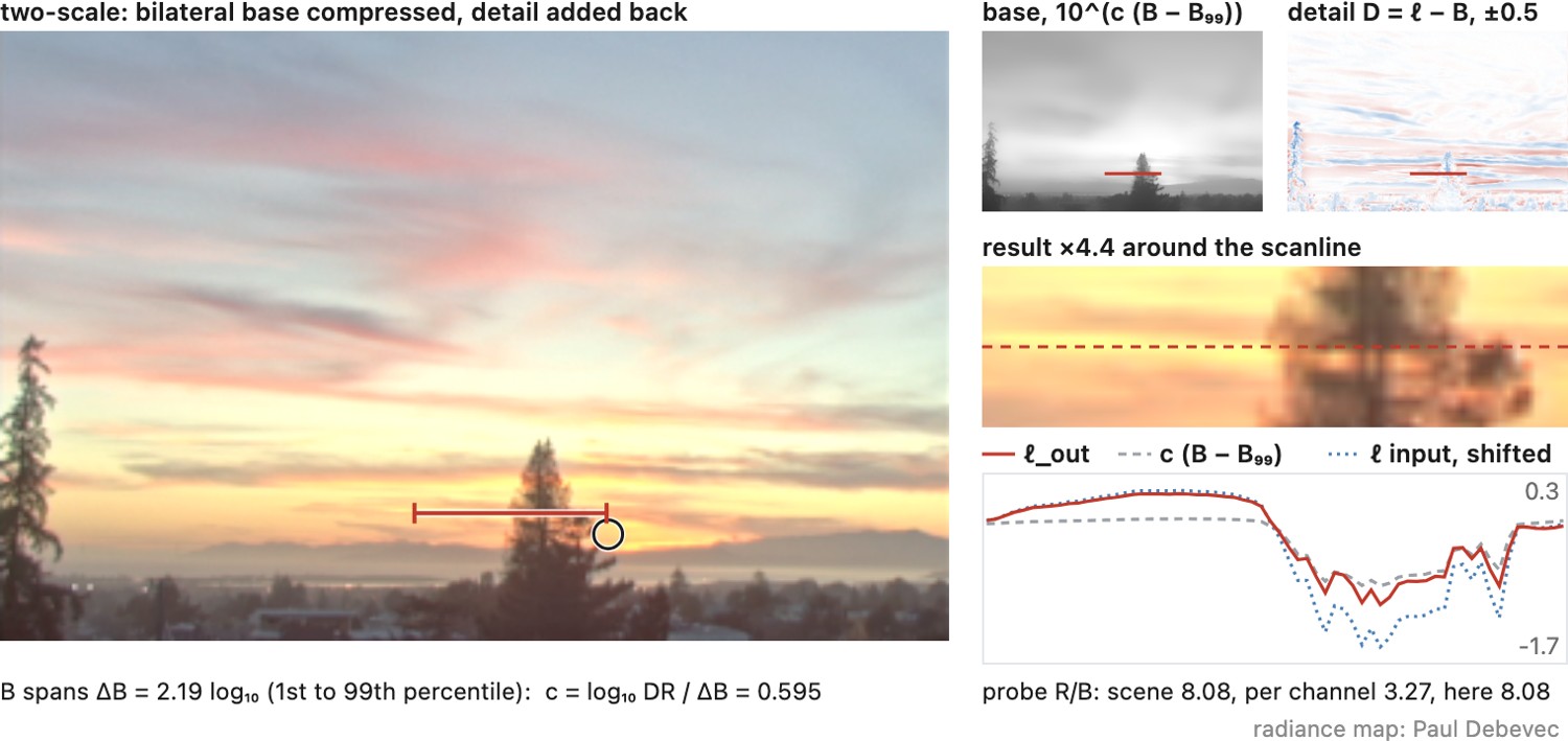
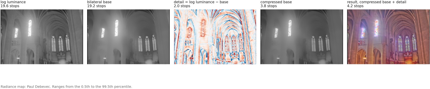
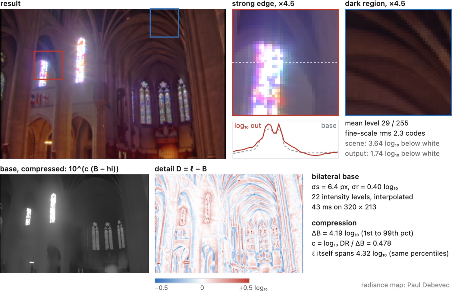
Figure 18.3.3 shows the two layers a bilateral base gives on a real scene.
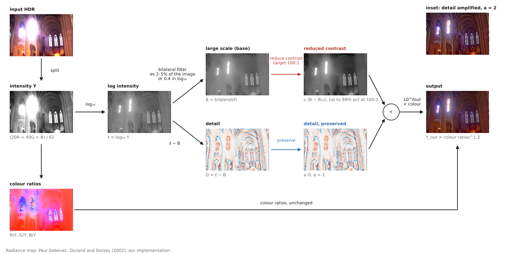
The whole operator follows the diagram of Figure 18.3.4, in six steps.
- Separate intensity and color. Compute an intensity from the radiance map, a weighted sum of the channels; the paper used $Y=(20R+40G+B)/61$, and any luminance will do. Divide the channels by it to get the color ratios $R/Y$, $G/Y$, $B/Y$, which carry the color independently of the brightness. This is the separation of luminance and color met above with the global curve, and for the same reason: compressing $R$, $G$ and $B$ separately would wash out the colors.
- Take the logarithm of the intensity, $\ell=\log_{10}Y$.
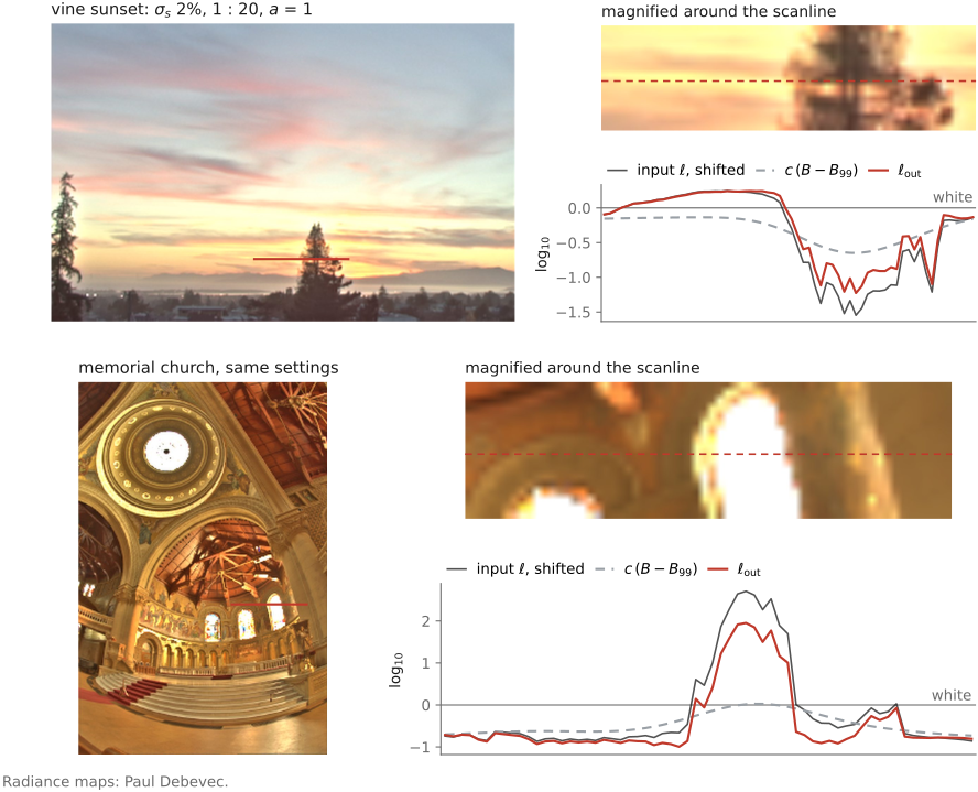
- Compute the base with the bilateral filter, $B=\mathrm{bilateral}(\ell)$. Typical parameters are a spatial width $\sigma_s$ of 2 to 5% of the image size, and a range width $\sigma_r$ of 0.4 in $\log_{10}$, a factor of about 2.5 in intensity.
- Compute the detail, the residual $D=\ell-B$.
- Compress the base. Choose the contrast $1:\mathrm{DR}$ the base should have on the display, for instance 1:100. The base spans $B_{\max}-B_{\min}$ in log units, so the compression factor is $c=\log_{10}\mathrm{DR}/(B_{\max}-B_{\min})$. The output log intensity is
where subtracting $B_{\max}$ puts the brightest part of the base at zero, that is at white, and $a$ is the detail amplification, one to keep the detail as it was. In practice the extremes are better taken as percentiles, the 1st and 99th for instance, so that a few hot pixels or specular points do not set the scale for the whole image, as Figure 18.3.4 and the explorer of the next section do.
- Recombine. $Y_{\rm out}=10^{\ell_{\rm out}}$, and each channel is $Y_{\rm out}$ times its color ratio. The result is display-linear and still needs the output encoding.
bilateral_tonemap(R, G, B, sigma_s=0.02*width, sigma_r=0.4, DR=100, detail_amp=1):
    Y = (20*R + 40*G + B) / 61                    # intensity
    r, g, b = R/Y, G/Y, B/Y                        # color ratios, independent of brightness
    L = log10(Y)
    base = bilateral(L, sigma_s, sigma_r)          # edge-preserving large scale
    detail = L - base                              # residual: texture and local contrast
    hi, lo = percentile(base, 99), percentile(base, 1)   # robust max and min
    c = log10(DR) / (hi - lo)                      # compress the base to the target contrast 1:DR
    L_out = c * (base - hi) + detail_amp * detail  # bright end of the base at 0, i.e. white
    Y_out = 10 ** L_out
    return Y_out*r, Y_out*g, Y_out*b               # then gamma or the display's encoding
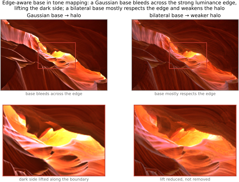
On the sunset, the bilateral base removes the halo of the Gaussian one (Figure 18.3.1, stage bilateral).
What matters. The method has few parameters, and they do not matter equally. The spatial width $\sigma_s$ is not critical: anything from about 2 to 5% of the image size gives similar results, because it only has to be larger than the texture and smaller than the regions. The range width $\sigma_r$ matters much more. Too small, and moderate texture counts as edges, so it stays in the base and is compressed; too large, and strong edges are averaged across, and the halos of the Gaussian base return. The log domain is essential, for the two reasons above: the scene's range is too large for a range weight on linear values to make sense, and contrast is perceived as a ratio. The choice of intensity is less critical but changes the result; a better function of the channels can help, as in the flash and no-flash work that followed Eisemann & Durand 2004. Figure 18.3.6, in the next section, lets the reader vary both widths.
Detail amplification. With $a>1$, the detail layer is amplified: textures and small contrasts become more pronounced than in the scene. In moderation this restores the local contrast that viewers expect from a print; pushed far, it produces the overprocessed look discussed below.
A single image. The operator does not need a bracket. A raw file from a modern camera holds 12 to 14 stops (Chapter 17.1, Dynamic range and multiple-exposure capture), more than a display shows, and benefits from the same compression; shadow-lifting tools in raw developers are close relatives. The limit is noise: lifting the base of a dark region raises its noise along with its detail, since the detail layer contains both.
Speed. Computed directly, the bilateral filter is slow: each pixel averages a large neighborhood with weights that depend on the pixel itself, so it cannot be done as a convolution, and on the images of 2002 a direct implementation took minutes. Durand and Dorsey made it fast by linearizing it. They chose a small set of intensity levels; for each level, the range weight is a fixed function of the pixel values, so the weighted sums $\sum_q f\,g\,\ell_q$ and $\sum_q f\,g$ become ordinary convolutions, computed with fast Fourier transforms and at reduced resolution; each pixel then interpolates the result between the two levels nearest its own intensity. This piecewise-linear acceleration was the first step toward the bilateral grid, which treats intensity as a third dimension, splats the image into a coarse three-dimensional grid, blurs it and reads it back, and runs in real time on a graphics processor Paris & Durand 2009 Chen et al. 2007 (Chapter 10.1, Bilateral filtering).
The decomposition zoo, and what it fixes⧉
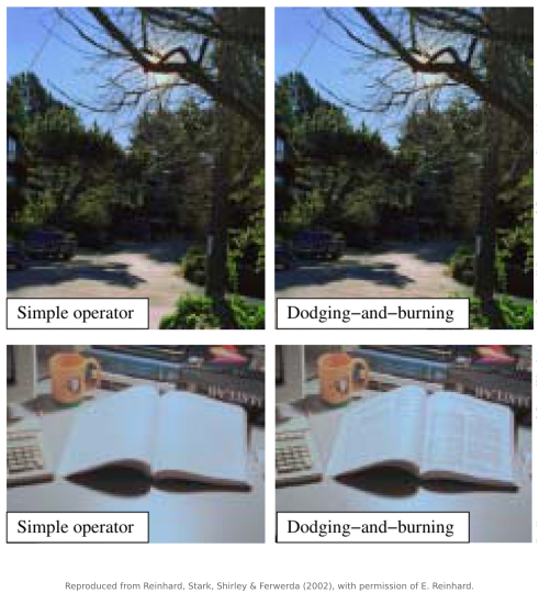
optionalReinhard and colleagues reached an edge-aware base from the darkroom side. Their automatic dodging-and-burning chooses, at each pixel, the largest neighborhood over which the image is roughly uniform, by comparing blurs at successive scales and stopping before one straddles a strong edge, and uses that neighborhood's average as the local adaptation level Reinhard et al. 2002. The per-pixel scale selection is an edge-aware base by another route.
After the bilateral filter, many edge-preserving smoothings were proposed as better bases, each developed in Part 10, Edges matter. The weighted-least-squares smoothing of Farbman and colleagues solves for a base that stays close to the image while being smooth except where the image gradient is large, and supports a multiscale split into several detail layers; at a large spatial scale it lets a bright window's glow return Farbman et al. 2008. The guided filter computes a locally linear fit to a guide image and is fast and free of the bilateral's gradient reversals, though it softens a strong step slightly, by about a tenth in the explorer below He, Sun & Tang 2013 (guided filter) (Chapter 10.6, Guided image filtering). The bilateral grid makes the bilateral real-time on a graphics processor Chen et al. 2007, and HDRnet learns to predict local affine tone adjustments in such a grid from examples (Chapter 18.8, Display rendering transforms and color).
They differ in what they fix. Edge-aware bases greatly reduce halos at strong edges, but none removes them everywhere: an edge with a moderate contrast, close to the filter's range scale, is partly smoothed, and a soft halo remains. The bilateral filter can produce gradient reversals, thin bright or dark lines along edges that a smooth ramp should have crossed, because it treats a pixel on a ramp as an outlier; the weighted-least-squares and guided filters reduce them. None of them fixes noise. The detail layer contains the sensor noise along with the texture, and when the base of a dark region is raised while its detail is kept, the noise there is raised in relative terms; denoising before tone mapping, or limiting detail gain in dark regions, is part of a working pipeline. And none fixes the look. A detail gain above one, or a base compressed too far, flattens the large-scale relationships of the scene, the dark sky that ends up as bright as the lit facade, which is the overprocessed look of many HDR photographs of the 2000s. That is a choice of parameters, not a failure of the filter.
Figure 18.3.6 puts the four bases side by side on one radiance map, with the halo and the noise each under a magnifier.
HDR displays and display mapping⧉
What a display can actually show⧉
optionalA rendered HDR image must pass through a file format, decoder, color-management system and display. A capable panel alone is insufficient if an intermediate step strips the metadata or converts the image to standard range.
Peak luminance depends on bright-area size, duration and power limits. Visible black depends on panel emission, leakage and reflected ambient light. Some reference values give a sense of scale. Standard-range video is mastered for a reference white of about 100 cd/m², and the sRGB reference display is 80 cd/m². ITU-R BT.2408 places the reference white of HDR content at 203 cd/m², leaving the range above it for highlights. PQ encodes luminances up to 10,000 cd/m²; mastering monitors commonly reach 1,000 cd/m² or more, and recent phones advertise peaks above 1,000 cd/m² for small bright areas. Those conditions matter as much as the nominal peak; two displays with the same advertised brightness can render the same image differently (Chapter 5.6, Preparing photographs for viewing).
Evaluating tone mapping⧉
Why the comparisons disagree⧉
optionalTwenty years of comparison studies have not produced an agreed ranking of tone-mapping operators, and the reason is less the difficulty of running experiments than the question they ask. Kuang and colleagues compared eight operators by paired comparison and found Durand and Dorsey's bilateral operator and Reinhard's photographic operator best overall Kuang et al. 2004. Ledda and colleagues compared six operators against the same scenes shown on a high-dynamic-range display, and declined to rank them at all Ledda et al. 2005. Yoshida and colleagues had observers compare operators with the real scenes, viewed in place Yoshida et al. 2005. Čadík and colleagues rated operators on separate attributes, brightness, contrast, detail, color and artifacts, and related those to overall quality Čadík et al. 2008. These studies asked about preference, about fidelity to a displayed reference, about fidelity to the real scene, and about attributes; there is no reason their answers should agree. "Which operator is best" is underdetermined until we say which of the goals of Part 18, Tone mapping and display we mean: fidelity to the scene's appearance, maximum visibility of detail, or preference. And most of these studies ran each operator at its default parameters, while a single operator's own parameter can move its result further than the differences between operators (Figure 18.11.1).
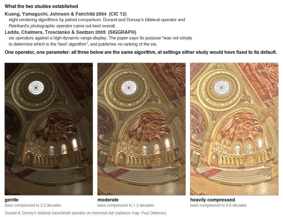
Defaults are appropriate for comparing out-of-the-box behavior. For claims about algorithmic capability, specify a fair tuning budget and evaluate the frozen configurations on separate images. Report the settings and test whether the conclusion changes over a reasonable parameter range.
There is no ground truth for the third goal, and only an expensive one for the second: an appearance match needs the scene, or a display that reproduces it, beside the result. Objective metrics fill part of the gap. HDR-VDP models early vision, from the optics of the eye through contrast sensitivity at several scales, and predicts whether a difference between a reference and a test image is visible and how much it degrades quality Mantiuk et al. (HDR-VDP). It needs absolute, calibrated luminances and a description of the display. It tells whether a difference can be seen, not whether it is better: it cannot express preference, it does not model the appearance effects of Chapter 18.1, Tone mapping and perception beyond contrast visibility, and a tone-mapped image, which is supposed to differ visibly from its HDR input, is not what it was built to judge. Metrics designed for tone mapping, such as TMQI below, combine structure with a statistical model of naturalness for that reason.
Calibrated HDR scenes for tone-mapping evaluation; Google's RAW burst set behind HDR+ Hasinoff et al. 2016. <http://markfairchild.org/HDR.html> · <https://hdrplusdata.org>. See the Chapter 45.16, Datasets appendix.
Recap: big lessons in this lecture
Shared multiplicative changes preserve ratios and often leave surface appearance approximately stable. Brightness, visibility, and color can still change. Gain-control models are useful within their assumptions; they do not make vision insensitive to illumination.
Dividing a value by a similarly scaled reference cancels a common multiplier. Taking logarithms turns the ratio into a difference. This explains why log coordinates are useful for relative changes, without claiming that vision uses a global logarithm or that HDR storage requires one.
The eye is not equally sensitive to every spatial frequency. Luminance sensitivity is band-pass, peaking at a few cycles per degree and falling away on both sides, and the curve moves with light level, field size and contrast. It is defined per degree of visual angle, not per pixel, so viewing distance and display size decide which frequencies a reader can resolve at all. Quote a peak from a textbook and you have described one experiment's conditions; measure it in the conditions you ship in.
Use the color / intensity difference between two pixels as how much they belong together, an affinity, then average (or connect) pixels in proportion to it. Pixels with high affinity are treated as measurements of the same underlying thing and get averaged together; pixels with low affinity, across an edge, are kept apart. The bilateral filter's range weight $g_r$ is the first full instance, but the same affinity drives the bilateral grid, the guided filter, non-local means (NL-means), colorization, and matting / segmentation that follow. Edge-preserving is affinity. (This is L10.1, registered in Part 13, Denoising where the bilateral first appeared for noise; this is its full edge-preserving treatment.)
Removing the bilateral normalizer changes the filter. Specify a normalized spatial kernel or an explicit step size, then test constants, impulses and edges. A small total affinity makes a small correction; it does not establish that an isolated value is correct.
The bilateral is awkward because it is non-linear: its weights depend on the pixel values, so they differ at every output pixel and the filter is not a convolution. The bilateral grid's deeper trick, beyond "add a dimension", is to discretize the intensity (range) axis into a small set of levels, and then do cheap, ordinary linear work at each level. Quantize $I$ into grid layers, run a plain blur within and across layers (distant layers interact less, with accuracy controlled by grid resolution and the blur), and interpolate back to each pixel's exact value. The per-pixel nonlinearity becomes "a few linear passes plus a lookup." This is a general recipe, not a bilateral-only hack: the fast local Laplacian filter (Chapter 10.4, Local Laplacian filters, Aubry et al. 2014) accelerates its per-pixel nonlinearity the same way: evaluate a handful of discrete intensity levels of a slow operator and interpolate between them. Whenever a filter's cost comes from a continuous, value-dependent response, discretizing that response axis turns it into reusable, parallel, convolution-shaped work. (Registered in Big Lessons as L10.2; recurs in Chapter 10.4, Local Laplacian filters and, as an algorithm-level speedup, in Chapter 29.1, Algorithmic speedups.)
Lifting the image into the higher-dimensional grid $(x, y, I)$ is what makes the coarse grid safe. Because pixels on opposite sides of an edge sit at different intensity heights, they are already separated along the range axis, so you can downsample the spatial axes aggressively while retaining range information that ordinary spatial downsampling would lose; coarse sampling can still distort boundaries. Two gains follow: high-resolution edges survive despite a coarse grid; and a large spatial kernel becomes a small blur on the coarse grid, so larger spatial widths may reduce grid work, although full-resolution splatting and slicing still cost at least one pass over the image. Paying one extra dimension for cheap, edge-aware, large-scale smoothing is a trade that recurs: NL-means' patch space, the permutohedral lattice, and the learned bilateral grid (HDRnet) below all live on it.
Choose an encoding for the operation. Add independent light contributions in linear light. For relative-contrast decomposition, log luminance turns ratios into differences, so a base and a residual can be combined by addition.
Log luminance is useful when the operation should act on intensity ratios, as in additive base/detail decomposition or gradient attenuation. Other operators, including Reinhard's $L/(1+L)$, can be formulated directly in linear luminance. Match the representation to the operation; do not take logarithms of nonpositive values.
Defaults are appropriate for comparing out-of-the-box behavior. For claims about algorithmic capability, specify a fair tuning budget and evaluate the frozen configurations on separate images. Report the settings and test whether the conclusion changes over a reasonable parameter range.