Lecture Notes 5 — Demosaicking⧉
Course notes cut from Computational Photography, an AI-powered Slopendium for this lecture. Each section links back to its home in the book; sections marked optional go beyond what the lecture needs.
Contents · 27 sections on this page, from 12 chapters of the book
Titles jump to the section below; ↗ opens it in the book.
Sensing color: multiplexing strategies⧉
A bare photosite usually reports one integrated charge measurement, with a wavelength-dependent quantum efficiency, so to capture color we must somehow take three (or more) measurements where a given photosite provides only one. Every color camera multiplexes those measurements across some axis, and there are several ways to do it, each spending a different axis (Figure 4.6.1).
Strip away the color filter and a sensor is monochrome at the pixel: each photosite reports a single number, a signal proportional to detected photoelectrons within its operating range, not a color. The three (or more) values that color needs must therefore be multiplexed along some other axis: over space (a color-filter array such as Bayer, paying with resolution and a demosaicking step), over time (sequential color filters, paying with motion robustness: the old color-wheel and many scientific cameras), across multiple sensors (a beam-splitter prism feeding three chips, the 3-CCD video camera, paying with bulk and cost), or over depth (wavelength-dependent absorption in stacked photodiodes, the Foveon, paying with noise). The choice determines which measurements are simultaneous and co-located. The same constraint shapes the eye, whose three cone types sample color over space at the retina (L3.1, L3.6).
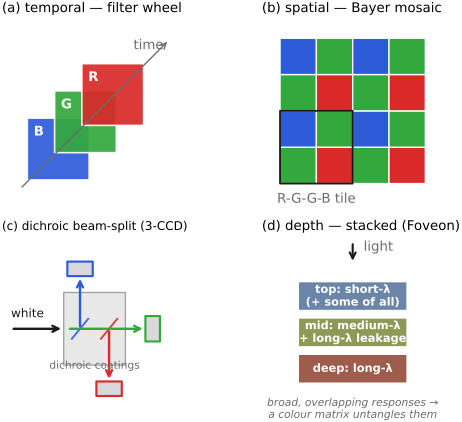
Three-channel color requires three distinct spectral measurements. Distributing them across space or time introduces assumptions about how the scene varies. Multiplex in time and you must assume the scene holds still between frames; multiplex in space and you must assume color varies smoothly enough to interpolate the samples you skipped; multiplex in depth and you inherit badly overlapping bands you then have to un-mix. A beam-splitter can send co-located, simultaneous images to several sensors, at the cost of alignment and optical complexity. A nanoscale router that sends wavelengths to neighboring photodiodes still uses spatial sampling.
Multiplexing in time⧉
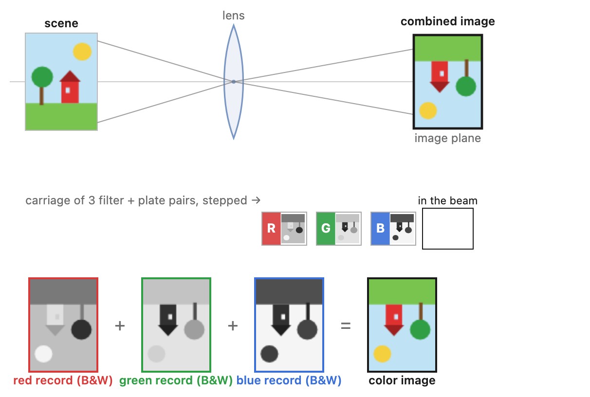
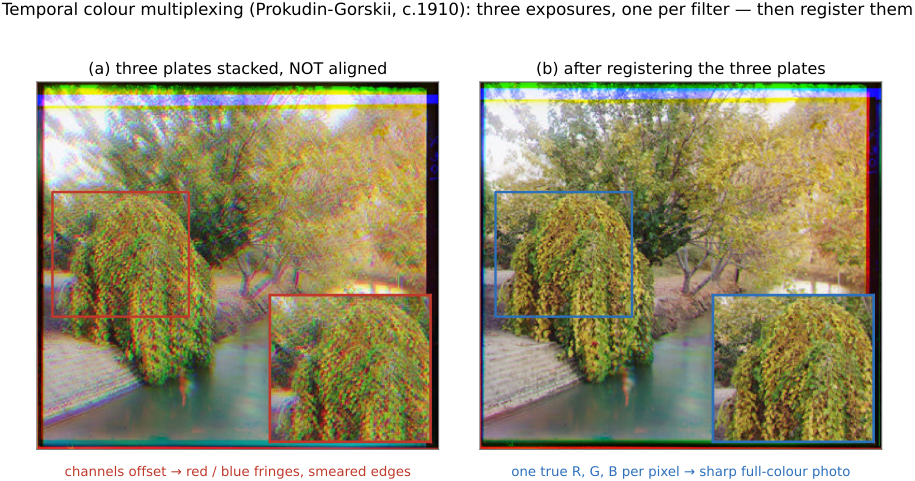
optionalShoot red, green, and blue frames sequentially through colored filters, or a rotating filter wheel. This is the principle behind Maxwell’s early color-photography demonstration (Maxwell 1861) and how Prokudin-Gorskii (Prokudin-Gorskii) captured the Russian Empire in three exposures. It is still how flatbed scanners, astronomy and fluorescence-microscopy filter wheels, telescope narrowband imaging, sequential-color machine-vision cameras, and many multispectral instruments work, because the same mechanism extends naturally from three filters to tens of narrow bands.
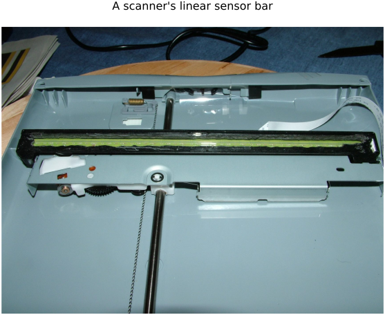
The implementations differ mainly in what does the sequencing. The oldest is a rotating filter wheel (or three separate plates) in front of a single sensor: three exposures through red, green, and blue filters, combined afterward. Maxwell’s 1861 tartan-ribbon demonstration and Prokudin-Gorskii’s later survey are early examples. Astrophotography still leans on it heavily: a cooled monochrome sensor (a mono sensor avoids the color filter array's light loss and keeps full resolution) sits behind a motorized filter wheel and stacks many long sub-exposures through each filter, red / green / blue for natural color or narrowband hydrogen, oxygen, and sulfur filters for nebulae, with tracking and registration to account for camera and celestial motion. Many flatbed scanners also scan spatially over time: a sensor bar is swept mechanically down the page, which is itself how a one-dimensional line sensor becomes a two-dimensional image (scanning spends time to buy the spatial axis the sensor lacks), and color can come from sequential illumination during a scan, separate passes, or spatially offset filtered sensor rows. Field-sequential color television and some endoscopes ran the same spinning-color-wheel trick in real time.
The trade-off is discrimination in time: the method assumes the scene and camera hold still across the exposures. For a static scene, each band uses the full sensor grid. The filters still reject light, and a fixed total capture time must be divided among bands. If the scene moves, its changing parts splits into colored fringes (Figure 4.6.6), and every temporal system must first register the plates to undo the small shifts between them (Figure 4.6.5), the simplest image-alignment problem in the book.
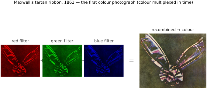
The three-color principle was demonstrated in 1861 by James Clerk Maxwell, the physicist who also unified electricity, magnetism, and light into the equations that bear his name. To demonstrate three-primary additive color reproduction, he had the photographer Thomas Sutton shoot a tartan ribbon three times through red, green, and blue liquid filters, then projected the three black-and-white positives back through the same three filters, superimposed, onto a screen. The overlap showed color in the celebrated 1861 demonstration, and a live demonstration of trichromacy, the same three-number logic the rest of this book rests on. It very nearly should not have worked: the wet-collodion plates of the day were almost blind to red and green, and the "red" record came mostly from ultraviolet that the ribbon's red dye happened to reflect. A lucky accident, but the principle was exactly right, with limitations imposed by the plates’ spectral sensitivity. (Maxwell 1861)
Multiplexing in space: the color filter array⧉
The dominant choice by far. Lay a color filter array (CFA) directly over the sensor so each photosite records one color and the missing two are filled in afterward by demosaicking (Figure 15.0.1, at the start of Part 15, Demosaicking and joint methods). The archetype is the Bayer mosaic, two green photosites for each red and blue, its doubled green mirroring the eye's green-weighted luminance (the eye is itself a spatial CFA, its interleaved cone mosaic). The family is large: Fujifilm’s X-Trans uses a repeating $6\times6$ tile that redistributes sampling artifacts; it does not eliminate aliasing; complementary CMY or CYGM (cyan-yellow-green-magenta) arrays pass more light through each filter than the primary RGB dyes; RGBW arrays add an unfiltered panchromatic "white" pixel for low-light sensitivity; and Huawei's RYYB swaps green for yellow to gather still more light. Phone sensors with many small pixels also group same-color photosites under one filter color. Quad-Bayer puts each color on a 2 × 2 block of photosites, and Nona-Bayer (Samsung's Nonacell) on a 3 × 3 block, so that a 108-megapixel sensor can combine each block of nine into one photosite and deliver a 12-megapixel image with less noise in low light, or read every photosite in good light. Chapter 15.5, Alternative color filter arrays covers how these layouts are demosaicked.
The reconstruction uses spatial and cross-channel regularity to estimate missing samples. Fine colored detail can violate those assumptions, producing false color and zipper artifacts. An optical low-pass filter can reduce aliasing at the cost of detail; not every camera uses one. A CFA also loses photons in its absorbing filters. Its practical advantage is simultaneous capture on one compact sensor.
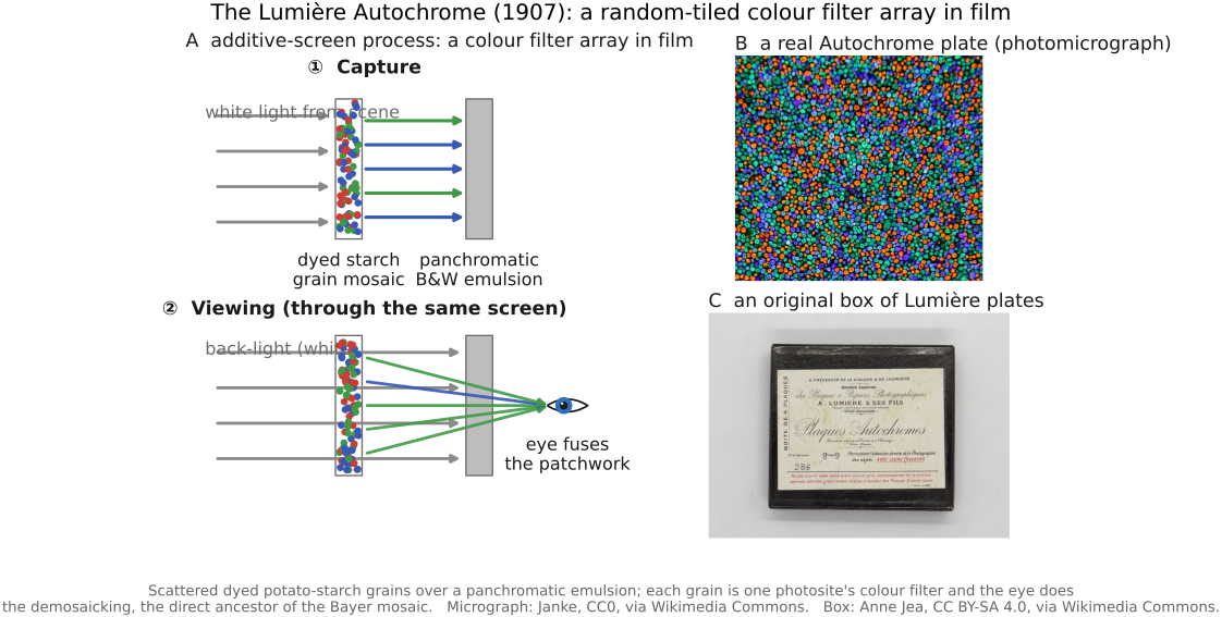
Color film reached the same spatial idea decades before silicon, by literally the same trick. The additive screen processes, the Lumière brothers' Autochrome (1907) and later Dufaycolor, Finlay, and Paget, coated the plate with a fine mosaic of transparent grains or patterned filters (Autochrome used orange-red, green, and violet-blue potato-starch grains; Dufaycolor printed a regular réseau grid) over a single panchromatic black-and-white emulsion. Each grain passed only its own color to the silver behind it, so the developed plate, viewed back through the same mosaic, rebuilt color from a spatial patchwork of filtered samples. This is a color filter array in film, the direct ancestor of the Bayer mosaic, decades before electronic CFAs, with each dyed grain filtering the emulsion behind it and vision integrating the fine mosaic at viewing distance. (The other film tradition, the stacked-dye integral tripack of Kodachrome and modern color film, multiplexes color in depth instead, and so belongs with the Foveon below.)
Multiplexing across separate sensors: the beam-splitter⧉
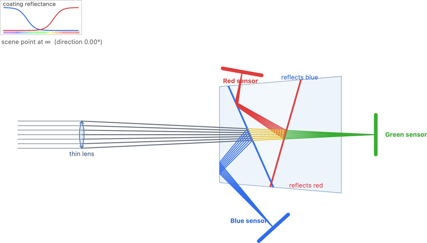
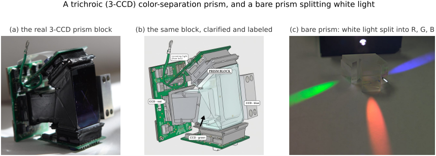
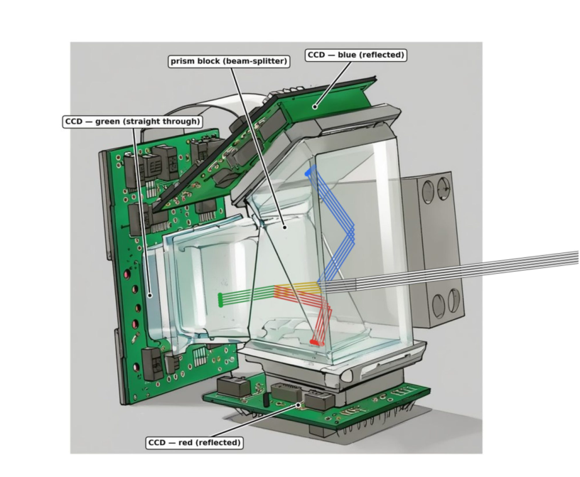
optionalSend the whole image to more than one sensor and give each its own color. A dichroic prism block reflects each band onto its own chip (Figure 4.6.10): the 3-CCD / 3-chip design long standard in broadcast video cameras, three-chip cinema and telecine cameras, and scientific and machine-vision multi-sensor rigs. Because the dichroic coatings split the light rather than absorb it, the separation can retain more useful light than absorbing filters, and each channel has its own full sensor grid. (It is a dichroic beam-splitter, not a dispersing prism: it peels off three clean bands, it does not smear a spectrum.)
This strategy spends no scene axis, so it makes none of the constancy or smoothness assumptions of the other two: simultaneous sampling on three full grids without CFA demosaicking. Instead you pay hardware complexity: three sensors registered to sub-pixel accuracy behind a bulky, expensive prism. Bulk, optical tolerances, and cost limit its use. Adding bands increases the complexity.
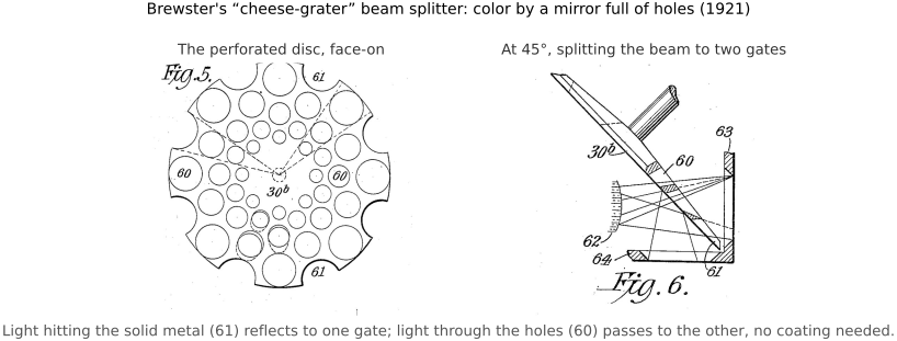
The hardware-splitting idea predates its dichroic form. Before interference coatings existed, P. D. Brewster’s historical beam splitter divided a movie camera's beam with a polished metal disc drilled full of holes (Figure 4.6.8): light passing through the holes went straight to one color film gate, while light striking the solid metal between them reflected off to a second. It is the cheese-grater ancestor of the 3-CCD prism, the same bargain of spending hardware rather than a scene axis so that each color gets its own sensor. It was cruder in two ways: the fixed metal-to-hole ratio sets a single reflect/transmit split rather than a wavelength-selective peel, and because the disc splits by geometry and not by color, each path still needs its own color filter. So it lacks the dichroic prism's wavelength-selective separation, but the core move is identical.
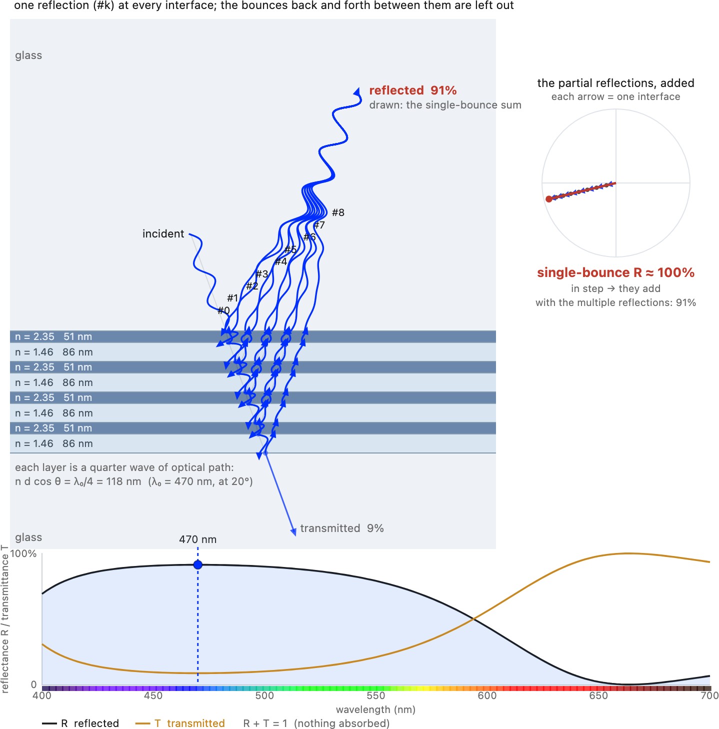
A dichroic coating separates bands through interference. The answer is the same interference that colors a soap bubble (Figure 2.1.33), run deliberately and many times over. The coating is a quarter-wave stack: alternating layers of a high- and a low-index transparent material, each with optical thickness $n_jd_j=\lambda_0/4$ at normal incidence in the simple quarter-wave design. Every interface reflects a little, and at $\lambda_0$ those weak reflections all come back in phase and add into a near-perfect mirror; outside the reflection band the coating transmits more light, with the detailed spectrum set by its complete layer design. In an ideal lossless coating, reflectance plus transmittance is one. Real stacks also have absorption, scattering, angular dependence, and polarization dependence (Figure 4.6.9).
Multiplexing per pixel by dispersion: color routers and nano-prisms⧉
optionalA color router directs wavelength bands toward different photodiodes instead of rejecting unwanted bands with absorbing filters. Demonstrations range from dielectric splitters Nishiwaki et al. 2013 to inverse-designed structures Zou et al. 2022. The target is better photon utilization, but reported efficiency depends on wavelength, incidence angle, polarization, aperture, and the definition of useful detector area. One-third transmission is a teaching approximation for idealized equal-width RGB filters, not a universal CFA ceiling.
Routing to neighboring photodiodes still multiplexes color in space. The spatial response must be included in reconstruction; spreading light is not automatically a correctly designed anti-aliasing filter. Fabrication tolerances and off-axis response also matter. Commercial microlens or nanostructure enhancements that retain color filters should be distinguished from filter-free research routers.
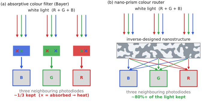
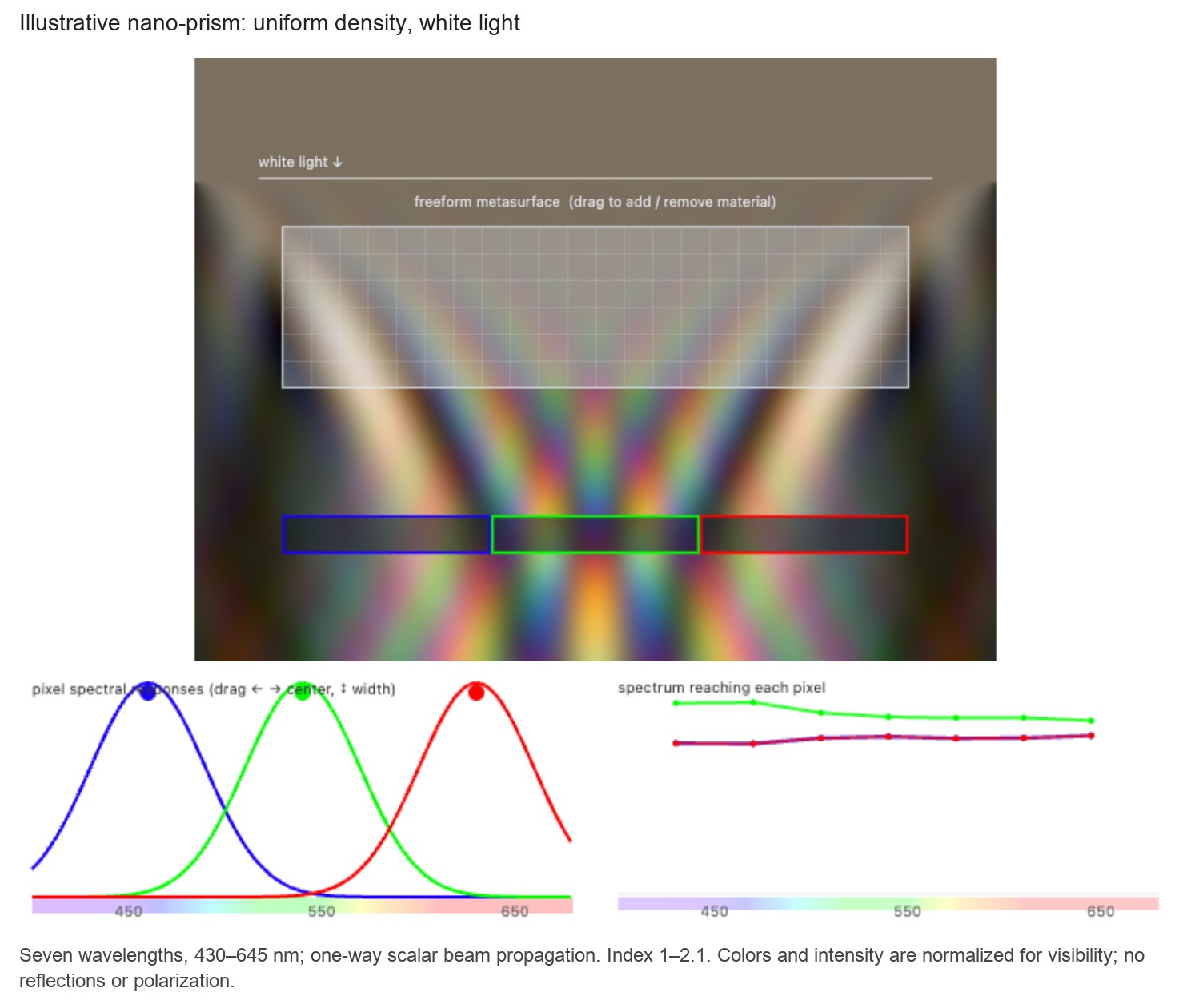
The comparison with a dichroic prism is useful, provided we keep track of the image coordinates. A prism can send complete registered images to separate sensors. A small router sends different wavelengths toward different sites within a local footprint. The latter can avoid absorbing some of the photons that a dye would reject, but neighboring detectors now receive contributions shaped by the router's wavelength-dependent spatial response. The reconstruction must know both which wavelengths and which scene locations contributed. Improving light collection and preserving spatial detail are therefore coupled design tasks, not two independent benefits of replacing a filter.
Multiplexing per pixel by tunable absorbers: quantum dots⧉
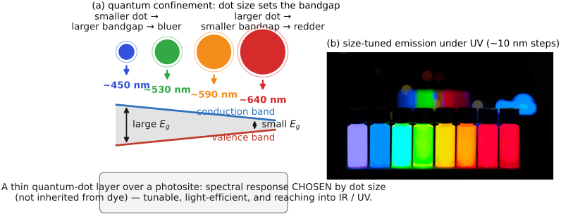
optionalColloidal quantum dots offer size- and material-dependent bandgaps and can form photosensitive layers above a readout circuit. They are useful research and device materials for spectral ranges and integration schemes that differ from silicon. Color-selective layers still need multiple independent measurements, whether distributed spatially or stacked.
A tunable bandgap does not imply an arbitrarily narrow absorption spectrum. Quantum dots can absorb broadly at energies above the band edge, even when their fluorescence is narrow. Nor does replacing a dye with another absorber automatically recover rejected photons. Evaluate absorption, charge extraction, dark current, stability, and cross-channel separation for the proposed architecture.
Multiplexing in depth: stacked photodiodes⧉
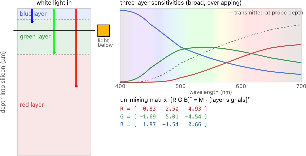
optionalStacked photodiodes use silicon’s wavelength-dependent absorption depth. Short wavelengths are absorbed near the surface; longer wavelengths penetrate farther. The layer signals overlap spectrally, so they require a calibrated color transform rather than being direct red, green, and blue measurements. Foveon designs use this principle; some variants sample deeper layers at lower spatial resolution and still require reconstruction. Noise after color correction depends on the measured layer sensitivities, collection efficiency, and covariance.
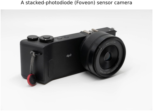
Few production cameras have ever used a Foveon sensor; the Sigma dp series is the best known (Figure 4.6.16), sold on exactly the trade above: unusually crisp, demosaicking-free luminance detail in exchange for noisier color, device-dependent sensitivity and readout limits.
For a simplified collection interval from depths $z_1$ to $z_2$, Beer–Lambert absorption gives the fraction $e^{-\alpha(\lambda)z_1}-e^{-\alpha(\lambda)z_2}$, where $\alpha$ is silicon’s absorption coefficient. This illustrates overlapping depth responses (Figure 4.6.17). Real charge collection also depends on device structure and carrier transport. A broad overlap can make some color distinctions noisy; quantify that through the calibrated transform rather than an invented “unmixing” matrix.
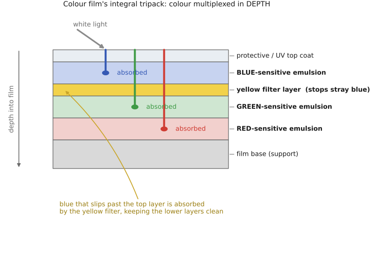
Depth multiplexing is not a silicon invention; color film got there first, chemically. The dominant color-film design, the integral tripack of Kodachrome, Ektachrome, and typical C-41 color negatives, stacks three color-sensitive layer groups, often containing several emulsions, on one base: a blue-sensitive layer on top, then a green-sensitive layer, then a red-sensitive layer, with a thin yellow filter layer just below the top one to stop stray blue (to which all silver halides respond) from leaking into the lower layers. White light enters the top and is caught band-by-band with depth, a similar stacked layout, though spectral sensitization in film differs from absorption-depth separation in silicon, and after development each layer forms its own complementary dye so the stack yields full color at every point with no spatial mosaic (Figure 4.6.18). It is the same trade the Foveon makes and the same one the Autochrome does not: color multiplexed in depth (stacked, full-resolution, no demosaicking) rather than across space (a mosaic that must be interpolated). Silicon's Foveon is the integral tripack rebuilt in a semiconductor, absorption depth standing in for the sensitized layers.
The depth layers are not three bins labeled blue, green, and red. Absorption is probabilistic: at a given wavelength, some photons are absorbed near the surface and others penetrate farther. A shallow collection region therefore receives longer-wavelength contributions as well as short-wavelength ones; deeper regions measure the surviving mixture. The equation above computes the difference between the fractions that reach the top and bottom of an idealized collection interval. This is why three layers need a calibration rather than merely being renamed RGB. When a desired color distinction changes the layer signals only slightly, recovering it can require a large difference of noisy measurements, connecting the sensor architecture to the matrix-noise calculation in Chapter 4.4, RGB color spaces.
Hybrid strategies⧉
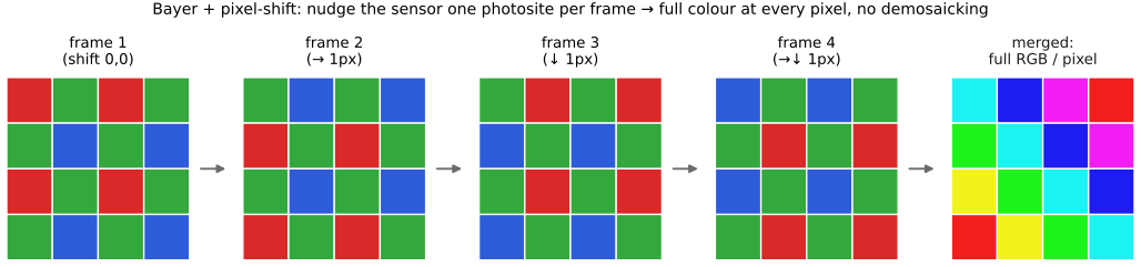
optionalReal cameras often combine strategies, and the most useful hybrid is Bayer plus pixel-shift (Figure 4.6.19). A sensor-shift actuator moves through a specified sequence of one-photosite offsets, so that over four exposures every output location is sampled through a red, a blue, and both green filters in turn; merge the four and you get true R, G, B at every pixel with no demosaicking guesswork (full color resolution and additional samples for noise reduction) at the cost of needing a static scene on a tripod. (It is the spatial Bayer trick borrowing the temporal axis to fill its own holes.) Subpixel offsets can support super-resolution if the optics retain the detail and registration is accurate. Motion and occlusion require detection or fallback processing; more frames also mean more capture time. Video pipelines hybridise the other way, leaning on motion across frames; astrophotography filter wheels are temporal multiplexing with cooled sensors.
Beyond trichromatic capture: full spectrum and multispectral⧉
optionalMultispectral instruments acquire more than three bands; hyperspectral systems sample many closely spaced bands. Filter wheels, scanned spectrometers, filter mosaics, and snapshot spectral encodings trade spectral detail against spatial sampling, time, and noise. A spectral cube is still a finite set of measurements with a calibrated spectral response, not an exact continuous spectrum.
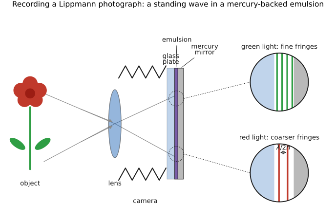
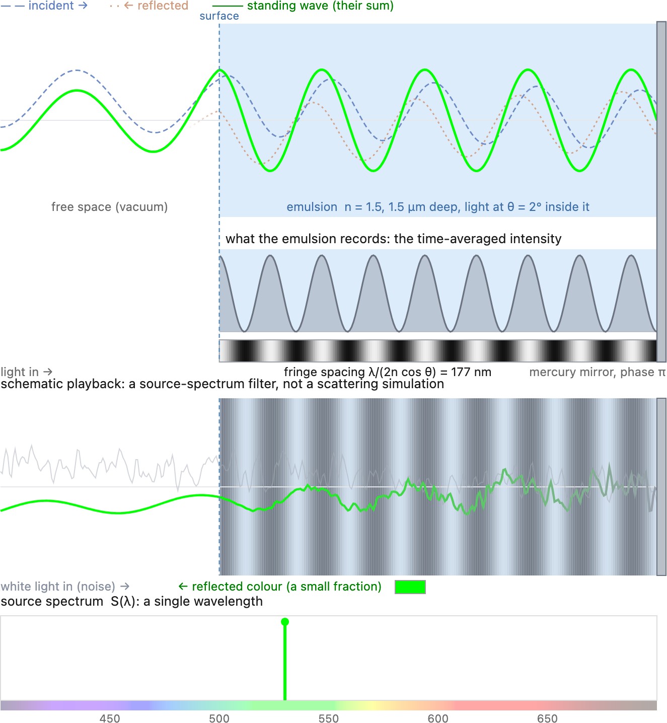
Lippmann photography records spectral information through interference along the depth of an emulsion Lippmann 1891 Lippmann color photography (Alternative Photography) Bjelkhagen, "Lippmann photography". Incident light and its reflection from a backing mirror form depth-dependent intensity fringes. For vacuum wavelength $\lambda$, refractive index $n$, and internal angle $\theta$, adjacent intensity maxima are separated by
After development, the layered structure selectively reflects wavelengths under suitable viewing illumination. Finite thickness limits spectral resolution; the mirror’s phase response, emulsion response, processing shrinkage, and viewing angle affect reproduction. It preserves more spectral information than an RGB photograph, but not a perfect, unlimited record of the original spectrum. Modern recovery methods model these distortions Baechler et al. 2021.
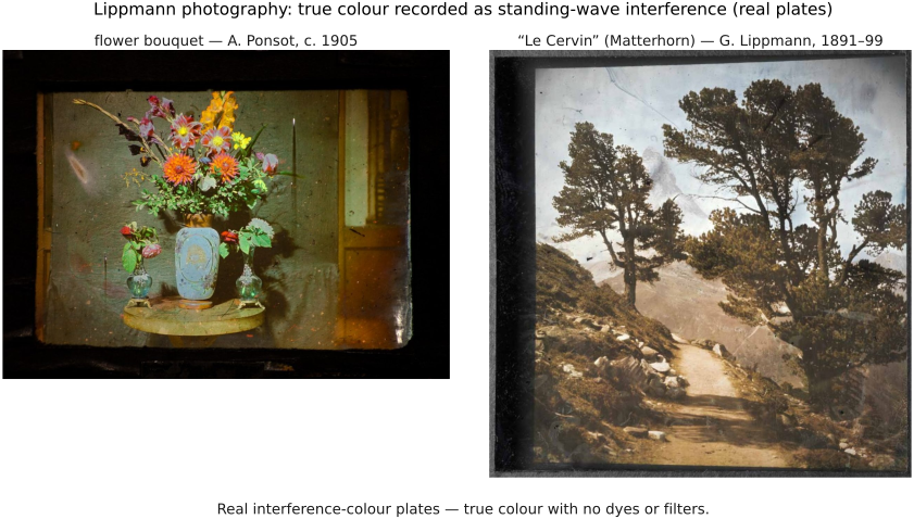
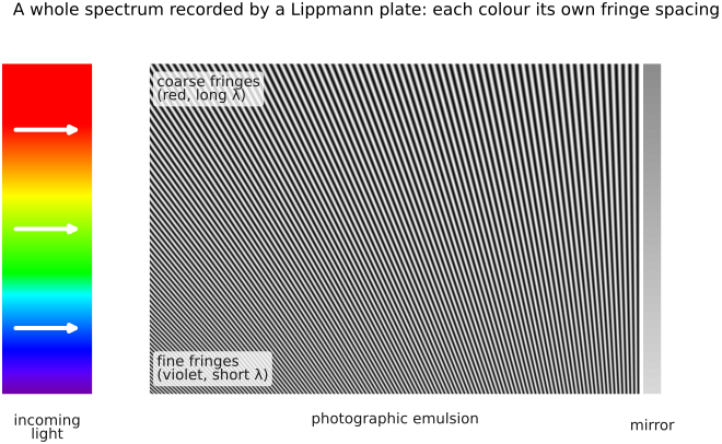
Gabriel Lippmann (1845–1921) received the 1908 Nobel Prize in Physics for interference color photography, the only Nobel awarded for a color-photography process. He was a physicist's physicist: his capillary electrometer was used to record the first human electrocardiogram, he predicted the converse piezoelectric effect that the Curies then confirmed, and he proposed integral photography, an ancestor of light-field imaging. Long exposures and restrictive viewing conditions limited the color process’s practical adoption, but its spectral recording remains an instructive alternative to trichromatic capture.
For a monochromatic exposure, the incident and reflected waves establish a repeated intensity pattern through the depth of the emulsion. Development records that pattern as a layered optical structure. When white light later illuminates it, reflections from successive layers reinforce one another near the recorded wavelength under the appropriate viewing geometry. A more complicated incident spectrum leaves a more complicated depth pattern. The layer spacing carries spectral information even though the emulsion is not divided into conventional red, green, and blue channels. Lippmann's method is therefore a useful counterexample to the assumption that a color photograph must store three numbers: it records another kind of optical measurement, whose reconstruction still has finite bandwidth and physical imperfections.
Spectral sensitivity: matching the eye, catching photons, and white balance⧉
optionalWith photon spectral exposure $q(\lambda)$ and effective channel detection probability $\eta_i(\lambda)$, the expected signal electrons are
The response includes filters, optics, and quantum efficiency under the stated convention. Sampled implementation needs wavelength-bin weights. Shot noise is determined by detected electrons, while read noise is added by the readout; the full model is in Chapter 2.8, Noise, signal-to-noise ratio and dynamic range. A broad response alone is not a color measurement: distinct response shapes supply the information that separates spectra.
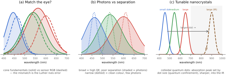
The exact shape of a color sensor's three spectral-sensitivity curves (the $r(\lambda)$ of the red, green, and blue channels, built earlier by the color-filter array on the photosites of Chapter 2.7, Sensors: photosites, CCD vs CMOS) is one of the camera's most constrained choices, because it is pulled in three directions at once that cannot all be satisfied.
- Fidelity to human vision. For a camera to record the color a human would see, its three curves should be a fixed linear combination of the eye's cone fundamentals (equivalently, of the CIE color-matching functions), the Luther–Ives condition. A sensor that met it could be mapped to human color by a single $3\times3$ matrix with no error. Practical camera sensitivities generally only approximate it, because silicon-plus-dye curves are simply the wrong shape, and the penalty is a metameric error no color matrix can remove: two spectra that look identical to the eye read as different RGB, and two that look different can read the same. The color-correction matrix in Chapter 8.10, Auto-exposure and auto white balance is a least-squares compromise: right on average, wrong on the hard cases (saturated reds, narrow-band LEDs, foliage).
- Quantum efficiency and noise. Broad transmission bands can increase total photon collection; this is distinct from quantum efficiency at a specified wavelength: the wider each filter, the more photons reach the well and the higher the SNR. Strong overlap can make color separation poorly conditioned, because separating similar channel responses can require large signed coefficients that amplify measurement noise (compare the distinct physiological opponent processing in Chapter 3.2, Perceptual color and trichromatic vision). Narrow, well-separated filters give clean color but throw photons away and read noisier. The green-doubled Bayer is one point on this curve: spend photons and resolution where the eye cares most (luminance), economize on chroma.
- White balance across illuminants. Because each channel integrates illuminant × reflectance × sensitivity, changing the light changes the raw RGB of a fixed object. Undoing that, white balance often approximates the change with per-channel gains. Matching cone sensitivities does not make this diagonal relighting model exact; a response set that matches human colorimetry well need not be the best basis for diagonal adaptation. Good spectral design makes white balance more reliable across illuminants (→ Chapter 8.10, Auto-exposure and auto white balance).
These three pull against each other: the curves that best match the eye are broad and overlapping (bad for separation), the curves that separate color cleanly are narrow (bad for QE and for matching the eye), and keeping white balance stable across odd illuminants wants yet another shape. Every color sensor is a negotiated settlement among them (Figure 4.6.24).
File formats and compression⧉
RAW files: before the cooking⧉
optionalRaw storage retains data from an earlier stage of the camera pipeline, leaving more reconstruction and rendering choices to the developer. The file may contain a CFA mosaic, demosaicked channels, or partly processed measurements. Raw capture offers latitude, but does not guarantee unmodified or losslessly stored sensor data.
To obtain scene-linear working values, decode the stored representation, apply any linearization table, subtract calibrated black levels, and use the metadata-defined scale. A linear DNG can already contain reconstructed channels. Check processing tags and profiles rather than assuming the extension establishes the numerical domain.
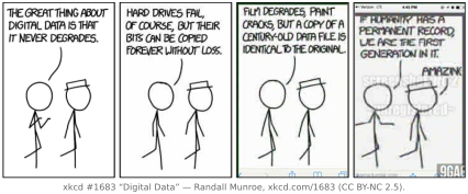
Here is the subtlety, stated plainly: "RAW" is not always purely raw. The name suggests an untouched sensor dump, but in practice most cameras pre-cook the data to some degree: subtracting the sensor's black level, correcting defective and hot pixels, sometimes applying lens-shading or vignetting correction or even mild denoising. Some "RAW" formats are themselves lossy-compressed or non-linearly encoded to save space. So RAW is best thought of as a spectrum of how cooked the data is, from a near-literal readout to something already partly processed, not a single guarantee of pristineness.
There is also a practical headache: RAW is largely proprietary. Nearly every manufacturer ships its own format and extension: Canon's (CR3 files), Nikon's (NEF files), Sony's (ARW files), and so on, each subtly different. That creates software and archival problems, since a format only one company supports may not be readable in thirty years. Adobe's Digital Negative (DNG) format is an open, documented, standardized RAW container meant to fix exactly this (its specification Adobe DNG specification is the reference here); many photographers convert their proprietary RAWs to DNG for safekeeping, and some cameras shoot DNG directly.
You will not parse a proprietary RAW format yourself; a library decodes the mosaic and metadata for you. The classic is dcraw, a single heroic C file that reverse-engineered dozens of formats; its maintained successor is LibRaw (C++), with a friendly Python wrapper, rawpy:
import rawpy
with rawpy.imread("photo.dng") as raw:
    bayer = raw.raw_image.copy()  # retain samples after closing raw
    pattern = raw.raw_pattern
    pattern = None if pattern is None else pattern.copy()
    rgb   = raw.postprocess()      # or let LibRaw develop it to RGB
Beyond these, open-source developers darktable and RawTherapee, Adobe's DNG Converter and DNG software development kit (SDK), and exiftool for metadata round out the toolkit; commercial Lightroom and Capture One are the mainstream developing apps.
Demosaicking and joint methods⧉
A Bayer sensor measures one color at each photosite. A mosaic of red, green and blue filters sits over the pixels, with green on half of them and red and blue on a quarter each, so each pixel records a single filtered value (Chapter 4.6, Sensing color: multiplexing strategies, Figure 15.0.1). Demosaicking reconstructs the two missing values at every pixel.
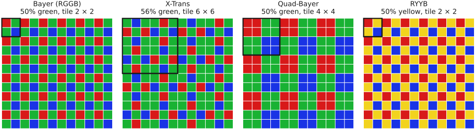
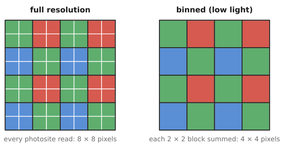
Bayer's is the most common mosaic, not the only one. Fujifilm's X-Trans repeats a 6 × 6 tile with more green than Bayer and at least one pixel of every color in every row and column (Figure 15.0.1). Its less regular layout breaks up the periodic structure that turns fine patterns into color moiré on a Bayer sensor, which lets the cameras that use it leave out an optical low-pass filter, and it needs a demosaicker of its own. Quad-Bayer, common in phone sensors with many small pixels, puts four adjacent pixels under each color filter, a Bayer pattern of 2 × 2 blocks. In low light the sensor combines each block into one larger, less noisy pixel; in good light it reads every pixel and remosaics them into a full-resolution Bayer image (Figure 15.0.2); and the four pixels of a block can be given different exposures to extend dynamic range. Nona-Bayer layouts, Samsung's Nonacell for example, push the same idea to 3 × 3 blocks: a 108-megapixel sensor that bins to 12 megapixels in low light. Other arrays, such as RYYB and RGBW, trade color accuracy for light. Chapter 15.5, Alternative color filter arrays treats these layouts, and Chapter 15.12, Hardware alternatives to the mosaic the sensors that avoid a mosaic altogether.
Demosaicking is one of the fundamentally ill-posed problems of computational photography. We need three numbers per pixel and we have measured one. Many full-color images agree exactly with the same mosaic, and they differ where it matters most, at fine texture and edges, where a wrong choice shows up on fences and fabric as false color, zippering or a maze pattern. Our only hope is to use what we know about natural images, the prior of Chapter 7.1, Imaging as Bayesian inference with probabilistic priors: for example, their color channels share edges, and color varies more slowly than brightness.
This also makes demosaicking hard to measure. On the vast majority of pixels, flat regions, gentle gradients and ordinary edges, almost any reasonable method is nearly exact. The mistakes are rare, but when they happen they are catastrophic and very visible: zippering along an edge, false color on a fence, moiré on fabric, a maze in fine texture. Averaged over a whole image, a few thousand badly wrong pixels among millions barely move a statistic such as mean squared error or PSNR, so two methods can score almost the same while one of them has artifacts that ruin the picture. Demosaickers are therefore judged on the hard cases themselves: error maps, the worst few percent of pixels, and test sets built from the patterns that fail, which is also how the learned methods of Chapter 15.6, Learned demosaicking are trained.
Demosaicking is one of several areas of computational photography, with denoising and super-resolution, where traditional techniques use these regularities implicitly, through the careful design of smart algorithms rather than an explicit model. Interpolating along an edge rather than across it assumes that edges are continuous; interpolating color differences rather than colors assumes that the channels share structure. The field is now changing, from designing algorithms that embody the regularities to learning them from data with deep networks, which can capture regularities no hand-designed rule states. Where each approach runs is set by computation. A camera's image signal processor demosaics every preview and video frame at full resolution in a few milliseconds, so it still runs hand-designed methods of the kind described in Chapter 15.1, Basic traditional demosaicking and Chapter 15.2, Advanced traditional demosaicking. Learned demosaicking has shipped mainly in desktop raw converters, which can spend seconds on one photograph. Phones sit in between: a still photograph gets up to a second or so of processing after the shutter, enough to run networks at full resolution, though manufacturers do not say whether those networks replace the demosaicker, and some phone pipelines avoid single-frame demosaicking by merging a burst of raw frames directly onto a full-color grid.
The part follows that arc. Classical methods rest on two ideas: interpolate along an edge rather than across it, and interpolate a quantity that varies less than the channels themselves, such as the difference between two channels or the residual left after predicting one channel from another Kiku et al. 2013 (residual interpolation). Both assume the channels share structure, which colored edges, clipping and chromatic aberration can violate (Chapter 15.1, Basic traditional demosaicking, Chapter 15.2, Advanced traditional demosaicking). Chapter 15.3, Mosaics and aliasing looks at the mosaics in the Fourier domain, where false color and moiré are aliasing, and at the optical filters that try to prevent it. Chapter 15.4, Optimizing and searching classical demosaickers keeps the hand-made structure and lets data set its constants or search for its structure, Chapter 15.6, Learned demosaicking replaces the rule with a trained one, and Chapter 15.11, Synthetic data, unprocessing, and raw reconstruction asks where the training pairs come from. Demosaicking also interacts with noise: interpolation turns independent sensor errors into correlated color errors, and a denoiser that ignores the mosaic mixes unlike measurements, so Chapter 15.8, Joint demosaicking and denoising and Chapter 15.9, Joint methods and the end-to-end pipeline estimate them together, which helps without automatically beating a well-designed sequence. Chapter 15.10, Quad-Bayer and Nona-Bayer processing covers the grouped layouts of phone sensors, where the industry's remosaicking detour meets learned direct reconstruction. The remaining chapters cover alternative arrays, hardware that avoids the mosaic, and neighboring raw-stage corrections. Throughout, keep the raw measurements and their metadata, the mosaic layout, units, noise and clipping, available to whatever reconstructs the image.
Basic traditional demosaicking⧉
This chapter covers the hand-designed reconstructions, the ones that encode their assumptions about images in the algorithm itself. They start from the layout of the Bayer tile Bayer 1976: the two green-filtered photosites of each 2×2 block sit on one diagonal, red and blue on the other (Figure 15.0.1, at the start of Part 15, Demosaicking and joint methods). Each filter has a broad spectral response, so a photosite records a camera-color component, not a wavelength.
Green gets the extra samples because camera green correlates strongly with brightness, where the eye wants the most detail. It is not colorimetric luminance, though; Chapter 15.3, Mosaics and aliasing makes the split between a combined brightness signal and color explicit.
The crux of the whole problem is that the three colors are measured in different places. Red sits on one sparse grid, blue on another shifted by (1,1) pixel diagonally, green on a denser checkerboard, and no two of them coincide. When the scene has a sharp edge, the three channels cross it at slightly different pixels, and such misregistration is the source of most demosaicking artifacts: zippering, false color and color moiré all come from it, while noise amplification and aliasing already present in the samples have other causes.
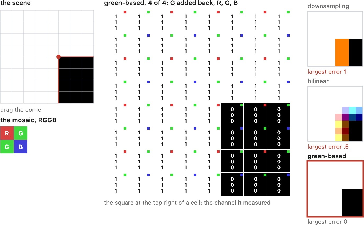
We will illustrate demosaicking with a scene composed of one dark corner on a light background (Figure 15.1.1). It starts from the mosaic itself.
A raw file may contain a CFA mosaic, linear RGB, or partially processed data. Decode its packing and any linearization table, subtract the calibrated black level, and read the CFA pattern and active-area origin. Do not infer these from the extension. Chapter 8.11, File formats and compression discusses storage and metadata.
Test a synthetic constant field first, including unequal constants such as $(0.2,0.4,0.7)$: a correct reconstruction returns each channel's own constant, including at the borders. A real neutral target need not give equal raw channel values before white balance. Then use an achromatic rectangle and a colored edge, and test all four Bayer phases. Those cases expose indexing errors, zippering and failures of the cross-channel assumption.
Keep in mind where demosaicking sits in the pipeline. Raw values are linear in light, and demosaicking works on them in that form; the color-difference methods below depend on it. Its output is therefore still linear camera RGB, not a picture ready for a screen. Before display, it still needs the color matrix to a standard RGB space, usually a tone curve that gives the camera its look (the beauty-curve chapter), and the gamma encoding the display system expects (Chapter 4.3, Encoding: linear, gamma or log). Shown directly, a linear demosaicked image looks dark and flat.
Downsampling and bilinear interpolation, and how they fail⧉
Two simple reconstructions come first, and their failure illustrates the demosaicking challenge.
The simplest is not to interpolate at all. Make each 2 × 2 tile one pixel, taking its red, the mean of its two greens and its blue. Every output value is a measurement, the two greens are averaged, which lowers their noise, and the operation costs almost nothing, which is why raw decoders such as dcraw offer it as a half-size mode and fast previews often use something like it. The first price is resolution: the image has half as many pixels in each direction, so detail that the sensor recorded is thrown away. And downsampling unfortunately does not remove the underlying problem: The red, green and blue of a tile were still measured at different positions, so a tile that an edge cuts in two combines red from one side with blue from the other and gets a color the scene does not have (Figure 15.1.1, stage downsample).
The same happens on real pictures and on test charts, where the comparison with the scene is side by side (Figure 15.1.2, stage downsample).
Bilinear interpolation keeps the full resolution instead. It treats the three color channels as three independent, sparsely sampled images and interpolates each one. For a red pixel missing green, average the four green neighbors; for a green pixel missing red, average the two horizontal or two vertical red neighbors, and so on.
It is a useful inexpensive baseline. It reproduces some smooth signals well, but its errors on fine structure illustrate the consequences of sparse color sampling.
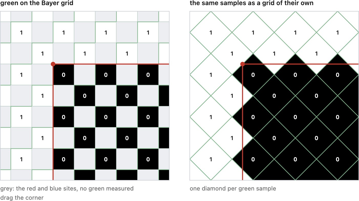
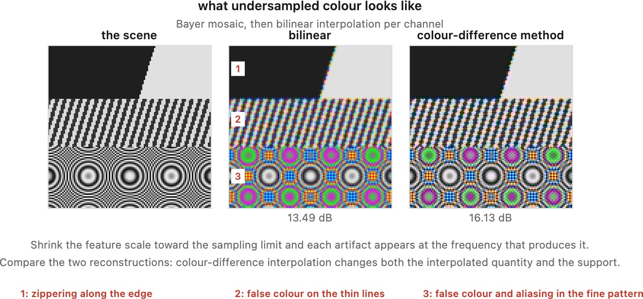
Zippering is an alternating light-dark pattern along a sharp horizontal or vertical edge. It comes from averaging across the edge: at one pixel the four neighbors are two on each side, at the next they are three and one, so the interpolated value alternates. The name comes from what it looks like. The zipper is a form of aliasing (Figure 15.1.3). Green's samples lie on a checkerboard, and a checkerboard is itself a regular square grid, of spacing $\sqrt2$ pixels and turned by 45 degrees, a pattern called a quincunx. To that turned grid, a horizontal or vertical edge of the scene is a diagonal line, and a regular grid samples a diagonal line as a staircase, the same jaggies a diagonal shows on a screen. Bilinear interpolation reconstructs the staircase rather than the edge, and the steps of the staircase are the zipper's teeth.
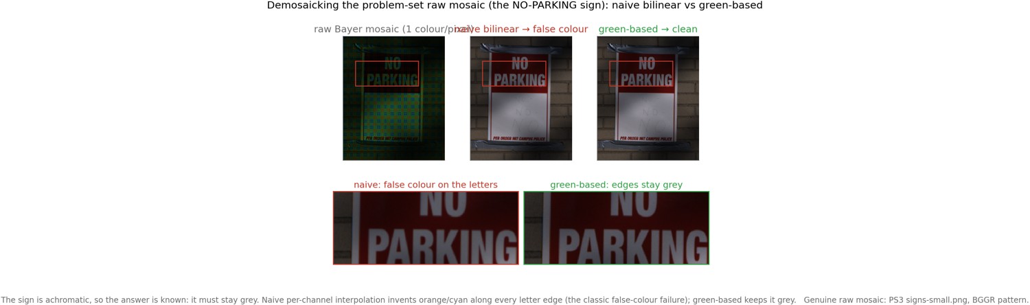
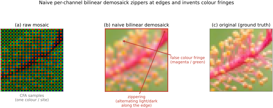
False color is a colored fringe on fine detail that is gray in the scene. It happens because the three channels are sampled at different positions, so a thin structure lands on a red pixel and misses the blue ones, and the interpolation reports a color the scene did not have.
Maze-like patterns often involve unstable direction choices in adaptive methods. They should not be attributed to a bilinear filter changing its interpolation direction.
These artifacts can involve aliasing, cross-channel disagreement and interpolation rules. Looking at their appearance helps diagnosis, but does not uniquely identify the algorithm or cause.
Concretely, for green, whose measured samples lie on a checkerboard, the four nearest measured neighbors sit above, below, left and right:
Red and blue are sparser, so the geometry varies: at some empty sites the nearest red samples are the four diagonal ones, at others the two horizontal or two vertical. The principle is the same, and it is a small tent kernel applied per channel.
The zipper is worth doing with numbers once. Take a vertical black-and-white edge, value 0 against value 1, and look only at green. At a missing green site just on the white side, three green neighbors can be white and one black, giving 0.75 instead of 1, while the measured green site beside it stays at 1. The reconstruction therefore alternates between measured and interpolated positions, which is exactly the run of teeth. On the black side the same averaging lifts missing values above zero.
The corner showed the same numbers along a whole edge (Figure 15.1.1, stages bilinear-green and bilinear-rb).
Interpolate along the edge, not across it⧉
The first classical idea: decide, per pixel, which direction is safe to interpolate in.
For a missing green value, compute a horizontal and a vertical gradient from the available samples, and interpolate along whichever direction varies less. The test goes back to Robert Hibbard's Kodak patent Hibbard 1995 (Kodak patent): compare the differences between the green neighbors horizontally and vertically, and interpolate horizontally, vertically or from all four neighbors depending on which gradient falls below a threshold. Hamilton and Adams's method (Hamilton & Adams 1997) does this with a test that uses both the green neighbors and the same-color neighbors two pixels away, which is what lets a red pixel estimate the second derivative of the red channel and use it to correct the green interpolation.
The second term is the correction that makes this work, and it is the second classical idea arriving early: it uses the red channel's curvature at the center to sharpen the green estimate, on the assumption that the channels share their structure.
Variants differ in how the direction is chosen. Variable number of gradients (Chang, Cheung & Pan 1999 (VNG)) computes gradients in eight directions and averages the ones below a threshold, which handles corners and diagonals better than a two-way choice. Adaptive homogeneity-directed interpolation (Hirakawa & Parks 2005 (AHD)) reconstructs the image both ways, converts both to a perceptual color space, and keeps the version that is locally more homogeneous in color, which is a defensible criterion because the eye tolerates luminance detail and not chrominance noise.
The plain two-direction form of the same idea is worth seeing before the correction term arrives:
Interpolate along whichever axis its two neighbors look most alike, on the bet that the other axis crosses an edge. The bet rests on the world being piecewise smooth: mostly flat regions separated by a relatively small number of strong, roughly one-dimensional edges. Get those right and the cases the eye notices are handled. A tie can take the four-neighbor average rather than preferring an axis, and continuous directional weights avoid abrupt switches. Fine periodic texture can make both directional differences misleading, and noise can flip the choice.
On the corner, the rule picks the right pair at every cell (Figure 15.1.1, stage edge-green).
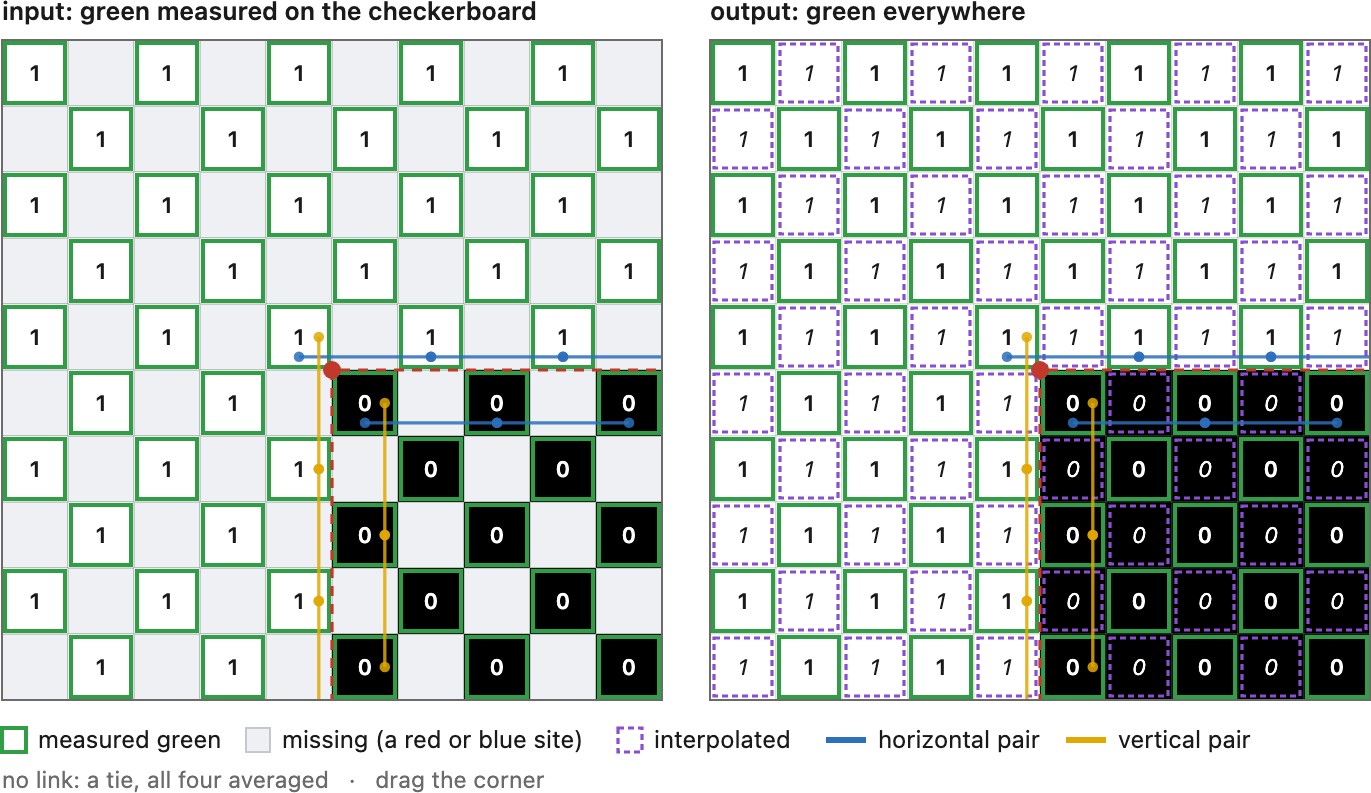
Edge-directed demosaicking is a first, very concrete instance of a theme that returns throughout the book: adapt the operation to the local structure of the image rather than applying the same fixed filter everywhere. Here the structure is an edge and the adaptation is choosing the interpolation direction; later, in edge-preserving filtering and denoising, the same instinct (use the similarity between pixels to decide how much they should influence each other) becomes the bilateral filter and the idea of affinity. Whenever a fixed linear filter blurs across something it should have respected, the cure is to look at the data first.
# edge-directed green interpolation, the Hamilton-Adams test
dH = abs(G[x-1,y] - G[x+1,y]) + abs(2*R[x,y] - R[x-2,y] - R[x+2,y])
dV = abs(G[x,y-1] - G[x,y+1]) + abs(2*R[x,y] - R[x,y-2] - R[x,y+2])
if   dH < dV: G_est = (G[x-1,y]+G[x+1,y])/2 + (2*R[x,y]-R[x-2,y]-R[x+2,y])/4
elif dV < dH: G_est = (G[x,y-1]+G[x,y+1])/2 + (2*R[x,y]-R[x,y-2]-R[x,y+2])/4
else:         G_est = average_of_both
This pseudocode is for a red center; exchange red and blue at a blue center. Copy measured green samples in noiseless interpolation and use a CFA-aware boundary extension that preserves color parity. Malvar–He–Cutler provides a useful fixed linear alternative with cross-channel Laplacian corrections (Malvar et al. 2004); it differs from selecting a direction per pixel.
Edge-directed green is the simplest case of a more general idea, steered reconstruction (Chapter 6.5, Resampling and upsampling). Reconstructing a sampled image means choosing, at each output pixel, weights for the nearby samples: a reconstruction kernel. A fixed kernel, like bilinear's, uses the same weights everywhere, so it blurs across edges and aliases along them. A steered kernel is shaped by the local image, long along an edge and narrow across it, so it averages where the signal is smooth and keeps the change sharp (Figure 6.5.19). The two-direction green rule is its coarsest version: two candidate kernels, one horizontal and one vertical, and a gradient test to choose between them. The variants above refine the choice. VNG considers eight directions, AHD compares whole reconstructions, and the Hamilton–Adams correction adds information from the other channels to the kernel it chose.
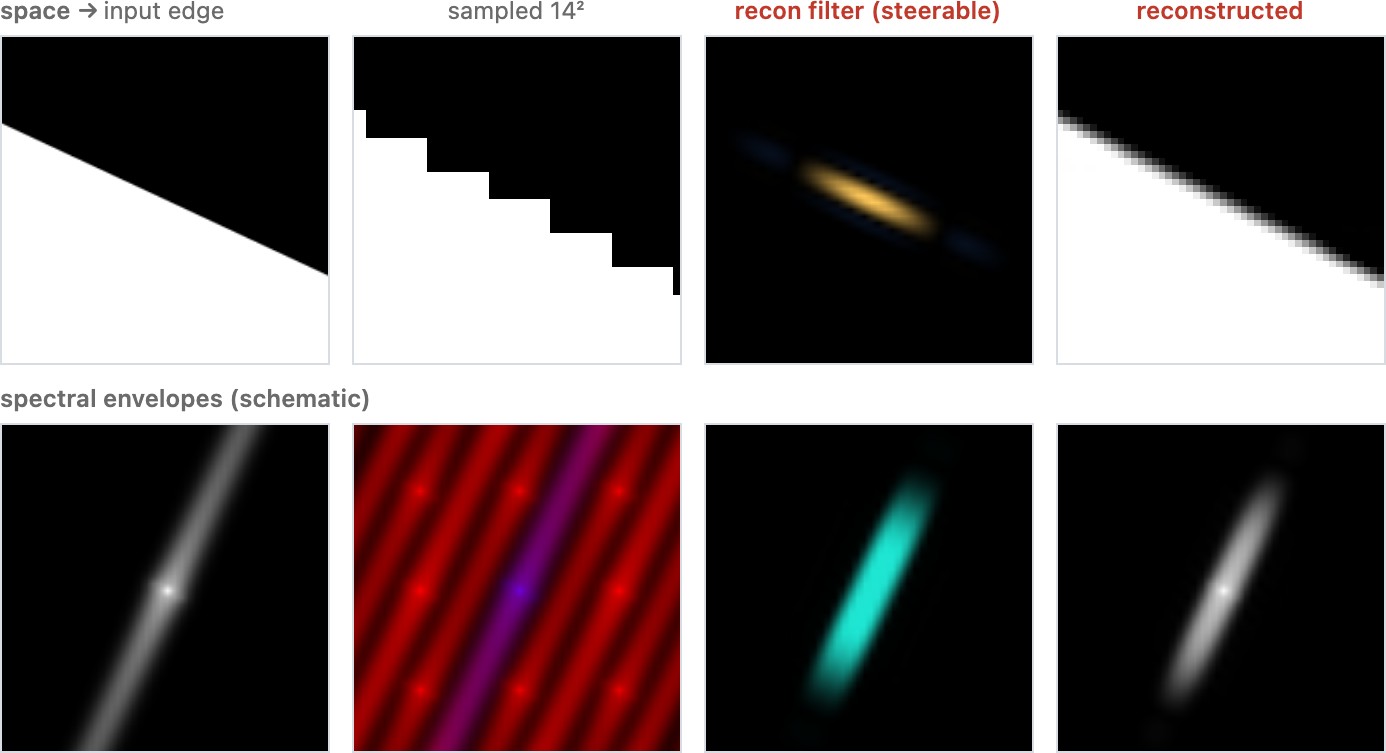
Working out the local reconstruction weights from the local pattern is the key idea of traditional demosaicking, and it reaches beyond it. Kernel regression makes the steering continuous, estimating an orientation and an elongation at every pixel from the local gradients (Chapter 10.7, Locally adaptive regression kernel (LARK)). RAISR learns a bank of filters and picks one per pixel by hashing the local gradient pattern (Chapter 14.4, Single-image super-resolution: classical methods); applied to a mosaic, the same scheme would amount to a learned gradient test. None of these methods writes down an image prior, yet each encodes one in the rule that chooses the weights: that the image is smooth along some direction at every pixel. Chapter 15.6, Learned demosaicking replaces the hand-written rule with one fitted to data.
Interpolate differences, not channels⧉
The second classical idea does more work than the first and is less often stated plainly.
Color differences can vary more slowly than individual channels, especially near neutral structure. They are not invariant to shading: if $R=rI$ and $G=gI$ for a common shading signal $I$, then $G-R=(g-r)I$, which varies unless $g=r$. The ratio $R/G=r/g$ is constant under this simplified model, but becomes unstable near zero green and changes at material or illumination boundaries.
So interpolate the difference. Estimate green everywhere first, since it is sampled twice as densely, then form $G - R$ at the red pixels, interpolate that smooth quantity, and recover red as $\hat R = \hat G - \widehat{(G-R)}$. The hard, high-frequency part of the problem is solved once, in the channel with the best sampling, and the other two channels inherit it.
On the corner, the differences are formed at the red and blue sites (Figure 15.1.1, stage differences).
Green-first reconstruction is common, but other joint and frequency-domain methods do not follow that ordering. Difference interpolation fails when the assumed shared structure is weak: strongly colored edges, channel clipping and chromatic displacement are important cases.
As a recipe, in four steps:
- Reconstruct green everywhere, using the edge-directed method above, since green has the densest sampling.
- Form the difference $R - G$ at every pixel where red was measured, and $B - G$ at every measured blue pixel, which is possible now that green exists everywhere.
- Interpolate the difference with plain linear interpolation and no edge logic, because the difference is usually the smoother quantity. Sharp color boundaries remain the failure case.
- Add green back: $R = (R-G) + G$, and likewise for blue.
An achromatic edge has zero true color differences, so this keeps it gray, but only if the reconstructed green is also accurate at the measured red and blue sites. Green errors leave residual false color even on that simple target.
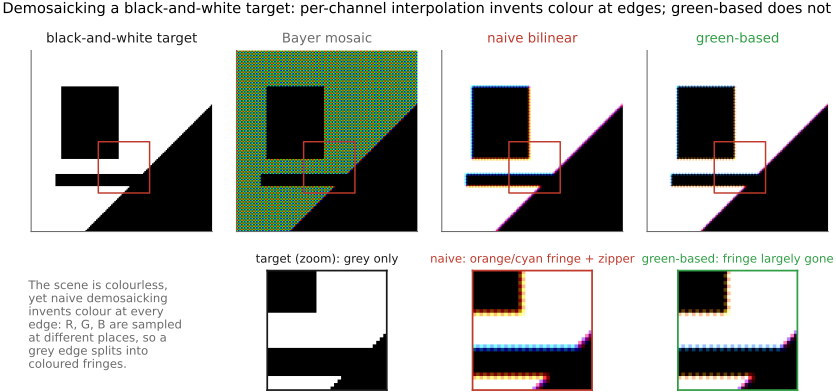
Channel differences are often smoother than luminance-like structure, which makes guided reconstruction useful. Preserve that distinction as an image model rather than a law: fine color texture and saturated boundaries can break it.
We interpolated the difference $R - G$. A natural alternative is the ratio $R / G$, which encodes the assumption that hue (the proportion of red to green) is locally constant (the "constant-hue" model), and which can behave better than the difference when brightness varies a lot within a region. Ratios bring their own headache: $G$ can be near zero in the shadows, and dividing by a small noisy number is asking for trouble. In practice the difference is simpler and more robust, the ratio can be sharper on saturated colors, and real pipelines mix or switch between them. The shared idea, interpolate color (a relationship between channels), not the raw channels, is what matters.
Even green-based, edge-directed demosaicking is not perfect. Fine, high-frequency color texture, a tiled roof, a striped shirt, a picket fence, breaks the smooth-color assumption and produces the residual false color often called maze or labyrinth artifacts, because at those scales the channels really are doing different things. That is where the modern methods earn their keep.
Where the maze comes from shows up best on a small patch of fine texture (Figure 15.1.9). At a pixel where the horizontal and vertical tests come out nearly equal, a little noise decides which one wins, so neighboring pixels choose differently, and the pattern of choices is the labyrinth.
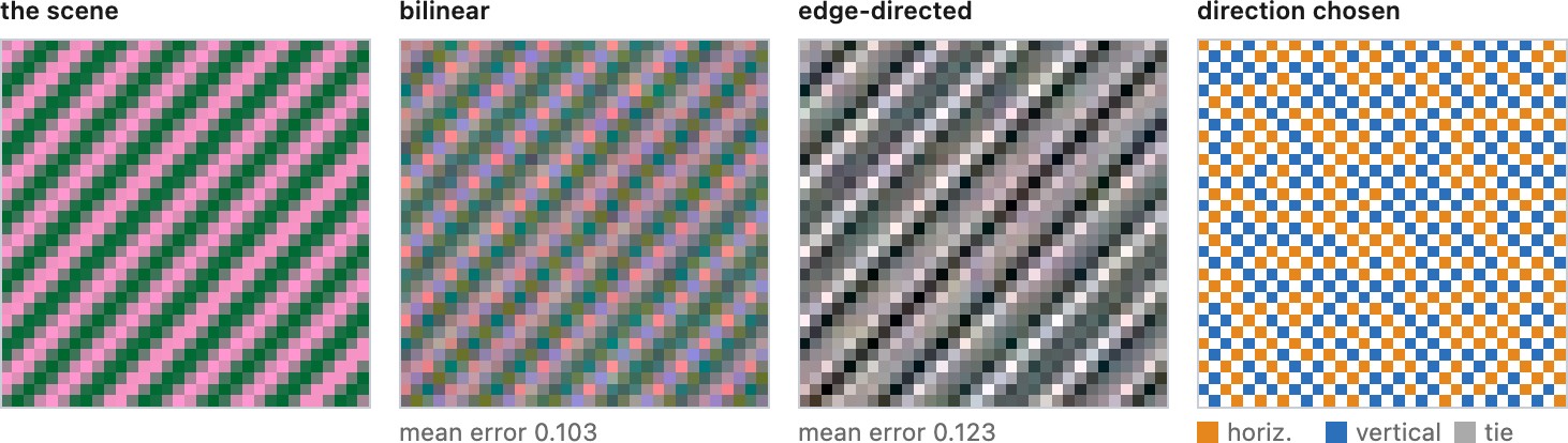
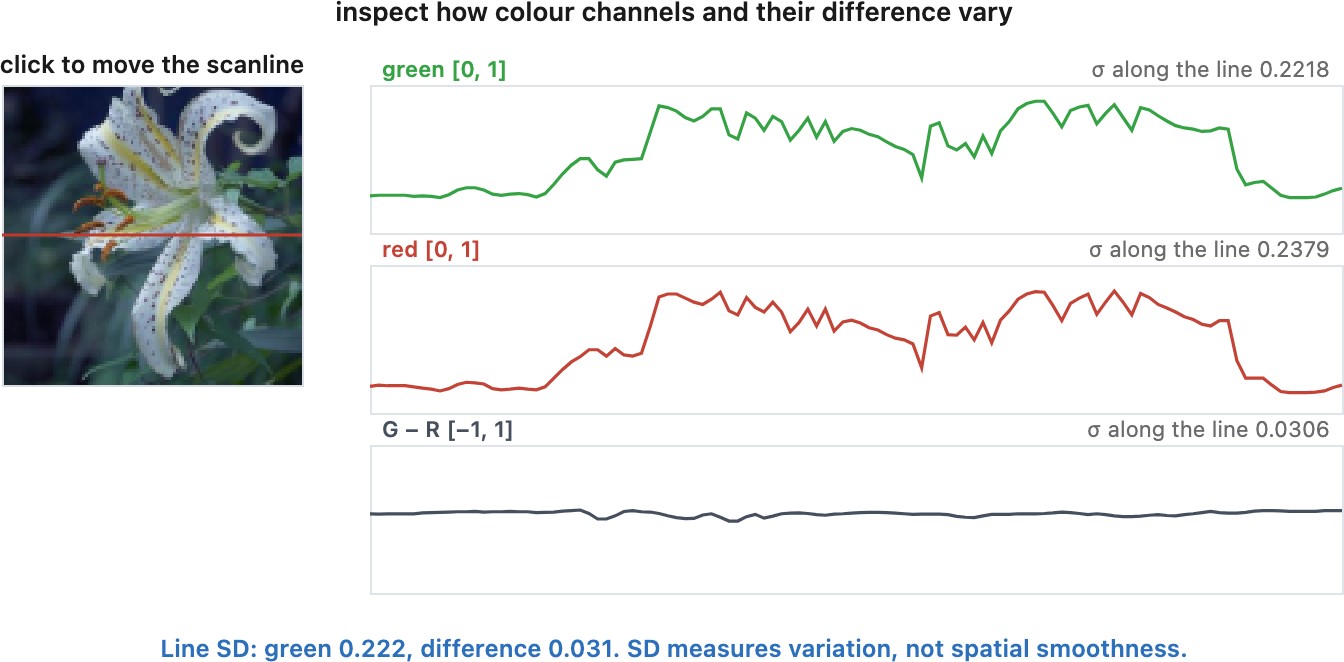
A red flower against green leaves is a useful counterexample to the shared-edge assumption: the boundary can have very different contrast in red and green. A clipped specular highlight breaks the linear relationship for another reason, because one channel stops increasing while another still responds. Lateral chromatic aberration breaks it geometrically by placing the same boundary at different coordinates. These cases need different remedies even when their demosaicked outputs all show colored fringes.
Demosaicking and other aspects of imaging⧉
optionalDemosaicking is one part of an imaging system. The optics and the sensor decide what the mosaic records, and the stages of the camera pipeline around it (Part 8, Basic image processing and ISP) decide what it is handed and what happens to its output. Each method in this chapter and in Chapter 15.2, Advanced traditional demosaicking assumes something about its input, and these other parts decide whether the assumption holds.
The anti-aliasing filter. Many cameras place an optical low-pass filter in front of the sensor. It blurs the image slightly before sampling, so that less fine detail aliases into color moiré, the failure no demosaicker can fully undo because the mosaic cannot tell it from real color. Many recent cameras have weakened or dropped it and leave moiré to the demosaicker. Chapter 15.3, Mosaics and aliasing explains what the filter can and cannot remove, and why it has been disappearing.
Grouped layouts: Quad and Nona. Phone sensors that group same-color photosites in 2 × 2 (Quad-Bayer) or 3 × 3 (Nona-Bayer) blocks change what a demosaicker receives. In low light the sensor bins each block and hands over an ordinary Bayer mosaic at a quarter or a ninth of the pixel count, and the methods of this chapter apply unchanged. At full resolution the same color is repeated over neighboring sites, so red, for example, is missing from larger regions than in a Bayer mosaic, and the nearest red sample can be three photosites away. A Bayer demosaicker applied directly to that layout uses the wrong colors at most sites; the usual route is to remosaic the grouped layout into an estimated Bayer mosaic first, which is itself an interpolation, then demosaick, or to demosaic the grouped layout directly (Chapter 15.10, Quad-Bayer and Nona-Bayer processing).
Color routers. A nano-prism or metasurface color router keeps the Bayer layout but steers each band of light toward the photosite that measures it instead of absorbing it (Chapter 4.6, Sensing color: multiplexing strategies). Each photosite then collects light from a wider area than its own, which acts as a mild anti-aliasing filter (Chapter 15.3, Mosaics and aliasing), and part of each band lands on neighbors of the wrong color, which broadens and mixes the channels' spectral responses. The demosaicking algorithms still apply, but the color correction that follows has to undo more mixing.
Black level. The sensor adds an offset to every sample, and it has to be subtracted first. Color differences and ratios are meaningful only on values proportional to light: with the offset left in, a gray edge no longer has a constant $R-G$ across it, and the ratio model of the "difference or ratio?" sidebar is wrong everywhere.
Defects and lens shading. A hot or dead photosite is one wrong sample, and interpolation copies it into its neighbors' missing colors, so a single bad value becomes a colored speck several pixels across; repair it on the mosaic. Lens shading darkens the corners by a different amount in each channel, which demosaicking would read as color. Both are covered in Chapter 15.7, Neighboring problems in the raw stage.
White balance. The color-difference methods work best when a neutral surface has equal values in all three channels, because then the difference across a gray edge is zero on both sides and interpolating it is exact. Raw values under most lights are far from equal for a neutral, so many pipelines apply the white-balance gains to the mosaic before demosaicking (Chapter 8.10, Auto-exposure and auto white balance). The gains then scale clipped samples too: a highlight that clipped in green is no longer at a common ceiling once red and blue are multiplied, which is where pink highlights come from, so saturated samples need to be marked before the gains are applied.
Chromatic aberration. Lateral chromatic aberration shifts the color channels relative to one another toward the edges of the frame. The cross-channel assumption then fails exactly at edges, where it is needed, and a demosaicker reads the misregistration as a colored edge. Correcting it before or during demosaicking avoids fringes that are much harder to remove afterward (Chapter 22.2, Aberrations correction).
Noise. Interpolation mixes neighboring samples, so independent sensor noise becomes spatially correlated color noise, which is harder for a denoiser to recognize. Noise also flips the edge-direction decisions of this chapter. Denoising the mosaic first, or demosaicking and denoising together, avoids both (Chapter 15.8, Joint demosaicking and denoising).
After demosaicking. The color matrix, tone curve and sharpening all act on the reconstructed image, and sharpening in particular amplifies zippering and maze patterns along with real detail (Chapter 8.8, Sharpening). A demosaicker that leaves small artifacts can look acceptable until the rest of the pipeline has run, so judge it on the finished rendering as well as on its direct output.
The practical rule is to know which of these steps have been applied to the data a demosaicker receives, in what units, and to tell the algorithm.
And all of it should happen on linear values. Black-level subtraction, defect repair, lens-shading and white-balance gains, and demosaicking itself operate on numbers proportional to light, and the image becomes nonlinear only afterward, when the tone curve and the gamma encoding prepare it for display. The reasons are the ones this chapter keeps meeting. Interpolation averages, and an average of gamma-encoded values is not the encoding of the average light, so a demosaicker run on encoded values darkens fine detail and shifts colors at edges (Chapter 6.5, Resampling and upsampling). Color differences and ratios describe the scene only when the values are proportional to light. And the noise model that joint methods rely on is simple only in linear units, before a curve stretches the shadows and compresses the highlights.
Advanced traditional demosaicking⧉
optionalThe methods below, published between the late 1980s and the mid-2000s, combine the two ideas of Chapter 15.1, Basic traditional demosaicking, edge direction and color differences, in different proportions, and hand-designed methods of this family are still what most cameras and phones run in their image signal processors, where a demosaicker must run on every preview and video frame, fast, small and predictable. Learned demosaicking has shipped mainly in desktop raw converters, such as Adobe's Enhance Details and DxO's DeepPRIME, which also denoises (Chapter 15.6, Learned demosaicking). Some phone pipelines avoid single-frame demosaicking altogether by merging a burst of raw frames directly onto a full-color grid (Chapter 14.2, Multi-frame super-resolution). Figure 15.2.1 runs ten of them side by side on the same mosaic, including the residual interpolation and ARI of this chapter, so each method's assumption can be seen where it fails.
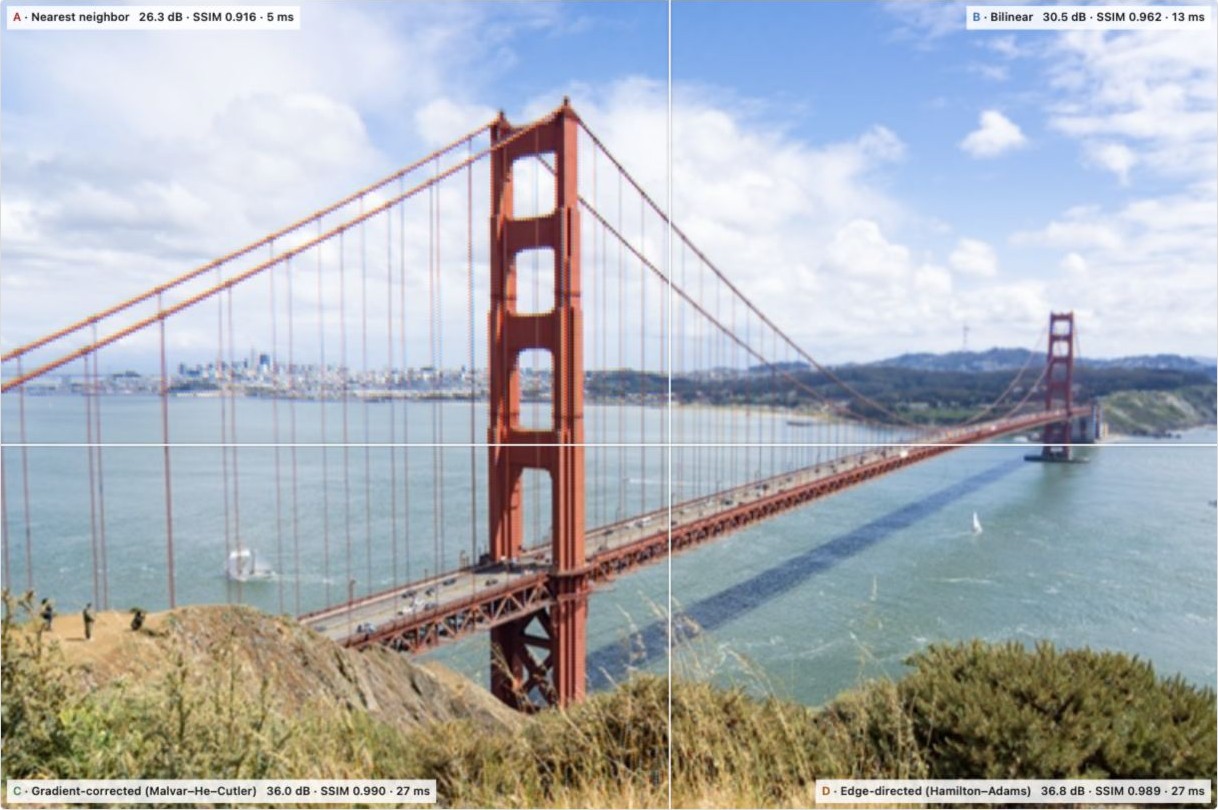
Nearest neighbor copies each missing value from a nearby sample of the right color, with no arithmetic. The name is loose, because most sites have several equally near samples of a given color: a red site has four green neighbors at the same distance, and four blue ones on the diagonals. An implementation breaks the tie with a fixed rule, usually by working tile by tile. In the lab's version, every pixel of a 2 × 2 tile takes that tile's one red and one blue, a green site keeps its own green, and the other two sites take the same one of the tile's greens. That makes it a close relative of the downsampling of Downsampling and bilinear interpolation, and how they fail: downsampling turns each tile into one pixel, and nearest neighbor is almost that same small image blown back up to full size by copying each value into the four pixels of its tile. The only differences are that the measured greens stay where they were and nothing is averaged. Nearest neighbor therefore keeps the pixel count but adds almost no detail over downsampling, and it keeps downsampling's flaw: each color is attributed to a place up to a pixel away from where it was measured, so every edge becomes a colored staircase, the strongest zipper of any method here. It costs nothing, which is why it survives in live previews and thumbnails. Bilinear interpolation (Downsampling and bilinear interpolation, and how they fail) averages instead of copying and fixes the misregistration in smooth regions, not at edges.
Figure 15.2.2 works through every method of this section on a small mosaic, one step per stage, starting with nearest neighbor.
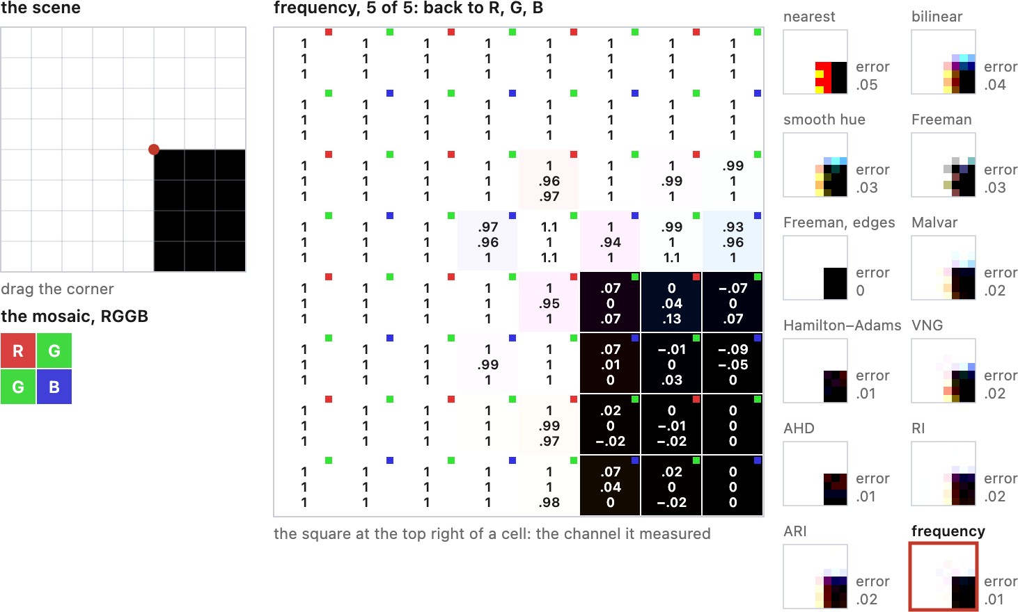
Smooth hue transition Cok 1987 (smooth hue transition), one of the first methods to use one channel to reconstruct another, interpolates green first and then interpolates hue rather than red and blue: the ratio $R/G$ at the red sites, spread to its neighbors and multiplied back by green. It assumes that hue changes slowly across an object even where brightness does not. The choice of hue coordinate matters, and the lab lets you switch it: a ratio becomes unstable where green is near zero, a difference $R-G$ does not, and a log ratio sits in between. The difference form is the recipe of Interpolate differences, not channels.
Its three steps are the smooth-hue stages of Figure 15.2.2.
Freeman's method Freeman 1988 (median demosaicking) demosaicks with bilinear interpolation, then cleans up the hue: it applies a 3 × 3 median to the difference channels $R-G$ and $B-G$ and adds green back. Within an object the color difference is nearly constant, so a false-color pixel is an isolated outlier in a flat channel, which is exactly what a median removes. A 5 × 5 median often does a better job, because false color on fine texture tends to come in clusters wider than a 3 × 3 window can outvote, though a larger median also starts to carry color across object boundaries. The median does nothing for zippering in the green channel, so although the method is described on top of bilinear, it is mostly used as a clean-up step on top of a better demosaicker. Figure 15.2.1 offers both bases: on bilinear, the median removes most of the fringes and leaves the zippering; on the chapter's edge-based demosaicking, the green is already good and the median only has the remaining false color to remove. The same pass survives as the final clean-up of many later methods, AHD among them. (Freeman's patent differs in its details: it describes two colors alternating along a line, interpolates each linearly, and applies a one-dimensional median to their difference, five pixels wide in its example, with each pixel keeping its own measured value. The two-dimensional Bayer version above is the one usually implemented.)
Figure 15.2.2 shows the three steps on the grid.
Gradient-corrected linear interpolation Malvar et al. 2004, by Malvar, He and Cutler, keeps a fixed linear filter but adds the Laplacian of the channel measured at the center pixel, scaled by a gain, to the bilinear estimate of each missing channel. A red pixel's curvature, for example, corrects the green estimated there, on the assumption that the channels vary together. The result is a set of fixed 5 × 5 filters with no decisions, so it is fast, easy to run on a GPU, and free of the unstable direction choices that make mazes; it is, for example, what MATLAB's demosaic function implements. Because it does not adapt, it still blurs across edges where an adaptive method would not.
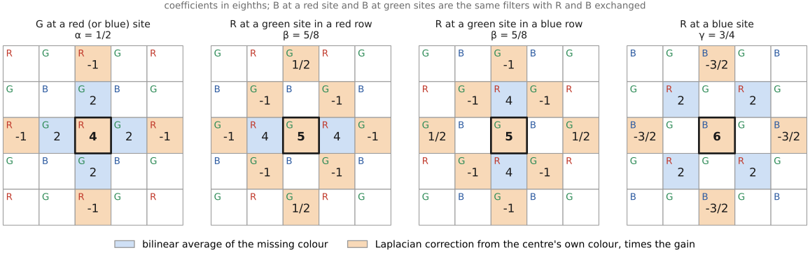
The same correction, pixel by pixel, is in Figure 15.2.2.
Hamilton–Adams Hamilton & Adams 1997, met in Interpolate along the edge, not across it, combines both ideas of the basic chapter, and it does so in three passes over the mosaic, each using the channels already filled in.
- Green at the red and blue sites. Measure a horizontal and a vertical activity at the site, each the sum of a green gradient across the site and the second difference of the center color along the same line. Interpolate green along the less active direction, as the average of its two green neighbors plus a quarter of the center color's second difference, and use all four neighbors when the two activities are equal. This is the pseudocode of Interpolate along the edge, not across it.
- Red and blue at the green sites. Now that green exists everywhere, a missing red at a green site is the average of its two red neighbors, horizontal or vertical depending on the row, corrected by half of green's second difference along that line. It is color-difference interpolation in disguise: the result equals the site's green plus the average of the two neighbors' $R-G$, up to the correction.
- Red at the blue sites, and blue at the red sites. The four nearest samples of the missing color sit on the diagonals, so the method chooses between the two diagonals with the same kind of test, a gradient of the missing color along the diagonal plus green's second difference along it, and interpolates along the calmer one with the same half-weight correction.
# Hamilton-Adams, steps 2 and 3 (step 1, green, is in the edge-directed section)
# step 2: red at a green site in a red row (blue rows: use the vertical pair)
R[x,y] = (R[x-1,y] + R[x+1,y])/2 + (2*G[x,y] - G[x-1,y] - G[x+1,y])/2

# step 3: red at a blue site, choosing a diagonal
dN = abs(R[x-1,y-1] - R[x+1,y+1]) + abs(2*G[x,y] - G[x-1,y-1] - G[x+1,y+1])   # NW-SE
dP = abs(R[x+1,y-1] - R[x-1,y+1]) + abs(2*G[x,y] - G[x+1,y-1] - G[x-1,y+1])   # NE-SW
if   dN < dP: R[x,y] = (R[x-1,y-1] + R[x+1,y+1])/2 + (2*G[x,y] - G[x-1,y-1] - G[x+1,y+1])/2
elif dP < dN: R[x,y] = (R[x+1,y-1] + R[x-1,y+1])/2 + (2*G[x,y] - G[x+1,y-1] - G[x-1,y+1])/2
else:         R[x,y] = (R[x-1,y-1] + R[x+1,y+1] + R[x+1,y-1] + R[x-1,y+1])/4 \
                       + (4*G[x,y] - G[x-1,y-1] - G[x+1,y+1] - G[x+1,y-1] - G[x-1,y+1])/4
# blue at a red site: the same, with R and B exchanged
The corrections are what separate it from bilinear. Each one assumes that the missing channel curves the same way as the channel that was measured or already reconstructed at the site, so a sharp edge in green is copied into red and blue at the same place instead of being smeared into a fringe. The direction tests are what separate it from Malvar–He–Cutler, which applies the same kind of correction everywhere, in every direction. Hamilton–Adams costs a small, fixed amount of work per pixel, and its green step is the starting point of many later methods, including the residual interpolation of the next chapter; its failures are those of any two-way choice: diagonal texture, and fine patterns where both directions look equally active.
Figure 15.2.2 runs the three passes on the grid; the grating near 45 degrees shows the failure.
Variable number of gradients Chang, Cheung & Pan 1999 (VNG), VNG, by Chang, Cheung and Pan, replaces the two-way choice with a vote among eight directions, and lets the image decide how many of them to trust. At each pixel it works in the 5 × 5 neighborhood around the site, in four steps.
- Eight gradients. For each compass direction, north, northeast, east and so on, sum the absolute differences between pairs of same-color samples that lie along that direction on that side of the pixel. Pairing same-color samples keeps the gradient free of the differences between channels. A direction that points into a smooth region gets a small gradient; one that crosses an edge gets a large one.
- A threshold. From the smallest gradient $g_{\min}$ and the largest $g_{\max}$, set $T = 1.5\,g_{\min} + 0.5\,(g_{\max}-g_{\min})$. The threshold is relative: it asks which directions are nearly as smooth as the smoothest one here, not which are below a fixed number, so the same rule works in shadows and highlights.
- A vote. Keep every direction whose gradient is below $T$. For each kept direction, average the samples of each color that lie on that side of the pixel, and sum these averages over the kept directions, one sum per color.
- A color difference. Estimate each missing color from the center sample and the difference of the sums: at a red site, for instance, $\hat G = R + (S_G - S_R)/n$, where $S_G$ and $S_R$ are the sums for green and red over the $n$ kept directions. This is the color-difference idea of Interpolate differences, not channels, averaged over the directions the vote allowed.
# VNG at one pixel, in outline (per-site sample weights omitted)
g = {d: gradient(d) for d in [N, NE, E, SE, S, SW, W, NW]}       # same-color pairs along d
T = 1.5*min(g.values()) + 0.5*(max(g.values()) - min(g.values()))
keep = [d for d in g if g[d] <= T]
S = {c: sum(average_on_side(c, d) for d in keep) for c in [R, G, B]}  # one sum per color
for c in missing_colors:
    value[c] = center_value + (S[c] - S[center_color]) / len(keep)
The number of directions that pass is what gives the method its name and its behavior. In a flat region all eight pass and it averages widely, which suppresses noise; along a straight edge only the two directions parallel to it pass, and it averages along the edge like Hamilton–Adams; at a corner or a line end it can keep three or four, which a two-way choice cannot express (Figure 15.2.4). The cost is about eight gradients per pixel over a 5 × 5 window, several times Hamilton–Adams, and the relative threshold can pass too many directions in fine, low-contrast texture, where everything looks equally smooth. VNG was long one of the modes of the dcraw raw decoder.
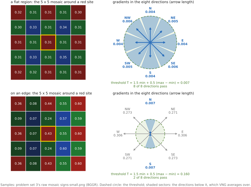
Figure 15.2.2 runs VNG on every pixel of the grid.
Two further refinements are common. Iteration: once green and the color differences are in, re-estimate the differences against the interpolated green and repeat. Alternating projections Gunturk, Altunbasak & Mersereau 2002 (alternating projections) formalize this as projecting in turn onto two sets, the images that agree with the measured samples and the images whose red and blue have the same fine detail as green. And directional estimation with explicit noise models: Zhang and Wu's directional linear minimum mean-square-error method Zhang & Wu 2005 (DLMMSE) fuses the horizontal and vertical estimates with weights set by how noisy each one is, rather than choosing one.
Across the eight panes, three things change from method to method. The assumption about images: smooth channels, smooth hue, correlated channels, or edges along one of a few directions. The decision made at each pixel: none for bilinear and Malvar–He–Cutler, a direction for Hamilton–Adams, VNG and AHD (#Adaptive homogeneity-directed demosaicking (AHD), next). And the cost, from nothing for nearest neighbor to two full reconstructions and a color-space conversion for AHD. The residual-interpolation methods (#Residual interpolation and ARI) take the next step by replacing the color difference with the residual of a guided fit.
For reproducible comparisons, state the implementation and demosaicking mode. LibRaw and dcraw expose several algorithms, but their defaults are not interchangeable with the Malvar–He–Cutler method. Compare against a strong classical baseline such as adaptive residual interpolation Monno et al. 2015 (adaptive residual interpolation) as well as a simple linear method.
The sections that follow take up three families that go further: AHD, which builds whole reconstructions in two directions and keeps the more homogeneous one; residual interpolation and ARI, which interpolate what a guided prediction leaves over; and frequency-domain demultiplexing, which treats the mosaic as a modulated signal. The chapter ends with the situations that defeat all of them.
Adaptive homogeneity-directed demosaicking (AHD)⧉
optionalIf you want to implement one classical demosaicker that is simple and works well, this is probably your best bet, followed by Freeman's median of the color differences (earlier in this chapter) to remove the false color that remains. Every method so far decides the interpolation direction before interpolating, from gradients in the mosaic. Adaptive homogeneity-directed demosaicking Hirakawa & Parks 2005 (AHD), by Hirakawa and Parks, decides afterward. It reconstructs the whole image twice, once interpolating only horizontally and once only vertically, and at each pixel keeps whichever reconstruction looks more plausible there. The criterion is the key idea: interpolating in the wrong direction averages across an edge and creates colors that exist on neither side of it, so the wrong candidate is less homogeneous, locally, than the right one.
- Two candidates. Build a full image with every interpolation along rows: green with a Hamilton–Adams-style correction, then red and blue by interpolating color differences. Build a second with every interpolation along columns.
- A perceptual space. Convert both candidates to CIELAB, so that lightness and color can be compared separately and a distance means roughly what a viewer would notice (Chapter 4.5, Advanced color: opponents, perceptually-uniform, and preferred).
- Homogeneity. For each pixel of each candidate, count the neighbors in a small window that are close to it in both lightness and color, within thresholds $\varepsilon_L$ and $\varepsilon_C$. The thresholds are set at every pixel from the differences to its nearest neighbors along each candidate's own direction, so the test adapts to local contrast rather than using one number for shadows and highlights.
- The choice. Sum each candidate's counts over a 3 × 3 window and keep, at each pixel, the candidate with the larger sum; average the two on a tie.
- Clean-up. Finish with a few passes of a median over the color differences $R-G$ and $B-G$, Freeman's clean-up.
# AHD, in outline
Ih, Iv = demosaic_along_rows(mosaic), demosaic_along_columns(mosaic)
Lh, Lv = to_cielab(Ih), to_cielab(Iv)
eps_L, eps_C = adaptive_thresholds(Lh, Lv)             # per pixel, from nearest-neighbor differences
Hh = count_close_neighbors(Lh, eps_L, eps_C)           # lightness and color both within threshold
Hv = count_close_neighbors(Lv, eps_L, eps_C)
Hh, Hv = box_sum_3x3(Hh), box_sum_3x3(Hv)
out = where(Hh > Hv, Ih, where(Hv > Hh, Iv, (Ih + Iv) / 2))
out = median_color_differences(out, passes=3)
Figure 15.2.5 shows the homogeneity test at one pixel.
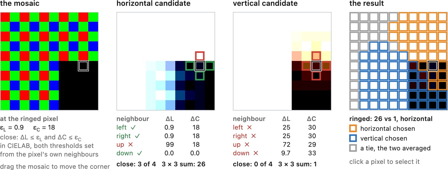
The figure below runs it on a real facade, where the cornice's horizontal lines choose the horizontal candidate and the window columns the vertical one (Figure 15.2.6), and Figure 15.2.2 makes the same choice cell by cell on the chapter's small inputs.
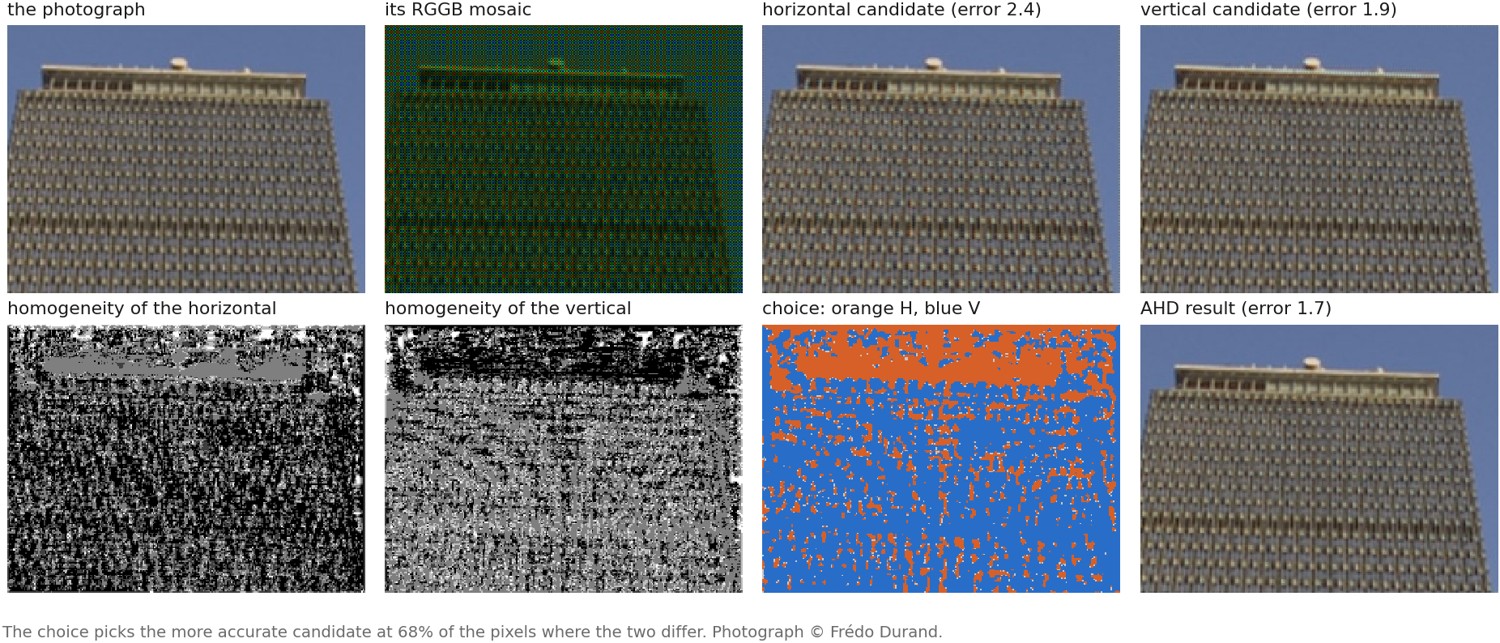
Figure 15.2.2 steps through the same algorithm on the small inputs.
AHD costs two full reconstructions, two color-space conversions and the counting, several times Hamilton–Adams. It was the default of the dcraw raw decoder and of many converters built on it for years, and it is still a strong classical baseline. Its limits are the other methods' limits. It still chooses between two directions, so diagonal texture gives both candidates errors and the choice cannot fix them. In fine texture near the sampling limit both candidates are inhomogeneous and the choice becomes erratic, which is where mazes come from. And noise lowers the homogeneity of both candidates everywhere, so the choice degrades as the noise rises, one reason to denoise first or jointly (Chapter 15.8, Joint demosaicking and denoising).
Residual interpolation and ARI⧉
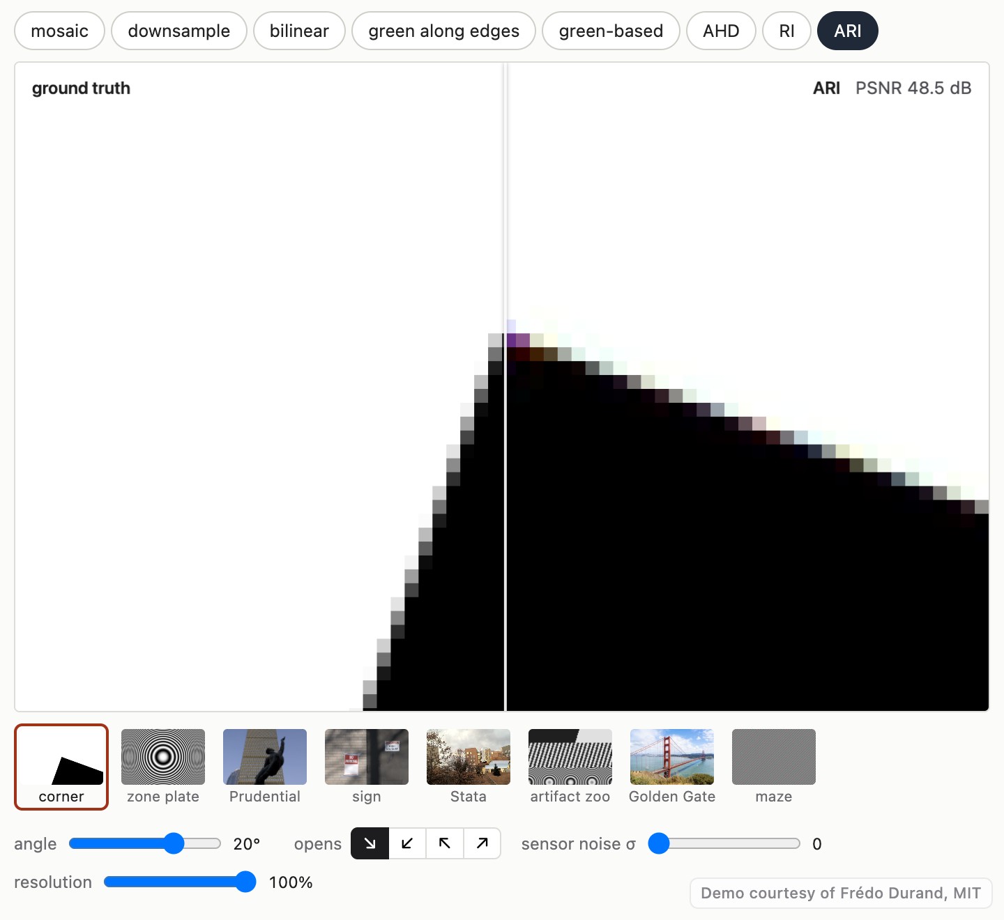
optionalThe best-performing classical demosaickers, and the ones to compare against today, come from the residual-interpolation family, and adaptive residual interpolation (ARI) is its strongest member. It appeared a decade after AHD, outperforms it clearly in published comparisons on the standard test sets, and needs no training. It is also built directly on the guided filter of Chapter 10.6, Guided image filtering, so it is a payoff of that chapter rather than a new tool. It takes more work to implement than AHD, which remains the simpler choice when that matters.
The idea changes what gets interpolated. Every classical method interpolates something, and each step of the classical line chose a flatter quantity. Bilinear interpolates the channel itself and fails at edges. Hamilton–Adams and its successors interpolate the color difference $G-R$, which is smooth wherever the two channels differ by an offset, and fails where that assumption does: at a saturated color boundary, at a specular highlight, wherever the ratio between the channels changes rather than their offset. Residual interpolation Kiku et al. 2013 (residual interpolation), by Kiku, Monno, Tanaka and Okutomi, goes one step further. Rather than hope that some quantity is flat, it constructs one: it fits a local prediction of the sparse channel from the dense one and interpolates only what the prediction gets wrong.
Take red, sampled on a quarter of the pixels, and green, already reconstructed everywhere because it is sampled twice as densely. In a small window, model red as a linear function of green,
with $a$ and $b$ estimated from the red samples that exist in that window. This is a guided filter with green as the guide He, Sun & Tang 2013 (guided filter), restricted to the measured sites. In a window $\Omega$, with $\mathcal R$ the set of sites where red was measured, solve
where $\epsilon>0$ stabilizes the slope. Unmeasured sites must not enter the fit as zeros; a window with no red sample has to grow or fall back to a simpler estimate; and since every pixel lies in many windows, the overlapping predictions are averaged, which is the guided filter's own rule. The tentative estimate $\tilde R$ is a full-resolution red built entirely out of green's structure, and it follows a change of contrast between the channels that a difference cannot. The residual is the part of red that green cannot explain,
and the reconstruction interpolates it, by any simple method, and adds it back:
The prediction carries the shared detail, and the residual corrects its errors where measurements constrain them. When the local model explains the structure the channels share, the residual is smaller and flatter than the color difference, and the same cheap interpolator does much less damage to it. That flatness is an assumption to test, not a property the fit enforces: a small residual at the measured sites does not prove that the residual between them is small or smooth, and a misleading guide, a sharp color boundary or a poorly conditioned fit can transfer the wrong structure into the result.
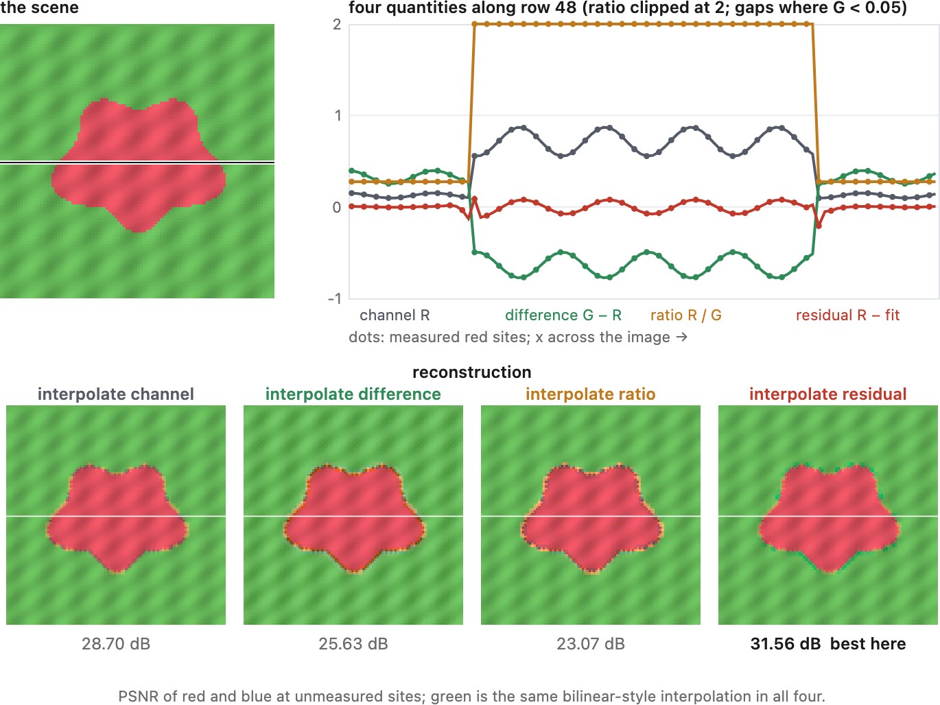
The full algorithm applies the same idea twice, first to green and then to red and blue.
- Green first. Estimate green along rows and along columns separately, each time guiding by the measured red or blue along that line and interpolating the residual along it, then combine the two directional estimates with weights that favor the direction whose color differences vary less locally.
- Tentative red. With the full green as the guide, fit a local linear model $\tilde R = aG + b$ in each window, using only the sites where red was measured, and evaluate it everywhere.
- Residual. At the measured red sites, form $R-\tilde R$.
- Interpolate and add back. Interpolate the residual bilinearly to every site and add it to $\tilde R$. Blue is the same with blue's samples.
On a red flower against green leaves, the residual is close to zero where the color difference is large, and residual interpolation scores 3.3 dB above AHD (Figure 15.2.8).
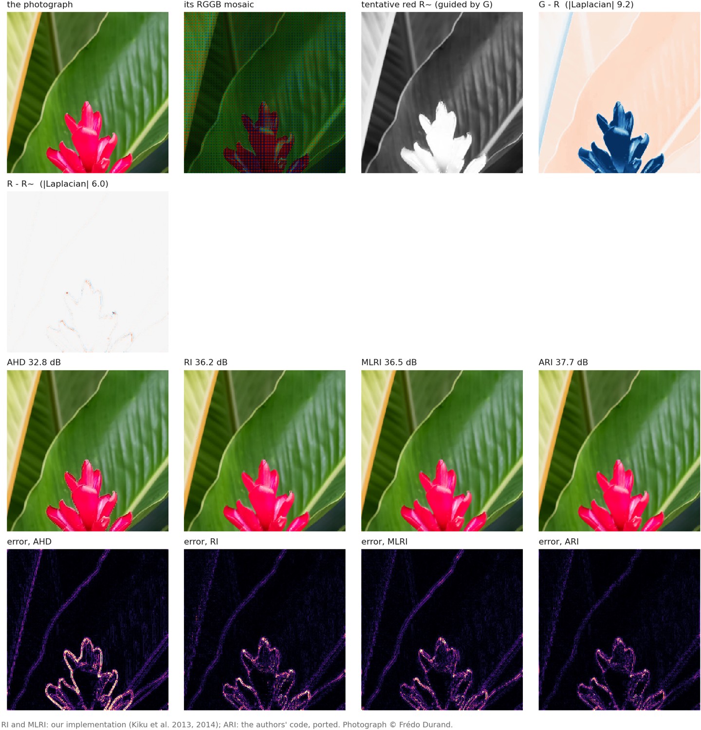
Minimized-Laplacian residual interpolation, MLRI Kiku et al. 2014 (minimized-Laplacian residual interpolation), changes only how $a$ and $b$ are fitted: instead of least squares on the values, it minimizes the Laplacian energy of the residual, which is what the final bilinear interpolation needs to be small. It changes how the regression coefficients are estimated, not which channel serves as the guide. ARI Monno et al. 2015 (adaptive residual interpolation), by Monno, Kiku, Tanaka and Okutomi, iterates both, using each output as the next guide, and at each pixel selects the variant and the number of iterations whose residual is smoothest, judged by the local fit. That is the direction-selection idea of Hamilton–Adams operating one level up: not which direction to interpolate in, but which method to trust here. A later version extends it to multispectral filter arrays Monno et al. 2017 (ARI, multispectral). The authors' reference code has been used widely enough in later work that comparisons against it can be trusted.
# Residual interpolation for red, green already reconstructed (blue is the same)
def residual_interpolation(G, R_mosaic, red_mask, radius, eps):
    a, b = masked_guided_fit(guide=G, target=R_mosaic, mask=red_mask, radius=radius, eps=eps)
    R_tent = box_mean(a, radius) * G + box_mean(b, radius)     # guided filter output
    residual = where(red_mask, R_mosaic - R_tent, 0)
    return R_tent + bilinear_from_samples(residual, red_mask)

# MLRI: the same, with a and b fitted to minimize the Laplacian of the residual
# ARI, in outline: at each pixel keep the (method, iteration) whose residual is smoothest
estimates = []
guide = G
for k in range(K):
    for method in [RI, MLRI]:
        R_k = method(guide, R_mosaic, red_mask)
        estimates.append((R_k, laplacian_energy(R_mosaic - R_k, red_mask)))
    guide = R_k
R = per_pixel_argmin(estimates)          # smoothest residual wins, in a local window
Figure 15.2.2 steps through residual interpolation cell by cell on the chapter's small inputs, from the directional green to ARI's per-pixel choice, and the demosaicking lab at the start of this chapter (Figure 15.2.1) runs the same code on photographs.
The limits are the guided filter's. A local linear model cannot follow channels that are related nonlinearly, at clipping or under strong chromatic aberration, and fitting $a$ and $b$ from a few noisy samples is unstable, so noise should be removed first, accounted for within the fit, or handled by joint reconstruction (Chapter 15.8, Joint demosaicking and denoising).
This family, not bilinear interpolation, is the baseline a learned demosaicker should be measured against. It embodies three separate decisions: predict one channel from a guide, interpolate what the prediction missed, and choose locally between useful variants. A learned model can change any of the three, and a comparison with bilinear alone leaves those established improvements unaccounted for, so it cannot tell which part of a network's gain required learning. Compare actual accuracy, noise assumptions and runtime; no ranking of classical methods, and no fixed advantage in decibels, carries over across datasets and settings. A network can represent similar cross-channel predictions, but it chooses what to interpolate implicitly, which is one reason it is hard to say what it learned: a benchmark gain does not show that it learned this algorithm, and attributing the gain requires controlled experiments rather than an analogy between architectures (Chapter 15.6, Learned demosaicking).
Demosaicking as demultiplexing: frequency-domain methods⧉
optionalOne family of methods treats the mosaic the way a radio engineer treats a signal. As Chapter 15.3, Mosaics and aliasing shows, a Bayer mosaic is exactly a luma component $L$ plus two chroma components modulated onto carriers at the highest frequencies the grid supports: $C_1$ on the horizontal and vertical carriers, $C_2$ on the diagonal one,
Demosaicking is then demultiplexing: isolate each modulated chroma band with a bandpass filter, shift it back to baseband by multiplying by its carrier, and take the luma as what remains. Alleysson, Süsstrunk and Hérault Alleysson, Süsstrunk & Hérault 2005 (frequency-domain demosaicing) arrived at this from the side of human vision, where luma and chroma are carried separately; Dubois Dubois 2005 (frequency-domain demosaicking) made it adaptive. Nowhere else in this chapter is the algorithm itself the frequency argument, rather than a heuristic that happens to be analyzable in frequency terms.
- Diagonal chroma. Filter the mosaic with a bandpass filter centered on the diagonal carrier and multiply by $(-1)^{i+j}$ to bring $C_2$ back to baseband.
- Axial chroma, twice. $C_1$ is carried twice, on the horizontal and on the vertical carrier. Extract it from each with its own bandpass filter and demodulate.
- Choose the cleaner copy. Luma detail leaks into the two copies differently: a vertical texture puts its energy near the horizontal carrier and spoils that copy, while the vertical copy stays clean. Dubois weights the two estimates at each pixel by the local energy of the crosstalk in each, which is the edge-direction idea of this chapter moved into the frequency domain.
- Luma. Remodulate the chroma estimates and subtract them from the mosaic; what remains is $L$.
- Back to RGB. $G=L-C_2$, $R=L+C_2+2C_1$, $B=L+C_2-2C_1$.
# frequency-domain demosaicking (Dubois style), for an RGGB mosaic y
C2  = lowpass(bandpass(y, carrier=(pi, pi)) * alternate(i + j))
C1h = lowpass(bandpass(y, carrier=(pi, 0))  * alternate(i))
C1v = lowpass(bandpass(y, carrier=(0, pi))  * alternate(j))
eh, ev = local_energy(crosstalk_h), local_energy(crosstalk_v)   # luma leaking into each copy
C1  = (ev * C1h + eh * C1v) / (eh + ev)                         # trust the cleaner copy
L   = y - C1 * (alternate(i) + alternate(j)) - C2 * alternate(i + j)
G, R, B = L - C2, L + C2 + 2*C1, L + C2 - 2*C1
Figure 15.2.2 runs the same demultiplexing on the small inputs.
The filters are where the quality lives. Leung, Jeon and Dubois Leung, Jeon & Dubois 2011 (least-squares luma-chroma demultiplexing) design them by least squares on training images rather than by hand, the least-squares luma-chroma demultiplexing that is the version to cite for performance: a small learned element inside an entirely classical structure. The limit is the one Chapter 15.3, Mosaics and aliasing names: where luma and chroma overlap in frequency, as on fine texture near the carriers, no linear filter can separate them, and the leftover luma shows up as false color.
On the upper floors of a tower facade, where the window grid approaches the carriers, choosing the cleaner copy of $C_1$ per pixel removes much of the false color that averaging the two copies leaves, and the method scores above AHD (Figure 15.2.9). The same implementation falls below bilinear interpolation on the flower of Figure 15.2.8, whose saturated edges carry chroma at frequencies the low-pass filters remove.
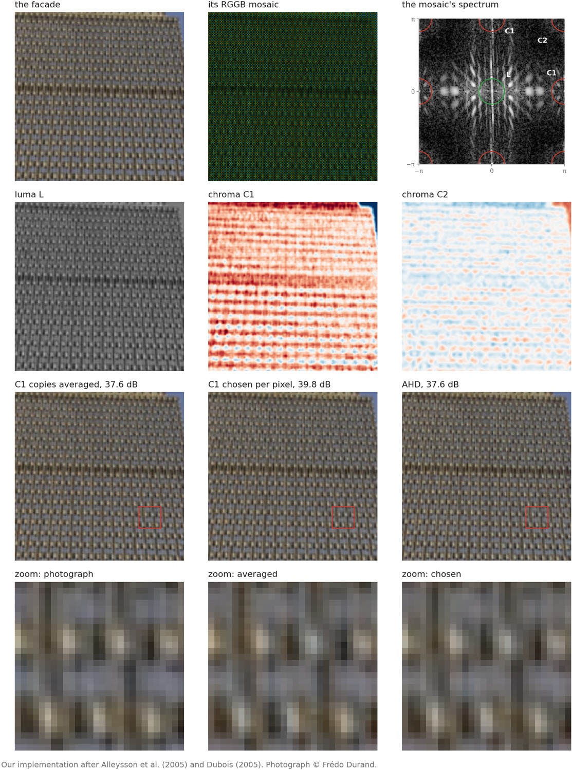
Where the classical methods stop⧉
optionalFour situations defeat this family, and they are worth listing because the learned methods of Chapter 15.6, Learned demosaicking are judged on exactly them.
Diagonal edges can challenge a horizontal/vertical decision. More directions or a broader model can help; failure is not inevitable on every diagonal.
Repetitive texture near the sampling limit can alias into apparently consistent false structure. Wider context helps some cases, but a single mosaic may leave genuine ambiguity.
Clipped samples no longer report the incident signal linearly. Mark them and avoid treating their color differences as ordinary measurements. The amount of recoverable highlight color depends on which channels remain useful.
Noise perturbs gradients and can switch interpolation decisions. The error depends on signal-to-noise ratio, not ISO alone. Chapter 15.8, Joint demosaicking and denoising incorporates this uncertainty in reconstruction.
Mosaics and aliasing⧉
All channels at once: luma and chroma⧉
optionalThe mosaic is one image, not three, and its spectrum is the sum of the three sampled channels. Because the masks add up to one at every pixel, their impulses away from zero cancel for a gray scene: whatever sits at a carrier frequency is a difference between channels. For Bayer, with red at even-even positions and blue at odd-odd positions, the algebra is exact and short:
At even-even positions the expression gives $R$, at mixed parity $G$, and at odd-odd positions $B$, which is a direct implementation check; a different origin for the array changes the signs of the carriers. The luma $L$ is a mixture of camera channels, not CIE luminance. Multiplication by $(-1)^i$ shifts a spectrum by $1/2$ cycle per pixel, so the mosaic is the luma at baseband plus $C_1$ modulated onto the two axis carriers $(1/2, 0)$ and $(0, 1/2)$, plus $C_2$ modulated onto the diagonal carrier $(1/2, 1/2)$ (Alleysson, Süsstrunk & Hérault 2005 (frequency-domain demosaicing); Dubois 2005 (frequency-domain demosaicking)). Given separated components, $G=L-C_2$, $R=L+C_2+2C_1$ and $B=L+C_2-2C_1$.
The luma is sampled at every pixel and keeps the full band of the pixel grid. The chroma is what pays for the mosaic: it is recorded only as copies parked at the highest frequencies the grid supports. This works because natural images have much less chroma detail than luma detail, so the chroma copies are compact and mostly stay clear of the luma band. Chapter 15.2, Advanced traditional demosaicking used this model as an algorithm, filtering the chroma copies out and shifting them back; here it is a way of seeing what goes wrong.
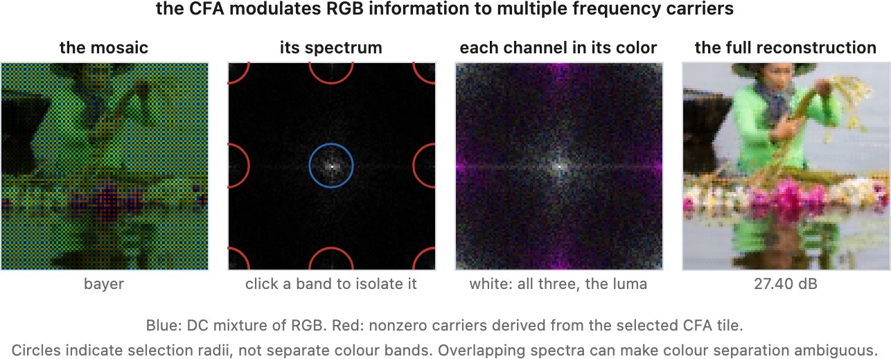
False color and moiré as spectral overlap⧉
optionalAliasing on a mosaic is the luma band reaching a chroma carrier. Fine gray detail near $1/2$ cycle per pixel, a fence, a woven fabric, the fine print on a page, puts luma energy exactly where a demosaicker looks for chroma. The demosaicker cannot tell the two apart and reports a color the scene did not have: false color. A pattern whose frequency is close to a carrier, but not on it, beats against the carrier and produces a slow colored ripple: color moiré. Where the luma band and a chroma copy overlap, the mosaic does not determine which is which, and no reconstruction can separate them without an assumption about the scene. Image context and priors, including learned ones (Chapter 15.6, Learned demosaicking), make better guesses, and extra captures (Chapter 15.12, Hardware alternatives to the mosaic) remove the ambiguity; none of this recovers arbitrary overlapping signals from one mosaic.
Foreshortening makes this common. A fine pattern on a surface that recedes from the camera, a floor, a roof, a striped shirt turned away, grows finer on the sensor with distance, so it sweeps through every frequency on its way to the horizon and passes the carriers at some distance or angle, where the colors appear (Figure 15.3.3).
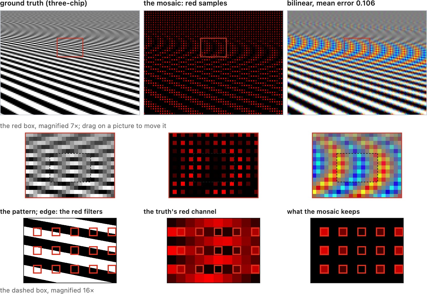
The same picture explains the two greens. Green carries half the luma, so doubling it keeps the luma band wide, while red and blue enter mostly through the chroma, whose narrow band the sparser lattice can hold. This is a statement about natural images and about the eye, which also resolves luma more finely than chroma, and not about green light as such. A sharp colored pattern, red text on a blue sign, violates the assumption and aliases in the chroma itself.
The model is global and images are not. A photograph is smooth in some regions and finely textured in others, so a filter that separates the bands correctly in one place is wrong in another; the adaptive methods of Chapter 15.2, Advanced traditional demosaicking estimate the local structure and change the filter accordingly. The carrier positions describe an array, not the error of a particular demosaicker on a particular image Hirakawa & Wolfe 2008 (spatio-spectral sampling).
Learned demosaicking⧉
optionalFine fabric and thin diagonal structures can defeat local interpolation rules. A learned demosaicker uses a larger training collection to fit how sparse color samples map to full-color detail.
A synthetic training pair is easy to construct by selecting one component per pixel from a full-color image. Producing a representative clean target is harder: a processed photograph may already contain demosaicking, denoising, sharpening and compression artifacts, and its RGB channels need not be camera-linear responses.
Specify the color domain and how the target was prepared before treating remosaicking as a sensor simulation.
Joint demosaicking and denoising⧉
optionalA noisy raw mosaic contains missing color components and uncertain measured samples. Demosaicking and denoising can therefore benefit from a shared estimator. A denoiser that ignores the CFA mixes unlike colors; a demosaicker that ignores noise can make poor direction decisions and spread their errors.
These are failures of particular models and interfaces, not proofs that either sequential order must fail. CFA-aware denoising can preserve color phases, and an RGB denoiser can model correlations introduced by demosaicking. Joint estimation retains access to the original observations and avoids treating an intermediate estimate as exact. Its benefit must still be measured against suitable sequential baselines.
For a fixed linear demosaicker $A$ and raw noise covariance $\Sigma$, the output covariance is $A\Sigma A^\mathsf{T}$. Reused samples correlate output values. Simple averaging of independent equal-variance samples reduces variance, but negative correction weights or noisy adaptive choices need not. Thus post-demosaic noise is not universally quieter, and a raw-domain scalar variance estimate does not fully describe it.
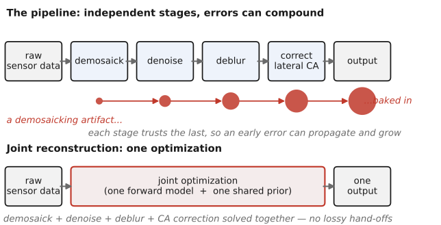
Follow a possible error on a striped shirt through a sequential pipeline. A demosaicker produces a patch of false color where its local model cannot resolve the texture. A subsequent denoiser may preserve that patch because it is spatially coherent, even while removing independent grain around it. Sharpening can then increase its contrast. Each operation can be reasonable for its assumed input while the composite result reinforces an earlier mistake. This is a reason to retain the original mosaic and its uncertainty when designing the estimator. It is not inevitable: a sequential method whose later stages model reconstruction artifacts can behave differently.
The information-flow issue is the commitment at an intermediate image. Once a stage passes only one RGB estimate onward, a later stage may have no indication that two different textures fitted the original mosaic almost equally well. It cannot reconsider that ambiguity using the raw likelihood unless the raw data or an adequate uncertainty representation remains available. A joint objective keeps those constraints active while the estimate changes. This is the useful distinction between coordinating several reconstruction operations and merely running them once in sequence.
The two orderings, made visible⧉
optionalCompare the same raw input, output domain and computation budget. Tune the sequential and joint methods separately on validation data.
Denoising before reconstruction can remove details needed for interpolation if it oversmooths them. A CFA-aware denoiser need not mix neighboring color channels, and its strength can be chosen to retain those structures.
Demosaicking first changes the noise covariance and may introduce structured artifacts. A denoiser trained or designed for this input can address some of them. Independent white-noise assumptions should not be transferred unchanged from raw samples to demosaicked RGB.
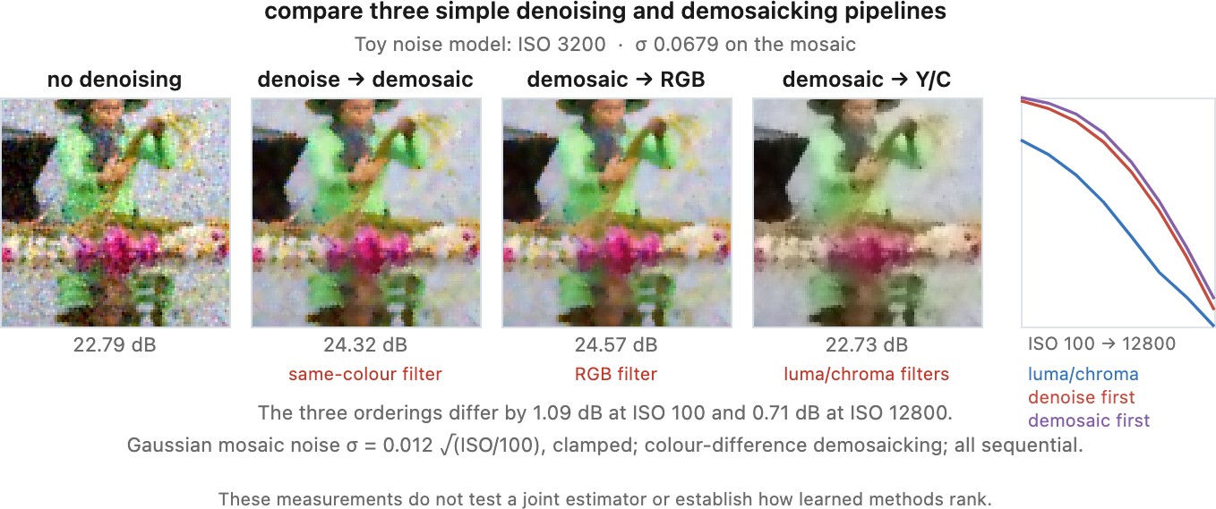
FlexISP: one energy, one prior⧉
optionalThe idea of collapsing the pipeline into a single optimization was crystallized by Heide et al. (2014) in a system named FlexISP, a flexible image-signal processor built as one energy function rather than a fixed chain Heide et al. 2014. Its architecture is exactly the inverse-problem template we have been using. On one side, a single image-formation model: a linear operator $A$ that composes all the physical steps the sensor performed (subsampling by the color-filter mosaic, blurring by the optics' point-spread function, geometric warps for lens distortion and lateral color, even the resampling of a burst of frames) into one map from the clean latent image $x$ to the raw measurement $y$. On the other side, regularization applied to the shared latent image, combining image and cross-channel structure. Recovery is the one objective $\tfrac12\lVert Ax-y\rVert^2 + \lambda\,\Phi(x)$, minimized as one large optimization.
A composite operator permits the data fit to account for several physical effects together. Operator splitting decomposes the numerical solve into manageable subproblems; it does not remove the need to define each forward operation, boundary and adjoint consistently. Chapter 13.11, Denoising as a universal prior distinguishes explicit proximal priors from arbitrary inserted denoisers.
A shared final-image prior avoids some incompatible intermediate objectives, but its accuracy remains a modeling choice. FlexISP demonstrates a flexible formulation, not a theorem that one prior always beats every stagewise pipeline.
FlexISP evaluated ADMM Boyd et al. 2011 (ADMM) and a first-order primal-dual solver, and used the latter in its reported examples. Its regularization combines BM3D Dabov et al. 2007, total variation and a cross-channel term rather than relying on a color penalty alone (FlexISP paper). Splitting the numerical work into updates does not recreate a one-pass ISP: the updates revisit one shared image and reconcile their constraints through iteration. This is why a system can contain several computational modules while still solving a joint reconstruction problem.
Joint methods and the end-to-end pipeline⧉
Where demosaicking sits in the pipeline⧉
optionalDemosaicking normally follows linearization, black-level correction, and defect handling. White balance and denoising may occur before it, after it, or jointly with it; a scalar CFA sample can already receive its channel's white-balance gain. A camera-to-output color matrix requires reconstructed channels. Nonlinear rendering and output encoding belong to the later appearance stages, as summarized in Chapter 8.12, Recap ISP, non-destructive editing.
Hardware alternatives to the mosaic⧉
Pixel shift: spending time, precisely⧉
optionalIn an ideal static scene, a four-shot cycle with one-pixel offsets can sample each scene-grid position through red, both green phases and blue. This avoids interpolating missing color components at covered interior positions. Actual fusion still needs calibration, accurate offsets, valid boundaries and motion handling.
Two patterns are in use and they buy different things. A one-pixel, four-shot cycle buys color: full color at the sensor's native resolution, direct sampling of each color at covered positions, with demosaicking removed from the pipeline entirely. A half-pixel cycle, usually eight or sixteen shots combining whole- and half-pixel steps, buys resolution as well, interleaving the sampling grids finely enough to raise the effective pixel count, which is the deliberate version of the hand tremor that Chapter 14.2, Multi-frame super-resolution exploits. Sony calls it Pixel Shift Multi Shooting, Pentax calls it Pixel Shift Resolution, OM System calls it High Res Shot, and Hasselblad calls it Multi-Shot, which tells you the market: landscape, product, and cultural-heritage work.
Commanded actuator offsets do not guarantee exact scene registration. Shake, lens distortion, actuator error and subject motion can perturb them. Fusion may reject moving regions or use a single-frame reconstruction there. Controlled pixel shift and unconstrained handheld fusion therefore share sampling principles but need not use identical algorithms.
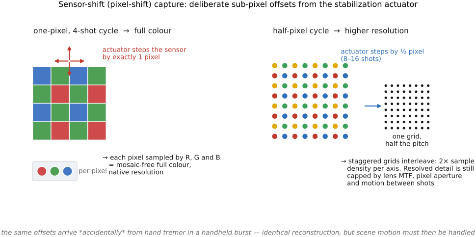
Foveon and stacked photodiodes: spending silicon depth⧉
optionalSilicon absorbs short wavelengths near its surface and long wavelengths deeper in, so three photodiodes stacked at different depths in the same pixel respond to three different, broad, overlapping spectral bands. That is the Foveon sensor (Lyon & Hubel 2002 (Foveon)): three measurements at every pixel location, no filter array, no demosaicking, with reduced CFA-specific color aliasing when all channels share the same grid. Ordinary spatial aliasing and channel-response differences remain; some stacked designs also use different sampling densities across layers. The full account of the physics is in Chapter 4.6, Sensing color: multiplexing strategies; the reason it belongs here is what it implies for reconstruction, which is that missing-color interpolation can be reduced while spectral separation and noise estimation remain necessary.
It did not displace Bayer, and the reasons are instructive because none of them is about the idea. The three depth responses overlap heavily and are not the primaries anyone would choose, so recovering colorimetric values needs a color-separation transform whose coefficients and conditioning can amplify noise: the color separation is set by silicon's absorption curve rather than by a filter someone designed. Carriers generated at one depth diffuse to another, which is crosstalk that further mixes the bands. The potential advantage is collecting useful light at several depths without a surface color mosaic. Not every incident photon is collected, however, and collection efficiency differs by layer. The resulting benefit depends on both collection and how well the overlapping responses can be separated.
The lesson generalizes past this one sensor. A measurement that captures more per pixel is only better if the mixing it introduces can be inverted without amplifying noise, which is the same conditioning argument that governs every multiplexed measurement in Part 34, Computational sensors.
Four ways to multiplex color⧉
optionalThe mosaic is a clever answer to a hard constraint (a photosite measures one number, and color needs three) but it is not the only answer, and seeing the alternatives makes clear what the mosaic trades away. Broadly, you can multiplex the three measurements in time, in space, or in depth.
- Temporal multiplexing: take three exposures through three filters, one after another. Sequential filtered acquisition was used by Sergei Prokudin-Gorskii for color photographs of the Russian Empire around 1900, shooting three plates through red, green, and blue filters. (The same idea lives on in the color wheel spun in front of a monochrome sensor.) You get three real measurements at every pixel and need no interpolation, but only for a static scene; anything that moves between exposures shows color fringes.
- Spatial multiplexing: one measurement per location, varying the color across the grid: the Bayer mosaic itself, and, not coincidentally, the strategy your retina uses (a mosaic of long-, medium-, and short-wavelength cones). Single sensor, high resolution, mature technology, at the cost of interpolation (this whole chapter), color jaggies, the resolution lost to the OLPF, and the light absorbed by the filters.
- Three sensors: split the incoming light with a prism and route it to three separate sensors, one per color (the 3-chip / 3-CCD video cameras, named after the charge-coupled device (CCD) sensor). Three real values per pixel and almost no photons wasted (the prism redirects rather than absorbs), but you pay in cost, bulk, and alignment.
- Depth multiplexing: stack the color-sensitive layers so each pixel measures all three at once at different depths: color film (tripack emulsions) and the Foveon sensor, which exploits the fact that longer wavelengths penetrate silicon more deeply. Three numbers per pixel and good light efficiency, but it needs more color processing and tends to be noisier.
These all tie back to Chapter 4.1, Linear color reproduction and CIE XYZ of the book; the takeaway is that the Bayer mosaic wins on cost, resolution, and single-sensor simplicity, and demosaicking is the computational price we pay for that win.
Demosaicking TLDR⧉
- Preserve the raw mosaic, CFA layout and origin, black/white levels, gain and saturation mask. Cropping or rotating a mosaic changes its phase. A network expecting RGGB will not interpret BGGR correctly by itself.
- Use a demosaicker matched to the sensor and noise conditions. Compare a strong classical method with a learned or joint method on fine fabric, colored edges and small text; clean-looking detail can still be wrong (Chapter 15.1, Basic traditional demosaicking, Chapter 15.2, Advanced traditional demosaicking, Chapter 15.6, Learned demosaicking).
- Model noise in the domain where reconstruction operates. Gains scale variance by their square; interpolation can introduce correlations. Joint demosaicking and denoising can help, but compare it with properly designed sequential baselines (Chapter 15.8, Joint demosaicking and denoising).
- Check calibration before tuning reconstruction: defects, autofocus-site correction, clipping, shading and chromatic displacement can create colored artifacts. Highlight recovery estimates missing signal; it cannot guarantee original color after saturation.
- Keep a documented color representation for later rendering. Learned reconstruction can coexist with exposure, white-balance and tone controls. End-to-end training does not require giving up editable stages (Chapter 15.9, Joint methods and the end-to-end pipeline).
- Treat synthetic remosaicking and unprocessing Brooks et al. 2019 (Unprocessing) as training models. They do not recreate the original sensor capture exactly. Validate on representative cameras and report input domain, reference preparation, color error and computation.
A Bayer photosite measures one filtered channel, leaving the other two to be estimated. Two classical ideas make a useful starting point: interpolate along an edge, and interpolate color differences rather than independently smoothing every channel. Estimate the more densely sampled green channel, then use it to guide red and blue. Color differences are often smoother than the channels, though saturated color edges can break that assumption. Residual interpolation Kiku et al. 2013 (residual interpolation) takes the same idea further: fit a local relationship between channels and interpolate what the fit leaves unexplained (Residual interpolation and ARI).
The frequency view explains why fine monochrome texture can turn into false color. A periodic color-filter array shifts combinations of color signals into different frequency bands. Reconstruction must separate them; when scene detail overlaps a chrominance band, the measurements admit competing color and texture explanations. That is a sampling ambiguity, and a cleaner-looking reconstruction can still choose incorrectly (Chapter 15.3, Mosaics and aliasing).
Array design changes the problem. X-Trans changes the pattern and distribution of aliases; it does not eliminate aliasing. Quad-Bayer groups like-colored sites, supporting binning and reconstruction modes with different resolution and noise tradeoffs. RGBW adds broad-band measurements while reducing the sites allocated to filtered color. Match the reconstruction to the actual array and operating mode (Chapter 15.5, Alternative color filter arrays).
Denoising and demosaicking affect one another. Denoising a raw mosaic must respect the different channels; indiscriminate neighborhood averaging mixes different measurements. Demosaicking first can turn independent sensor errors into correlated errors and can turn a noisy direction decision into a visible artifact. Joint methods use the mosaic and its noise model together. They can help avoid this propagation, but still impose a prior and can lose detail or fail on unfamiliar data. A sequential baseline designed for the correct domains remains a useful comparison (Chapter 15.8, Joint demosaicking and denoising).
For a learned method, realistic supervision matters as much as the network. Smooth regions dominate random crops, while the difficult cases are fine fabric, roof tiles, fences, and colored edges. Include those cases during training and evaluation. Synthetic remosaicking provides convenient pairs, but a processed reference may already contain demosaicking artifacts. Unprocessing approximately reverses encoding and rendering to construct raw-like training examples; it cannot undo clipping or retrieve information discarded by the original pipeline (Chapter 15.6, Learned demosaicking, Chapter 15.11, Synthetic data, unprocessing, and raw reconstruction).
Inspect the artifacts separately from an average score. CPSNR can summarize reference error while hiding a small region of conspicuous zippering. Color and spatially filtered color-difference measures answer complementary questions; none replaces looking at the difficult structures. Use the same color representation, crop, alignment, and reference preparation when comparing methods.
The surrounding pipeline also matters. Learned raw reconstruction can feed a documented color representation with adjustable exposure, white balance, and tone controls. Joint training does not require an uneditable raw-to-JPEG network. Preserve the intermediate quantities a photographer or later rendering stage needs (Chapter 15.9, Joint methods and the end-to-end pipeline).
Alternative capture hardware changes which colors are missing. Pixel shift can measure more color samples at corresponding scene positions when the scene stays still. Layered sensors separate spectral responses through depth but still need color unmixing. Multi-sensor optical systems trade alignment and hardware complexity for simultaneous measurements. These alternatives spend time, space, or optical complexity to reduce the spatial sampling compromise of a mosaic (Chapter 15.12, Hardware alternatives to the mosaic).
Holography⧉
Lippmann and Gabor: recording the wave⧉
optionalThe intellectual root is again Chapter 31.2, Light field cameras, the same physicist behind integral photography. In 1891 Gabriel Lippmann invented interference color photography Lippmann 1891, which won him the 1908 Nobel Prize. He recorded color not with dyes but with standing waves: light reflecting off a mirror behind the emulsion interfered with the incoming light, laying down microscopic layers in the film at spacings set by the light's wavelength, so the developed plate reconstructed color by reflecting back exactly those wavelengths. It was the first photographic process to record information in the standing-wave structure of light rather than in intensity alone, the conceptual seed of capturing phase.
Holography proper was invented by Dennis Gabor in 1948 Gabor 1948, for which he received the 1971 Nobel Prize. (He was trying to improve electron microscopy, not to make 3-D pictures; the 3-D display application came later.) Gabor's insight: bring the light from the object together with a coherent reference beam at the recording plate, and let them interfere. Where the two waves arrive in phase they reinforce (bright); where they arrive out of phase they cancel (dark). The resulting pattern of fine fringes is an intensity pattern an ordinary plate can record, but because the fringe positions depend on the phase difference between object and reference at each point, that intensity pattern secretly encodes the object wave's phase as well as its amplitude. The phase difference appears in a recordable intensity. With object field $U_o$ and reference field $U_r$,
The cross term carries their relative phase. A single intensity sample does not uniquely determine a general complex field; the known reference and the holographic encoding geometry make separation and reconstruction possible.
On replay, illuminate the developed fringe pattern with the reference beam again, and the fringes act as a diffraction grating. They bend the reference light by exactly the angles that reconstruct the original object wave. The wavefront that leaves the hologram is (to good approximation) the very wavefront the object once sent. Within the reconstructed aperture, wavelength band, and viewing zone, it can reproduce the corresponding visual cues: look from the left and you see the object's left side; move your head and it shows full, continuous parallax; and your lens accommodates to the true depth of each virtual point, because the reconstructed wavefront has the correct curvature.
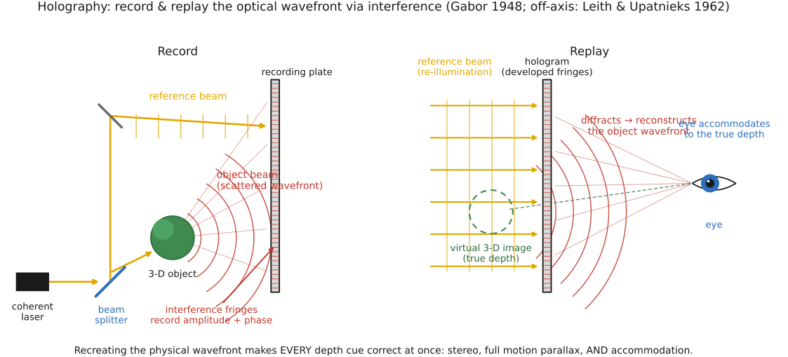
Recap: big lessons in this lecture
Strip away the color filter and a sensor is monochrome at the pixel: each photosite reports a single number, a signal proportional to detected photoelectrons within its operating range, not a color. The three (or more) values that color needs must therefore be multiplexed along some other axis: over space (a color-filter array such as Bayer, paying with resolution and a demosaicking step), over time (sequential color filters, paying with motion robustness: the old color-wheel and many scientific cameras), across multiple sensors (a beam-splitter prism feeding three chips, the 3-CCD video camera, paying with bulk and cost), or over depth (wavelength-dependent absorption in stacked photodiodes, the Foveon, paying with noise). The choice determines which measurements are simultaneous and co-located. The same constraint shapes the eye, whose three cone types sample color over space at the retina (L3.1, L3.6).
Edge-directed demosaicking is a first, very concrete instance of a theme that returns throughout the book: adapt the operation to the local structure of the image rather than applying the same fixed filter everywhere. Here the structure is an edge and the adaptation is choosing the interpolation direction; later, in edge-preserving filtering and denoising, the same instinct (use the similarity between pixels to decide how much they should influence each other) becomes the bilateral filter and the idea of affinity. Whenever a fixed linear filter blurs across something it should have respected, the cure is to look at the data first.
Channel differences are often smoother than luminance-like structure, which makes guided reconstruction useful. Preserve that distinction as an image model rather than a law: fine color texture and saturated boundaries can break it.