Lecture Notes 4 — Color⧉
Course notes cut from Computational Photography, an AI-powered Slopendium for this lecture. Each section links back to its home in the book; sections marked optional go beyond what the lecture needs.
Contents · 32 sections on this page, from 9 chapters of the book
Titles jump to the section below; ↗ opens it in the book.
Light and optics⧉
Light: rays, waves, and the spectrum⧉
optionalThere is no single right answer to "what is light." Physics offers three models (Figure 2.1.1), and the trick is to pick the one that makes the question at hand easy. When we want to know where light goes, through a pinhole, a lens, or off a mirror, we treat it as a ray, a straight line obeying simple geometry. When we want to understand color, diffraction, or interference, we treat it as a wave, a periodic disturbance with a wavelength. And when we want to count light precisely, which is what ultimately limits image quality, we treat it as a stream of photons, discrete particles whose random arrival creates noise. The three pictures describe different aspects or approximations of the same physics.
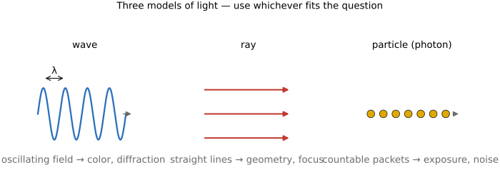
The wave picture and the spectrum. Light is an electromagnetic wave, a coupled oscillation of electric and magnetic fields that travels through vacuum at a fixed speed $c \approx 3 \times 10^{8}$ m/s (about 300,000 km/s, and slower by a factor $1/n$ inside a medium of refractive index $n$). A single-frequency, or monochromatic, wave is characterized by one wavelength $\lambda,$ the distance between successive crests, or equivalently by its frequency $\nu,$ the two tied by
Visible light occupies a narrow band, roughly 400 nm (violet) to 700 nm (red), a small part of the electromagnetic (EM) spectrum that also includes radio, microwave, infrared, ultraviolet, X-rays, and gamma rays, all the same physics, differing only in wavelength (Figure 2.1.2). "Visible" is a fact about our eyes, not about our cameras: a standard silicon sensor responds to wavelengths the eye cannot see, into the near infrared beyond 700 nm and, with the right optics, into the ultraviolet below 400 nm, and computational photography can put that extra reach to work (Sensors).
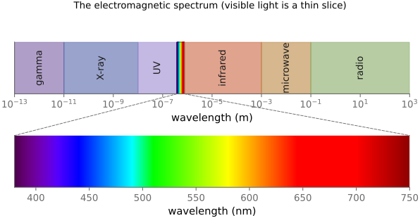
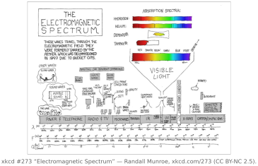
Most light is not monochromatic, however. A general wave is a superposition of many wavelengths, and what characterizes it is its spectrum: the distribution of energy over wavelength. That is, each wavelength has a given amount of energy, and this distribution characterizes the physical color of light. Physical color is different from the notion of color as perceived by humans, and the link between the two is fundamental in imaging; it is developed in Chapter 3.2, Perceptual color and trichromatic vision.
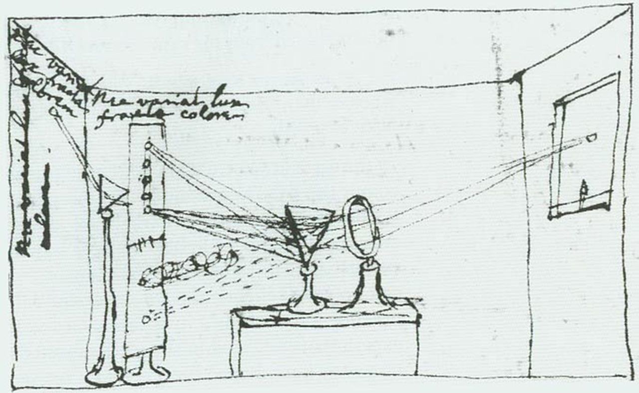
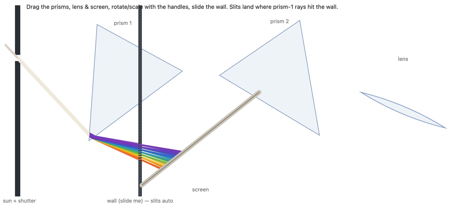
Newton's prism. Newton demonstrated the decomposition of white light into its spectrum. Pass a beam of white sunlight through a glass prism and it fans out into the full spectrum: the rainbow band of pure colors. The lesson is that white light is not a pure thing being "stained" by the glass; it is already a mixture of all wavelengths, and the prism merely bends each wavelength by a different amount, spreading the mixture out. Newton proved this with his experimentum crucis (Newton 1704 (Opticks)): he isolated one pure color from the spread and sent it through a second prism, and it did not split further. The pure colors are the irreducible ingredients; white is their sum (Figure 2.1.4).
 Isaac Newton (1642–1727) needs little introduction, but the prism is only the start of his presence in this book. The spectrum he split from white light is the physical basis of all the color science to come, and his Opticks established that color lives in the light, not the object. His corpuscular view of light competed for a century with the wave picture: both, we now know, are needed. On the mathematics side we still run Newton's method (step by the inverse curvature, $H^{-1}\nabla f$) whenever a solver wants second-order convergence, and the Gauss–Newton refinement sits at the heart of feature tracking and bundle adjustment. Portrait: James Thornhill after Godfrey Kneller, 1689, public domain (via Wikimedia Commons).
So a spectrum is simply a function: power plotted against wavelength, $S(\lambda)$. You can think of it as an infinity of channels, one per wavelength.
Light, and the physical color it carries, is described by a spectral distribution: the power it carries at each wavelength, a function $S(\lambda)$. One wavelength is a single pure color; real light is a weighted mix of all of them. Everything downstream (how a prism fans light out, how a surface reflects it, how a sensor or an eye turns it into a perceived color) starts from this per-wavelength power.
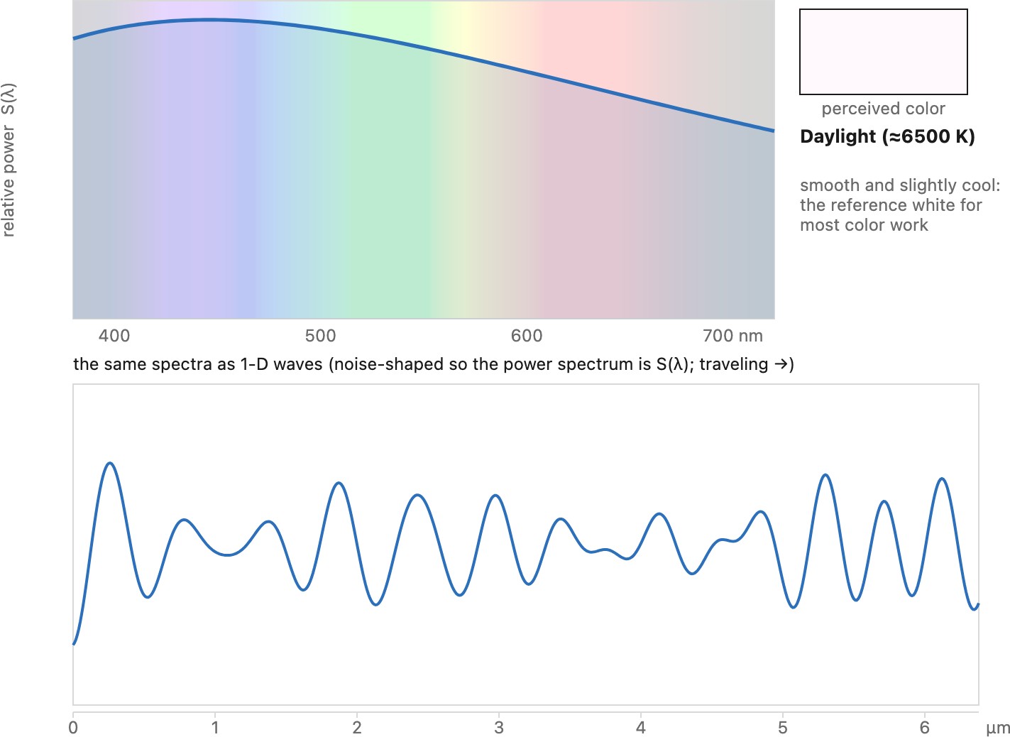
Spectra come in two broad flavors. A smooth spectrum varies gently with wavelength: daylight, an incandescent bulb, the glow of any hot body. A spiky spectrum piles its power into a few narrow lines with little in between: a fluorescent tube (sharp mercury lines on a faint phosphor background), many cheap LEDs, a sodium street lamp, a laser. As we will discuss, spiky illuminants tend to be bad for photography because they single out a few wavelengths: their color rendering is poor (skin tones and saturated fabrics shift unpredictably), they defeat a single white-balance correction, and a scene under them can look sickly even though a meter calls the light white. Smooth, broadband light (daylight, tungsten, good full-spectrum LEDs) is forgiving; spiky light is treacherous. We return to this with white balance, color rendering, and the design of a camera's color filters.
Rays. The most useful everyday picture ignores the oscillation entirely and treats light as rays: straight lines along which light carries its energy. In a uniform medium a ray travels perfectly straight and changes direction only when it meets a surface, bending by refraction as it passes into glass or water and bouncing by reflection off a mirror. This is geometry rather than wave mechanics: to find where an image forms, you follow rays through the optics and see where they cross. It is a simplification, valid when the wavelength is tiny compared with the apertures and features the light meets, so that diffraction and interference are negligible, but it is the workhorse of this book. The overwhelming majority of what follows, image formation, focus, depth of field, exposure, nearly all of the optics, runs on ray optics, and often on an even simpler version of it, the paraxial thin-lens approximation. We reach for the wave picture only where it is unavoidable, for diffraction, interference, and the resolution limit; the rest of the time, light is rays.
Photons. The third picture is granular: light arrives in discrete packets called photons, and a detector, a camera pixel or a cell in the eye, absorbs them one whole photon at a time. Wave and photon are the same light seen two ways. The wave tells you where the light goes and how bright it is, and its intensity (the square of the amplitude) is really the density of photon arrivals; the photon is what actually gets counted. Each photon's energy is set by the wave's frequency, $E = h\nu$ (with $h$ Planck's constant), so frequency is color: a blue photon (high frequency, short wavelength) carries more energy than a red one. We are simplifying here by giving each photon a single frequency, one pure wavelength; a real photon is a short wave packet with a small spread of wavelengths, but the one-frequency-per-photon picture is all photography needs. In this view the oscillation is not something a lone photon waves about in flight, it is the wave property that fixes the photon's color and energy, while the wave's amplitude sets how many photons show up. And because photons arrive at random, counting a finite number of them is inherently noisy, which is the shot noise that ultimately limits how clean an image can be.
How light is created⧉
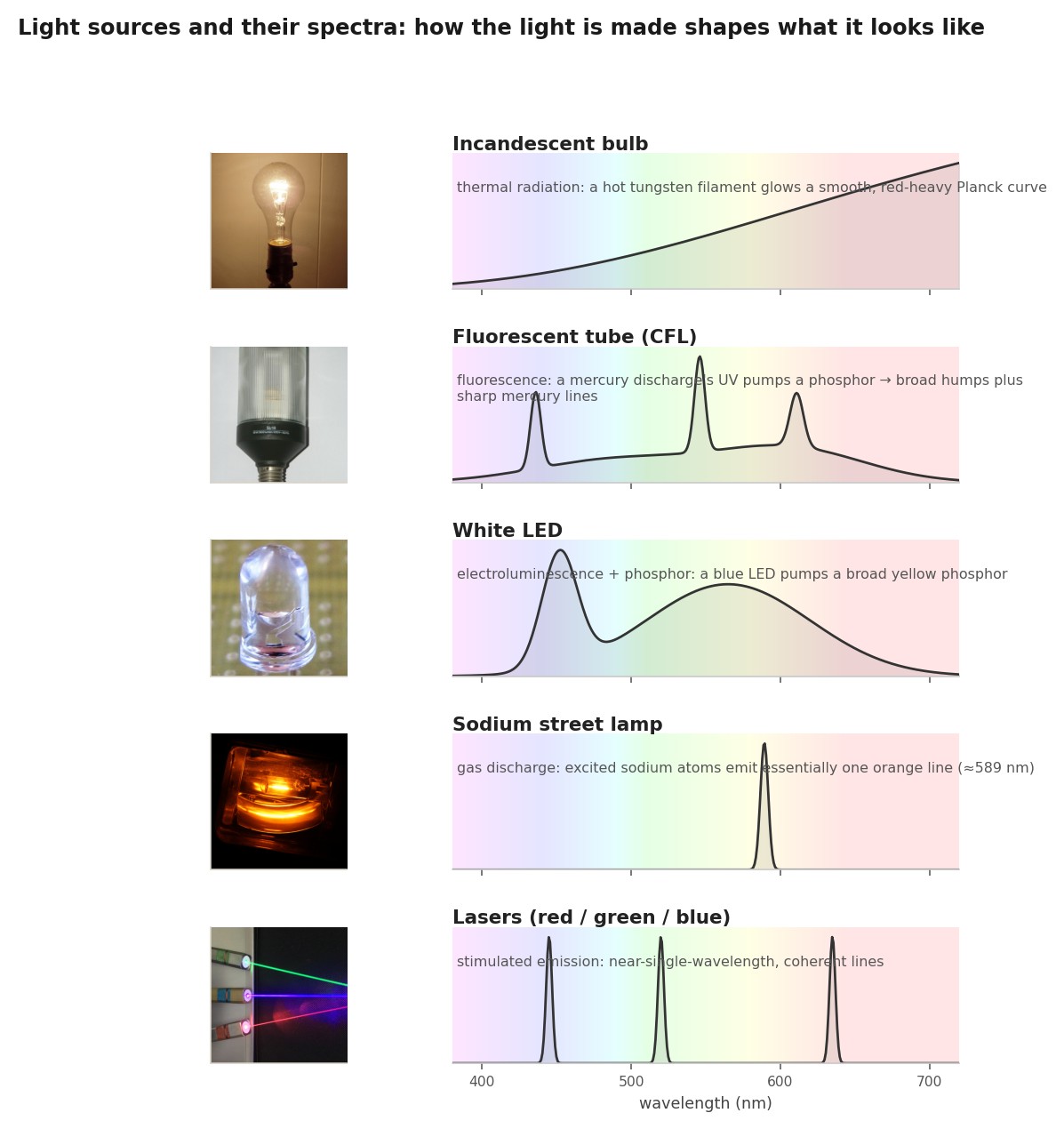
optionalWhy do those spectra look the way they do? Accelerating charges radiate in classical electrodynamics; but the sources we photograph fall into a handful of physical processes, and each one stamps a characteristic spectrum. Knowing the mechanism tells you, before you ever meter the scene, whether a light will be smooth or spiky, warm or cool, and forgiving or treacherous to correct (Figure 2.1.7).
Each of those spectra is the fingerprint of a different way of making light, and it helps to watch the mechanisms actually run (Figure 2.1.8).
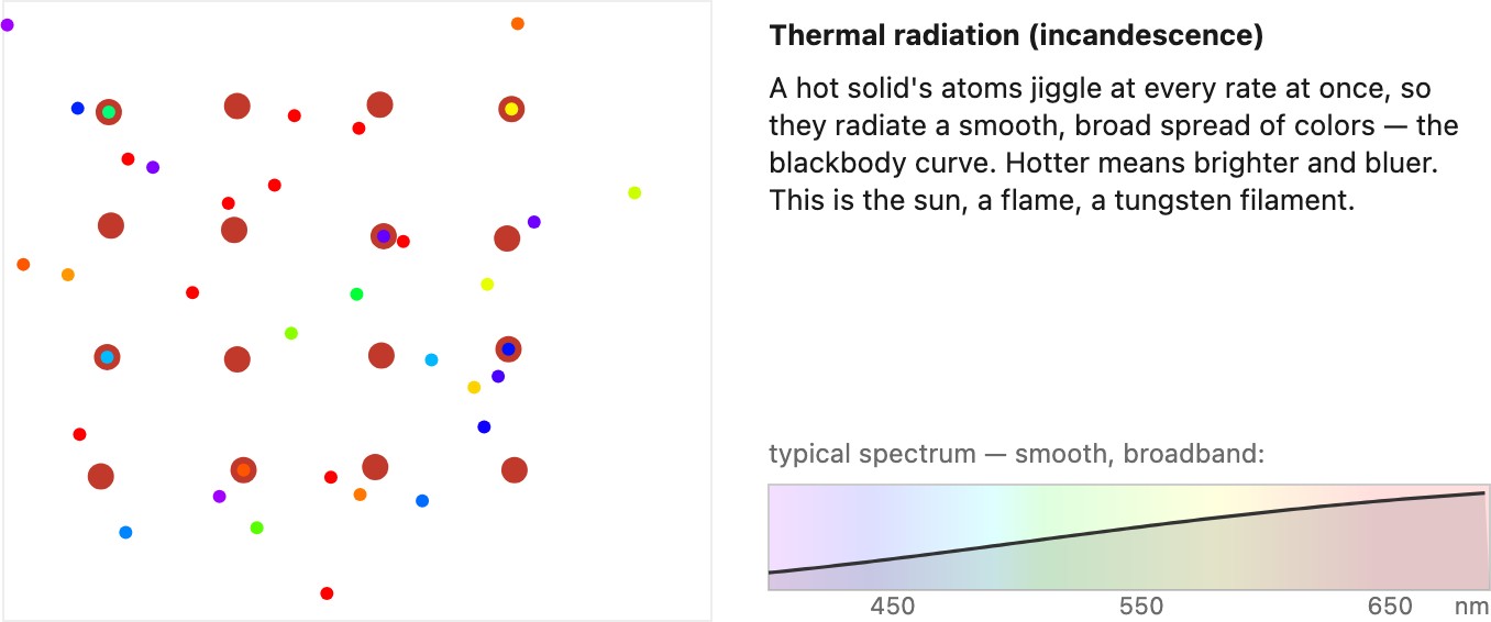
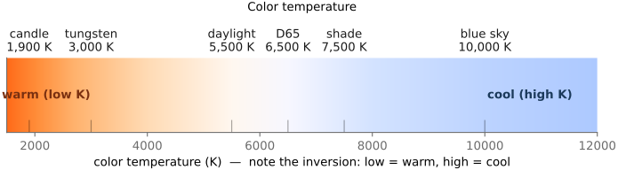
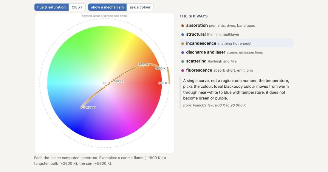
Thermal radiation (incandescence). Heat anything enough and it glows. An ideal blackbody emits a smooth, broadband spectrum set by temperature alone. A real hot surface modifies it by its wavelength-dependent emissivity: as the object heats, the curve brightens and its peak slides from red toward blue, the sequence a heated iron bar runs through (dull red, orange, yellow, white, finally bluish). The sun (a ~5800 K surface), a tungsten filament (~2800 to 3200 K), and a candle flame (sooty, ~1800 K) are all this same physics at different temperatures. That single controlling number is color temperature, quoted in kelvin (K): the one-number handle on the color of a light (Figure 2.1.9). The convention runs opposite to everyday usage: low color temperatures (~3000 K) are warm and orange-ish, high ones (~6500 K and up) are cool and bluish. It anchors the standard reference illuminants, chiefly D65 (≈6500 K, a model of average daylight and the basis of most color standards) and tungsten (≈3200 K, the warm glow of an incandescent bulb). Thermal sources are always smooth and always red-heavy at the temperatures a filament can survive, which is why incandescent light looks warm; it is also wasteful, since most of the radiated power is invisible infrared heat rather than light. A halogen bulb is an incandescent filament with a halogen gas that redeposits evaporated tungsten back onto the wire, letting it run hotter (whiter, more efficient) and last longer, but it is still a hot filament throwing off a Planck curve.
Not every source is a blackbody, though, so "white light" is not a single thing. Because the stimulus reaching the eye is the product $S(\lambda)\rho(\lambda)$ of illuminant spectrum and surface reflectance, the same scene sends genuinely different colors to the eye under noon daylight, sunset, tungsten, or a fluorescent tube. Fluorescent and gas-discharge lamps in particular emit spiky, non-blackbody spectra (their mechanisms are below), so they are not well described by a single color temperature and render some colors poorly. Undoing that shift so a photograph looks neutral is white balance, developed in Chapter 4.1, Color space 101.
Gas discharge (atomic emission lines). Run a current through a low-pressure gas and its atoms are kicked into excited states; each time an electron falls back it emits a photon at one precise wavelength, fixed by the spacing of that atom's energy levels. The result is a spiky spectrum of sharp lines with darkness in between. A low-pressure sodium street lamp is the extreme case: nearly all its light sits in a single orange doublet near 589 nm, which makes it very efficient but renders every color as a shade of orange-gray. Mercury vapor emits a few blue-green lines plus a lot of ultraviolet; neon glows red. These line spectra are the treacherous illuminants of the previous section: a camera's three filters cannot reconstruct what was never there between the lines.
Fluorescence (down-conversion). Line emission alone makes poor white light, so the fluorescent tube adds a trick: coat the glass with a phosphor that absorbs the mercury discharge's ultraviolet and blue and re-emits it as a broad glow at longer wavelengths (the Stokes shift, the same fluorescence discussed for surfaces below). The visible result is broad phosphor humps with the residual mercury lines still poking through, which is why a fluorescent spectrum is broad and spiky at once. This is the general recipe for turning invisible or narrow light into usable white: pump a phosphor and let it fluoresce.
Electroluminescence (LEDs). In a light-emitting diode, current drives electrons and holes together across a semiconductor junction, and radiative recombination releases a photon whose energy is set by the material's bandgap. That gives a fairly narrow band, a few tens of nanometers wide, and it does so far more efficiently than heating a filament. The catch is that one junction makes one color: a bare LED is red, or green, or blue, not white.
Making white from LEDs. There are two ways to build a white LED, and they mirror the two ways of making any white light. The first is an RGB triplet: put red, green, and blue LEDs side by side and let the eye sum them. The mix looks white and is electronically tunable, but its spectrum is three separated humps with gaps between, a metameric white with mediocre color rendering, and each color's brightness drifts differently with temperature and age, so the white wanders. The second, and now dominant, way is blue pump plus phosphor, which is fluorescence again: a bright blue LED excites a yellow phosphor that fluoresces over a broad band, and the leaked blue plus the re-emitted yellow add up to white. It is cheap and reliable, but the raw version has a dip in the cyan and weak deep reds (a cool, sometimes harsh white); warm, high-fidelity LEDs add a red phosphor to fill that gap. The spectra of both a phosphor LED and a fluorescent tube appear in Figure 2.1.6.
Stimulated emission (lasers). One source stands apart. In a laser, an excited medium is made to emit in step, so the light is essentially a single wavelength and coherent (developed in the coherence section below). Lasers rarely light a scene directly, but they are the engine behind projectors, lidar, and the structured-light patterns used for depth sensing, and their coherence is what makes speckle and holography possible.
The thread through all of this: the emission mechanism fixes the spectrum, and the spectrum, smooth or spiky, is what decides how faithfully colors render and whether a single white-balance correction can ever set them right.
A second thread runs through this too, about where in the spectrum the energy lands. An incandescent bulb is mostly a heater: the bulk of its radiated power falls in the infrared, and only a few percent comes out as visible light. Modern sources reverse that. An LED or a fluorescent tube deliberately concentrates its emission inside the visible band, which is exactly why they are so much more efficient, an LED bulb makes the same visible light for a fraction of the wattage. That is the good news, and it is why they have taken over. The catch is for the sensor: silicon detectors keep responding well past 700 nm into the near infrared, where the eye sees nothing, and that near-IR sensitivity can be genuinely useful (low-light assist, some depth and material tricks, the near-IR imaging discussed with the sensor). But under efficient modern lighting there is simply very little near-IR light in the scene to work with, because the source has been engineered not to waste any there. The old, wasteful incandescent world was, ironically, a strong near-IR illuminant; the efficient one is nearly dark outside the visible. We return to this when we look at what sensors can see beyond the visible (Sensors).
Light-matter interaction is largely resonance⧉
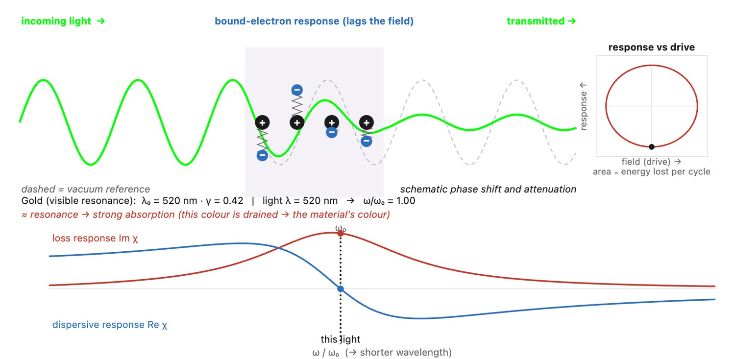
optionalWhy does light slow in glass at all, why does the index of refraction always depend on wavelength, and why do different materials attenuate different wavelengths? It all comes down to vibration and resonance of the particles that make up matter. The wave's oscillating electric field drives the bound charges in a material, such as atoms, molecules, and electrons bound to nuclei, and like any spring-loaded mass each has a natural frequency it most readily oscillates at. This can be modeled as a so-called Lorentz-oscillator, and almost everything optical follows from it. Near a resonance frequency, the driven charges swing hard and the material absorbs strongly, draining those wavelengths from the light; the wavelengths a material happens to absorb (and so remove from what it transmits or reflects) are exactly what give it its color. The same driven-charge picture runs far below light too: a microwave oven cooks by driving the water molecules in food with an oscillating field they cannot quite keep up with, and that lag turns into heat (dielectric loss, the low-frequency cousin of optical absorption). Away from resonance the charges still respond, just out of step, and that lag is what slows the wave, so the refractive index $n$ is itself a resonance effect. Because each wavelength sits a different distance from the nearest resonance, $n$ varies with wavelength; this is dispersion, $n(\lambda)$, and it is behind the prism fanning out a spectrum (Figure 2.1.15), the colors of a rainbow, and the chromatic aberration that plagues real lenses. That consequence matters: because every glass disperses, a simple lens focuses blue and red at slightly different distances, and dispersion goes on to shape much of the challenge of lens design: the whole craft of combining crown and flint glasses into achromatic and apochromatic doublets, and the modern fight against chromatic aberration in fast lenses, exists to fight exactly this $n(\lambda)$ (developed in the Optics part). The resonance picture can be explored directly (Figure 2.1.18): the bound electron is driven at different frequencies, and the absorption peaks at resonance while the refractive index swings through its normal-then-anomalous dispersion.
The refractive index is not a constant: $n(\lambda)$ depends on wavelength: in ordinary glass it rises toward the blue, so blue bends more than red. Because of this you cannot route every wavelength the same way with a single refraction: a prism fans white light into a spectrum, a raindrop makes a rainbow, and a simple lens focuses blue and red at slightly different distances: chromatic aberration. Much of the craft of lens design (combining crown and flint glass into achromatic and apochromatic groups) exists to fight this one fact. Dispersion is not a defect of cheap glass; it is built into how matter and light interact.
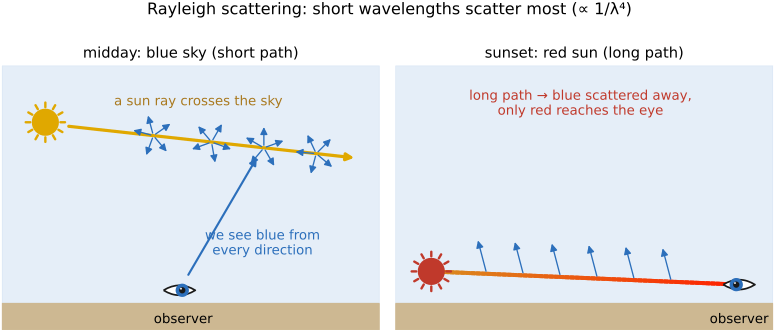
Both follow from Rayleigh scattering: air molecules are much smaller than the wavelength of light and scatter short (blue) wavelengths far more strongly than long (red) ones: the scattered fraction grows as $1/\lambda^4$, so blue (≈450 nm) scatters roughly ten times more than red (≈650 nm). At midday the sunlight takes a short path through the atmosphere; the blue it sheds is scattered out in every direction and reaches your eye from all over the sky, so the sky reads blue while the sun stays roughly white. At sunset the light skims a long, grazing path through the air; by the time it reaches you almost all its blue has been scattered away, and mostly orange and red survive, so the sun and the clouds near it redden (Figure 2.1.19). When the scattering particles are large compared to the wavelength (water droplets in fog or cloud), every wavelength scatters about equally (Mie scattering), which is why clouds and haze are white or gray, not blue. Minnaert, The Nature of Light and Color in the Open Air One caveat the physics alone hides: the color you finally see is not in the scattered light by itself: "blue" and "orange" are your cones' verdict on these spectra, so the apparent color of the sky depends on the visual system reading it as much as on the scattering. The same sky spectrum read by a different eye is a different color, vividly so across species (→ the cross-species sky figure in Chapter 3.2, Perceptual color and trichromatic vision Weiss & Springer 2026 (color of the sky for a non-human)).

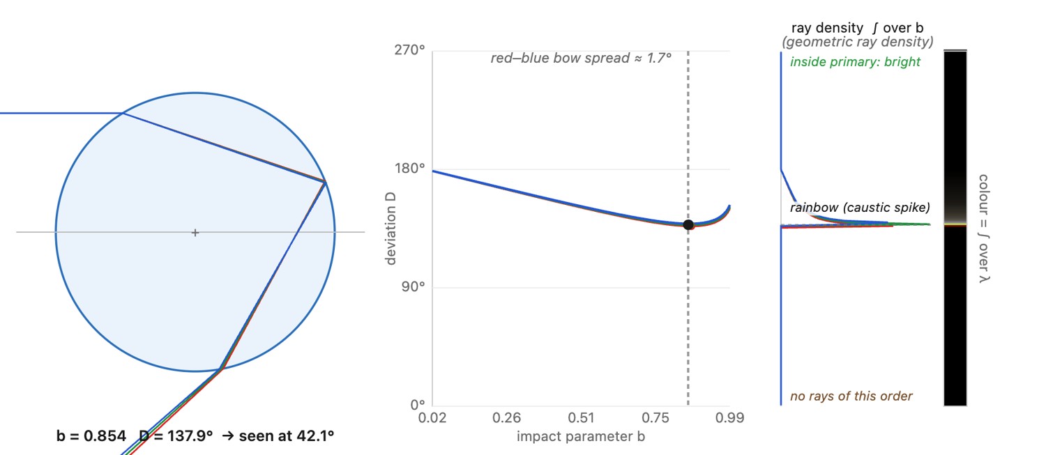
A rainbow is a caustic, a place where rays concentrate. It is tempting to explain it as "dispersion, like Newton's prism," but dispersion alone is not a rainbow: a prism merely fans white light into a spread, and a spread is not a bright arc pinned at a fixed angle. The brightness and the fixed 42° angle come from the geometry of the sphere; dispersion only supplies the colors. Each falling raindrop is a tiny sphere, and sunlight refracts in, reflects once off the back, and refracts out again (Figure 2.1.21, left).
Slide the entry point across the drop (the impact parameter) and the total deviation of the exiting ray sweeps down to a minimum (about 138° for water) and turns back up. Near that minimum the deviation is stationary, so rays entering at many different points all leave in almost the same direction: they bunch up, and that pile-up is the bright arc, seen at $180°-138° \approx$ 42° from the antisolar point (Figure 2.1.21, right). This is why the single internal reflection is essential, and why a ray that only refracts in and out, with no bounce, makes no rainbow at all: with two refractions only, the deviation grows monotonically with the impact parameter and never turns around, so there is no stationary angle for light to concentrate at. The primary bow is the one-bounce caustic at 42°; the fainter, color-reversed secondary bow is the two-bounce caustic, its own minimum putting it at about 51°. Dispersion then sets the color order: because $n$ is a touch larger toward the blue, each color's caustic sits a degree or so from its neighbors, fanning the bunched light into the ordered band we see.
Between the two bows sits a conspicuously darker strip of sky, Alexander's band (named for Alexander of Aphrodisias, who described it around 200 AD). Its darkness follows directly from the caustic story: one-reflection light only ever emerges at 42° or less (it piles up at 42° and scatters out to fill the sky inside the primary bow), while two-reflection light only emerges at 51° or more, outside the secondary. The 42°–51° gap between them receives almost no rainbow light from either path, so it reads as a dark band, with brighter sky on both sides. You can see the whole story in a real double bow over Loch Ness (Figure 2.1.24): bright primary, fainter reversed secondary outside it, the dark band between, and the noticeably brighter sky inside the primary.
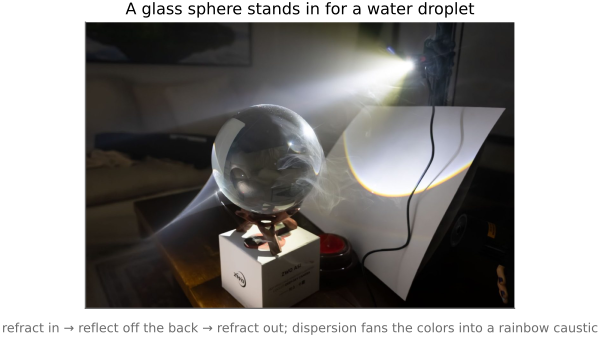
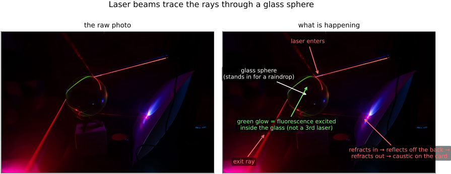
You can run the whole experiment on a workbench with a clear glass sphere standing in for a raindrop (Figure 2.1.22): a bright beam refracts in, reflects off the back, and throws a little rainbow caustic onto a card. Send narrow laser beams through the same sphere in a hazy room and the rays themselves become visible (Figure 2.1.23): you can watch each beam refract in, bounce off the back, and refract out: the exact refract–reflect–refract path the diagram traces. The rainbow in the sky is just this single-drop geometry, summed over a skyful of drops. Minnaert, The Nature of Light and Color in the Open Air

Scattering and absorption in media. The same physics that paints the sky operates at close range whenever light travels through a participating medium such as fog, haze, smoke, or water. Light is scattered out of its straight path and absorbed along the way, so distant objects lose contrast and take on the color of the medium (the bluish veil of haze, the green-blue cast underwater). When light scatters only once before reaching the camera the effect is mild; multiple scattering through thick fog washes the scene out entirely. Undoing this (dehazing and de-weathering) is a recurring computational-photography problem, and it is built on exactly the scattering model sketched here.
The color of objects: illumination times reflectance⧉
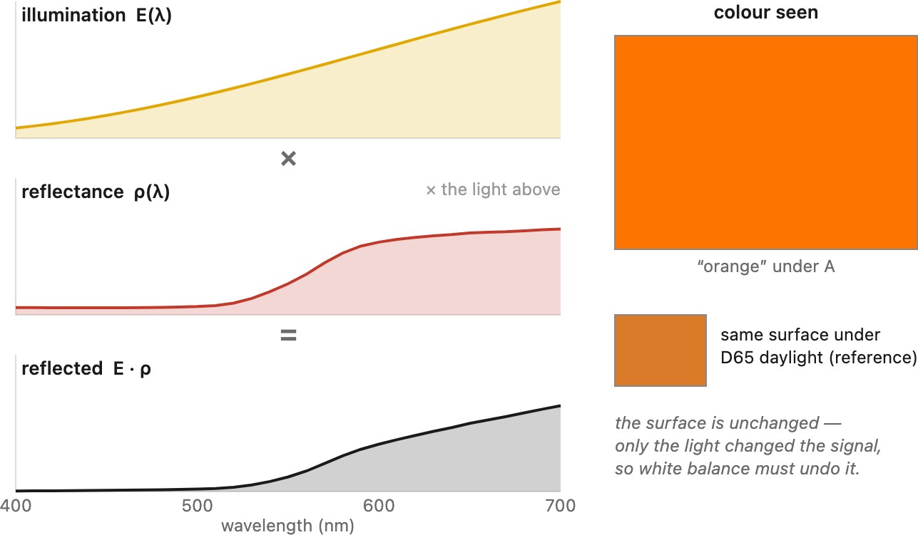
Most ordinary photographed objects emit negligible visible light of their own; they only reflect whatever light falls on them. So the color that reaches your eye is the result of two spectra multiplied together, wavelength by wavelength:
Here $S(\lambda)$ is the illuminant (the spectrum of the light source actually present) and $\rho(\lambda)$ is the surface's spectral reflectance, the fraction of light it sends back at each wavelength. Reflectance is the object's intrinsic, fixed signature: the apple's $\rho(\lambda)$ is high in the reds and low in the greens and blues, whatever the lighting. Illumination is whatever happens to be shining. Their per-wavelength product is what leaves the surface and reaches the eye (Figure 2.1.28). A red apple under white light reflects mostly red; the same apple under pure green light has almost nothing to reflect and looks nearly black, because there is no red illumination for its reflectance to act on.
This multiplicative entanglement is consequential, and it is the first instance of a principle that runs through the whole book.
Much of imaging is multiplicative, not additive. The light reaching the eye is illumination times reflectance; contrast is a ratio of intensities; a shadow darkens a region by a factor, not by subtracting a constant. Because the structure is multiplicative, the natural tools are multiply, divide, and log, not just add. This is why, again and again, we will work with ratios and with logarithmic encodings rather than raw linear values. It is also why white balance is hard: to recover an object's true color we must divide out the unknown illuminant $S(\lambda)$ from the product $C(\lambda)$, undoing a multiplication we never observed directly. (The additive counterpoint, light from different sources adding, and what it means for choosing an encoding, comes in Color technology.)
Why this multiplicative structure matters so much is a question the rest of the book keeps answering. Our visual system does not care about the illumination for its own sake. It cares about objects, about the reflectance $\rho(\lambda)$ that tells it what a thing is and whether it is food, a face, or a threat. So the brain works hard to discount the illuminant, factoring the product $C(\lambda)=S(\lambda)\,\rho(\lambda)$ back apart to recover the reflectance and hold an object's apparent color and lightness steady as the light changes. That discounting is the perceptual machinery of lightness and color constancy, studied in Human vision and color, and a camera has to imitate it deliberately, which is exactly what white balance does. Much of imaging is this running effort to see past the illumination to the reflectance underneath.
Where color comes from⧉
optionalThat fixed reflectance $\rho(\lambda)$ (and color in nature more broadly) is produced by only a handful of physical mechanisms that behave very differently in a photograph.
- Pigments: selective absorption. The common case, and at bottom it is all resonance: molecules or crystals whose bound electrons resonate at, and therefore absorb, particular wavelengths, the very same driven Lorentz-oscillator picture from the light-matter discussion above (Figure 2.1.18), leaving the off-resonance wavelengths to be reflected or transmitted. The color you see is simply what is left once the resonant wavelengths are drained away. Chlorophyll's green, the apple's red anthocyanins, paint, dye, ink, the melanin in skin and hair are all pigments. An ideal matte pigmented surface has a view-independent color described by a single reflectance function $\rho(\lambda)$, which is exactly why it photographs as a stable, matte color a camera can capture and a printer can match.
- Structural color: interference and diffraction. Color produced not by any pigment but by micro-geometry on the scale of the wavelength of light, which makes some wavelengths interfere constructively and others cancel. A single thin film colors soap bubbles, oil slicks on a wet road, and anodized metal; a stack of many wavelength-scale films (multilayer interference) gives the brilliant blue of a Morpho butterfly and the metallic sheen of a jewel beetle; a periodic 2-D or 3-D lattice (a photonic crystal) colors a peacock feather's barbules and an opal; and a diffraction grating colors a CD, holographic foil, and some beetles. Many structural colors are iridescent: the hue shifts with viewing and lighting angle, because it comes from path-length differences. Such structural color is strongly directional: a genuinely spectral version of the next section's BRDF, not a single albedo, and the reason it is so hard to reproduce in print, which has no angle to give back.
- Emission. Some things make their own light rather than reflecting it: a glowing filament or the sun (incandescence, fixed by temperature → color temperature, under How light is created above), a fluorescent dye or a firefly (luminescence). Emission adds light to the scene instead of multiplying the illuminant.
- Scattering. Wavelength-selective redirection by tiny particles. Rayleigh scattering paints the sky blue and the sunset orange (sidebar above), and the very same effect gives blue eyes and some birds their blue without a speck of blue pigment.
For photography the split that matters is pigment versus structural: a matte pigment can often be approximated by a fixed $\rho(\lambda)$, whereas an iridescent structural color changes as you move, so a single frame freezes only one slice of it and a flat print loses the iridescence entirely (Figure 2.1.30).

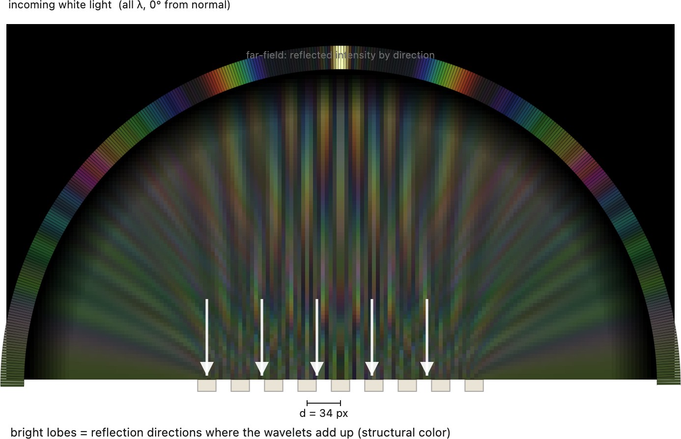
Structural color comes from interfering wavelets, which you can watch directly (Figure 2.1.32). A periodic microstructure re-radiates a wavelet of the incoming light from each of its elements; where those wavelets' paths line up they reinforce into bright lobes and elsewhere they cancel, and because the lobe directions depend on the ratio of wavelength to structure spacing, a fixed viewing direction sees the color shift as either changes. That angle-dependence is the iridescence, and it is why structural color cannot be captured as a single reflectance.
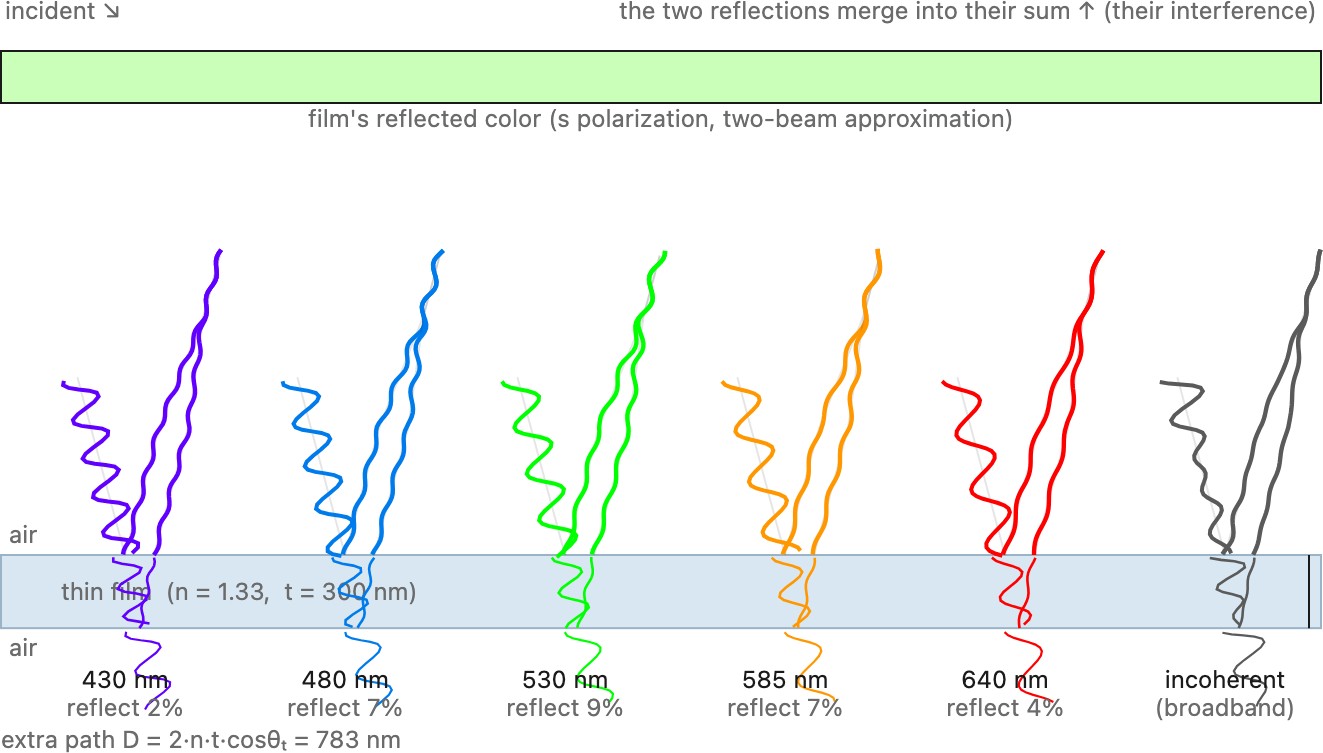
The other common route to structural color is a thin film rather than a periodic array: a single transparent layer, the wall of a soap bubble or the sheen of oil on water, reflects light from both of its surfaces, and those two reflections interfere by an amount set by the film's thickness and the viewing angle (Figure 2.1.33). Constructive reflection depends on the optical path difference and on phase shifts at the two interfaces; with one reflection phase reversal, a half-integer-wavelength optical path difference reinforces the reflection. As the film thins or you tilt it the reinforced color marches through the spectrum, which is the shifting sheen of a soap bubble about to pop.
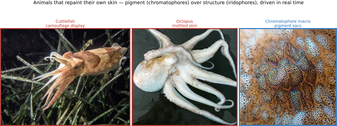
Every mechanism above is fixed once the material is made: a pigment absorbs the same wavelengths today and tomorrow, and a butterfly's scales keep their spacing for life. Cephalopods (octopuses, squid, and cuttlefish) break that assumption. They run two of this section's mechanisms at once and steer both in real time, changing color and pattern in a fraction of a second. The pigment layer is built from chromatophores: microscopic sacs of red, yellow, and brown-black pigment, each ringed by radial muscles wired straight to the brain. Relaxed, a sac shrinks to an invisible dot; when the muscles pull, it stretches into a flat disk and its color spreads across the skin. Because the control is neural rather than chemical, a whole pattern can flash on and vanish in well under a second. Beneath the pigment sits the structural layer: iridophores, stacks of thin protein platelets (the protein is called reflectin) that make blues and greens by the same thin-film interference that colors a Morpho, and leucophores, broadband scatterers that return a neutral white. Some iridophores are tunable, so the animal shifts even its structural color by changing the platelet spacing. Pigment over structure, both under active control, is what lets a cuttlefish settle onto sand and resolve into its exact texture. The twist for a photographer is that most cephalopods are effectively colorblind, with a single visual pigment, yet they still match the colors around them; how they manage it is unsettled, one proposal being that their oddly shaped pupils smear color into depth-of-focus cues the brain can read. Either way, a single frame of a hunting cuttlefish freezes one instant of a display that is really a moving image the animal is painting on itself (Figure 2.1.34).
A caveat on scope: the clean product $C(\lambda) = S(\lambda)\rho(\lambda)$ assumes the surface reflects the same in every direction, the matte or Lambertian case, where a single reflectance number per wavelength suffices. Real surfaces are directional: a shiny apple has a bright highlight that moves as you move. Capturing that direction-dependence requires a richer object than a single $\rho(\lambda)$, and that is the BRDF, next.

The eye and image formation⧉
optionalLook from a distant building to a book in your hand. The eye changes focus while directing its highest-resolution region toward the words. Its optics obey the same refraction laws as a camera, but its sampling and processing differ substantially (Part 2, Fundamentals).
Light entering the eye passes through the cornea and the lens, the eye's two refracting elements, the same Snell's-law optics as a camera lens (the cornea does most of the bending; the lens fine-tunes focus by changing shape, accommodation). The pupil, the iris's adjustable opening, is the eye's aperture. The image lands on the retina, a thin sheet of neural tissue lining the back of the eyeball (Figure 3.1.1).
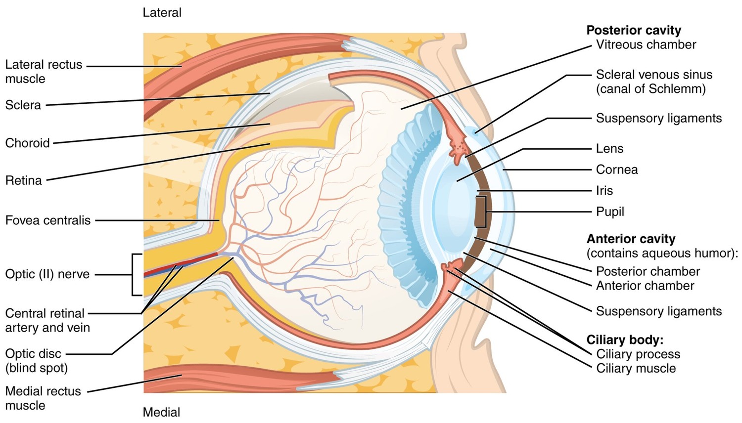
Rods and cones supply most of the signals used for image-forming vision. Rods support vision at low light levels; because they share one spectral sensitivity, rods alone cannot distinguish wavelength from intensity. Cones support daylight color vision through three receptor classes. At intermediate levels, rods and cones both contribute. Their distribution is nonuniform: cones are densest near the center of gaze, while the central foveola lacks rods (Figure 3.1.2). Looking slightly away from a faint star can therefore make it easier to detect.
Foveal cones are only a few micrometers across, with spacing near $2.5\,\mu\text{m}$ in a dense central mosaic; sizes and spacing vary across observers and retinal position. Away from the fovea the cones grow to several micrometers and thin out, while rods, about $1$ to $2\,\mu\text{m}$ across, fill the spaces between them; in Curcio and colleagues' measurements, cone density peaks near 200,000 per square millimeter at the foveal center and rod density near 150,000 per square millimeter about twenty degrees out Curcio et al. 1990. Dense sampling supports fine detail, but does not alone determine acuity. Optical blur, neural pooling, contrast, and illumination also matter. A camera photosite and a cone of similar size need not have similar sensitivity or angular resolution.
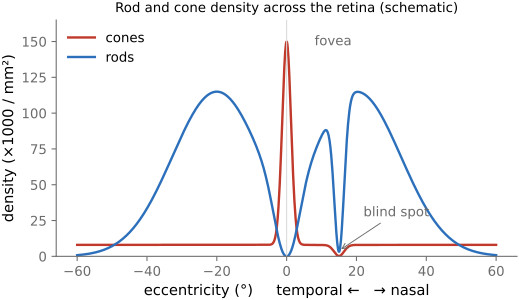
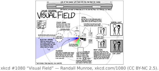
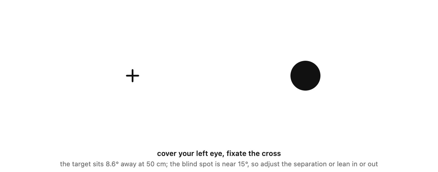
The gap at the optic disc is worth more than a label, because it is the first and cleanest evidence that what you see is constructed. Each eye has a patch of its visual field about five degrees across, some fifteen degrees to the ear side of where you are looking, that delivers nothing at all, and you have never once noticed a hole there. Two things hide it. The other eye covers that part of the field, so closing one is enough to remove the first explanation. What remains is the second and the interesting one: the missing region is filled in with whatever surrounds it, so a line broken exactly there is seen as continuous and a textured field closes over the gap. Nothing in the retina reports the fill; it is manufactured, and it is indistinguishable from the real thing (Figure 3.1.4).
S cones are sparse and absent from a small region at the very center of the fovea. Short-wavelength detail also suffers from the eye's chromatic aberration. Fine luminance detail is carried mainly by combined L- and M-cone signals, while purely chromatic variations have lower spatial resolution. This does not make a green channel identical to luminance, or imply that blue detail is universally sharp through filling-in. The relative importance of luminance detail helps motivate the extra green samples in the Bayer pattern (Chapter 4.6, Sensing color: multiplexing strategies).
The retina processes signals before sending them along the optic nerve. Photoreceptors connect through intermediate neurons to ganglion cells. Many ganglion cells compare a central region with its surround, making them sensitive to local contrast; others have different spatial, temporal, or chromatic selectivity. Signals then reach several brain regions, including the lateral geniculate nucleus and visual cortex. A camera-to-retina analogy is useful for the optics, but retinal output is already a collection of processed signals.
Focus errors provide another connection to camera optics. In a simplified eye, myopia places the image of a distant point in front of the retina; hyperopia places it behind the retina when accommodation is relaxed. Astigmatism gives different focusing power along different orientations. Presbyopia reduces the range over which accommodation can adjust focus with age. These are different optical problems, not one generic blur.
Lens power is expressed in diopters:
where $f$ is the signed focal length in meters. A converging lens with focal length $0.5$ m has power $+2$ diopters; a diverging lens of $-0.5$ m has power $-2$ diopters. This describes the lens, not a complete eye prescription: cylinder power and orientation also matter for astigmatism.
An autorefractor estimates refractive error from light returned by the eye; subjective comparison with trial lenses refines the result. A Shack–Hartmann sensor measures the slopes of the outgoing wavefront using a lenslet array, allowing more detailed aberration estimates. The shared imaging idea is to infer optical properties from the recorded light. Part 22, Compound lenses, and aberration correction develops wavefront measurement.
Perceptual color and trichromatic vision⧉
A display can match the yellow of a flower without emitting the flower's spectrum. Different physical lights can produce the same visual response. That makes color reproduction possible, but also means that a color match tells us little about the underlying spectrum.
We distinguish the light's spectrum, the cone responses it produces, and its appearance in a particular context. Color matching is a measurable relation between stimuli for an observer under specified conditions. A standard observer summarizes such measurements; it does not eliminate variation between people or predict every aspect of appearance.
Cone photoreceptors and perceptual color⧉
Even though cones are known to be the color vision receptors, a single cone does not measure wavelength; it produces one number, and stimuli of different wavelengths can yield the same response.
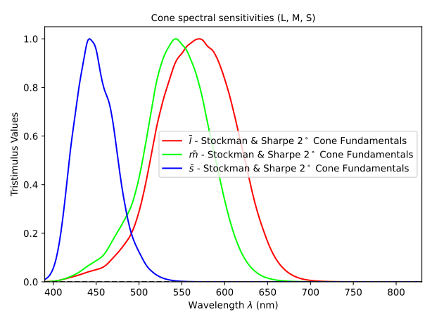
A given cone type $k$ has a spectral sensitivity $c_k(\lambda)$: a curve saying how strongly it responds to light of each wavelength (Figure 3.2.1).
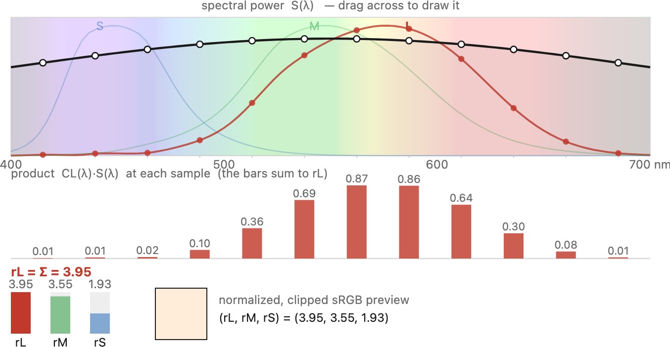
For a fixed state of adaptation, we model the initial cone excitation from an energy spectrum $E(\lambda)$ as a weighted integral, the spectrum weighted by its sensitivity and summed over all wavelengths (Figure 3.2.2):
This linear excitation model precedes the nonlinear adaptation and neural response. Use energy-based sensitivities with an energy spectrum, or quantum-based sensitivities with photon counts; mixing the two conventions gives a wavelength-dependent error. Mathematically the integral is a continuous dot product. In the case of monochromatic light (a single wavelength $\lambda$) it reduces to the scalar product of the cone's sensitivity at $\lambda$ and the light's intensity for $\lambda$.
As Figure 3.2.3 shows, lights at different wavelengths can yield the same response if their intensity ratio is the inverse of the cone's spectral response ratio for those two wavelengths. A single cone conflates wavelength with intensity, a property called univariance.
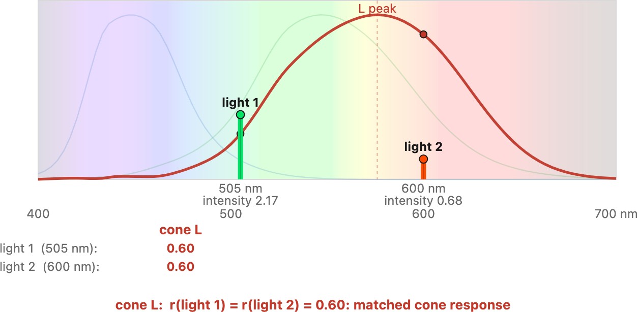
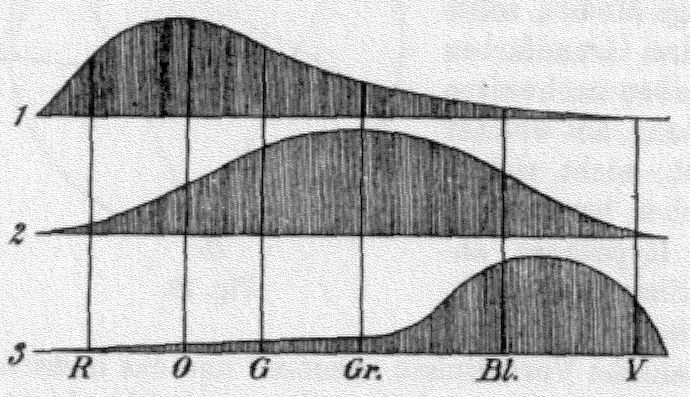
While a single cone cannot distinguish wavelength, the combination of three cone responses provides much more information (click on "show other cones" in Figure 3.2.3 ). This is the trichromatic theory of color vision, pioneered by Thomas Young and put on a quantitative footing by Hermann von Helmholtz.
For photopic color matching, a fixed observer is modeled by three cone excitations $(r_L,r_M,r_S)$. Equal excitations predict a match when spatial, temporal, and adaptation conditions are held fixed. Rod contributions, receptor differences between observers, and contextual appearance require additional considerations.
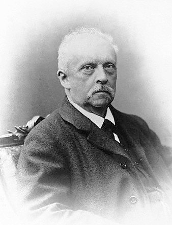 Hermann von Helmholtz (1821–1894) was the physicist and physiologist who turned Thomas Young's guess into a working theory. Young had argued decades earlier that the eye cannot possibly carry a separate detector for every wavelength and must instead make do with a few receptor types; Helmholtz developed this quantitatively, and the three-receptor account of color vision is still called the Young–Helmholtz theory. His Handbook of Physiological Optics founded the field, and he invented the ophthalmoscope that let physicians look into the living eye. Two of his ideas run straight through this chapter. The first is trichromacy itself, the L/M/S projection that everything here is built on. The second is unconscious inference, his claim that perception is not a direct readout of the retina but an inference the brain makes about the most likely cause of its input. That is exactly the stance we take later on color constancy, white balance, and "the dress," where the visual system guesses the illuminant and quietly discounts it. Beyond vision he is everywhere in physics as well, from the conservation of energy to the Helmholtz free energy and the acoustic resonators that carry his name. Portrait: 19th-century photograph, public domain (via Wikimedia Commons).
To compute the integral, sample an energy spectrum at wavelengths $\lambda_i$ with bin widths $\Delta\lambda_i$. Put the spectral-density values into $\mathbf E$, and define the matrix entries as $C_{ki}=c_k(\lambda_i)\Delta\lambda_i$. Then
Each term is the excitation contributed by one wavelength bin. The bin width matters: doubling the number of samples should improve the approximation, not double the response. With nonuniform samples, use the appropriate quadrature weights. Figure 3.2.5 illustrates the matrix computation.
response = [0, 0, 0]
for each wavelength bin i:
    for each cone type k:
        response[k] += spectrum[i] * sensitivity[k, i] * bin_width[i]
Keep spectrum and sensitivity on the same wavelength grid and use one wavelength unit throughout.
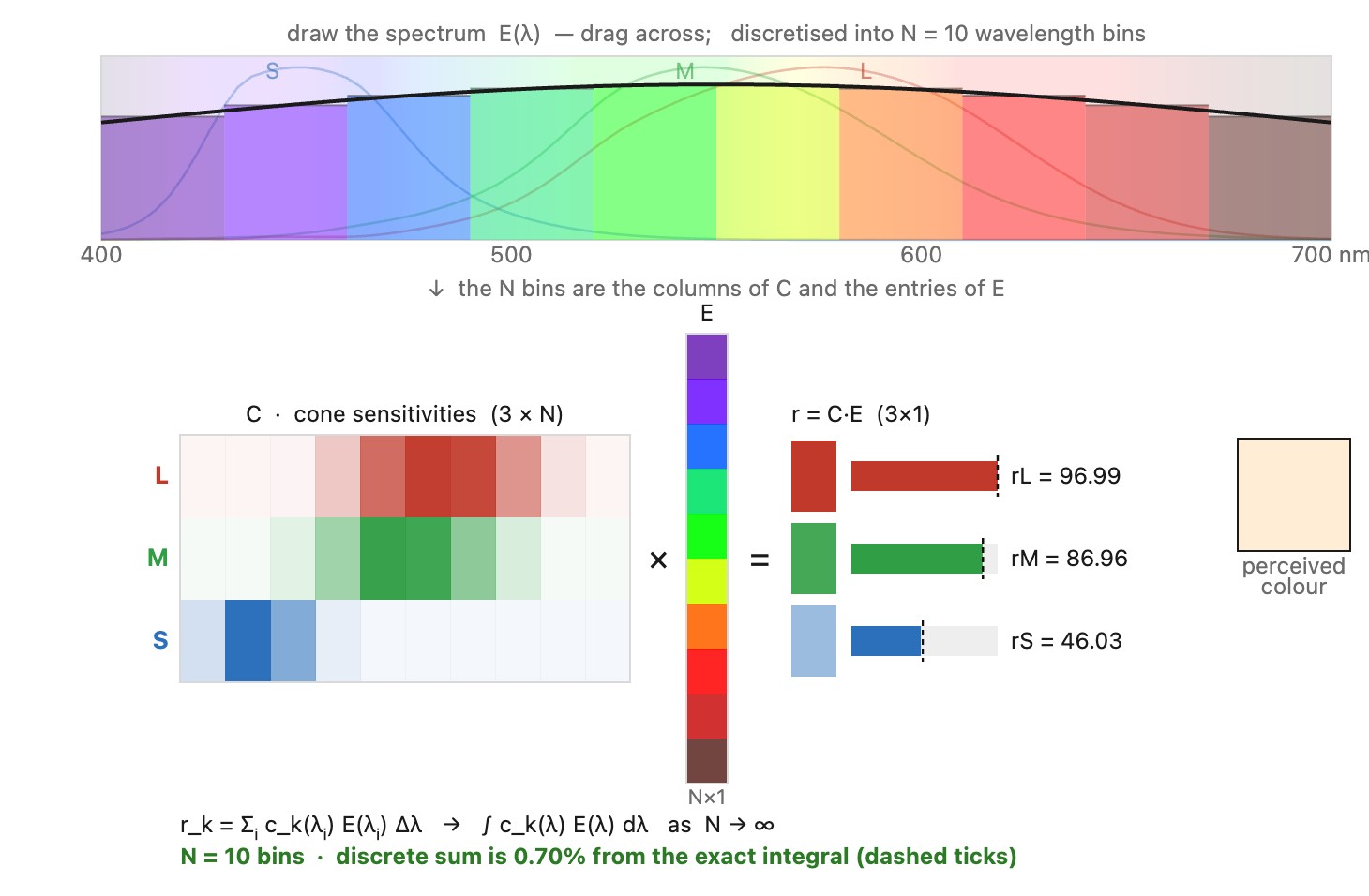
Each cone excitation is an integral of spectral density times the appropriate sensitivity. A sampled implementation must include wavelength-bin widths (or absorb them into the matrix). Three excitations summarize photopic color matching for a fixed observer and viewing condition; they do not recover the spectrum.
We established above that a single cone cannot distinguish wavelengths. Only by comparing the three cones' outputs can the brain begin to separate the two. However, this ability is limited. This is unsurprising because trichromatic vision summarizes a whole spectrum with only three numbers.
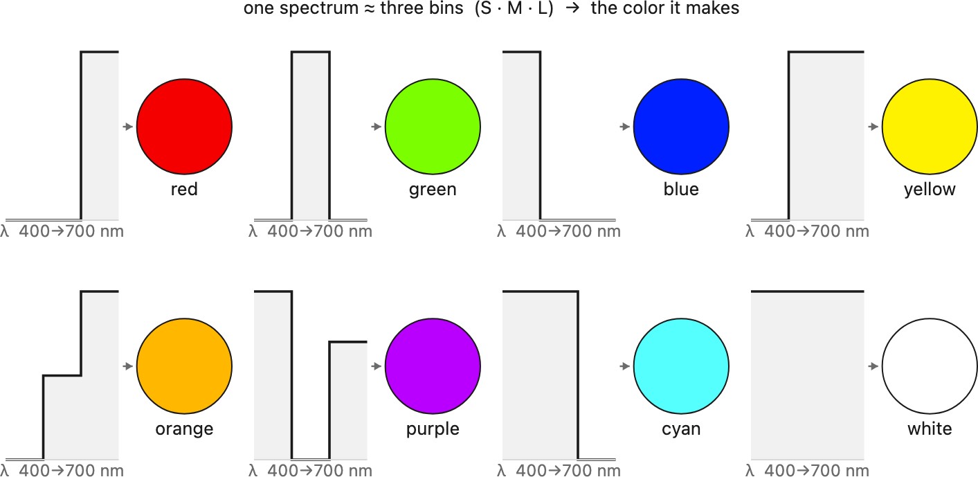
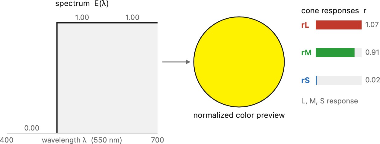
The three-bin examples below are a model of the spectrum, not three isolated cone channels. A bin containing long-wavelength light generally excites both L and M cones. Changing its power changes their ratio as well as their absolute responses. Equal bin powers need not produce equal cone excitations or a neutral white: those depend on the bin boundaries, sensitivity normalization, and reference white. The displayed swatches show an RGB approximation of the resulting color, limited by the screen's gamut.
A few cases make the three-number code concrete. Put the power in the long-wavelength bin and L responds most, M somewhat less, S hardly at all: red. Put it in the short bin and S leads: blue. In the middle bin, M leads with L close behind: green. Fill the long and middle bins together, with little short, and L and M both respond strongly, with L further ahead than for the middle bin alone: yellow, a color with no bin of its own, which is the sign that yellow sits next to green in cone space. All three bins at comparable power give a color near white, depending on the normalization. Orange (mostly long, some middle), cyan (middle plus short) and purple (long plus short, skipping the middle) fill in the hue circle. Every named color is a ratio of three cone catches, and very different spectra can land on the same ratio.
Metamers⧉
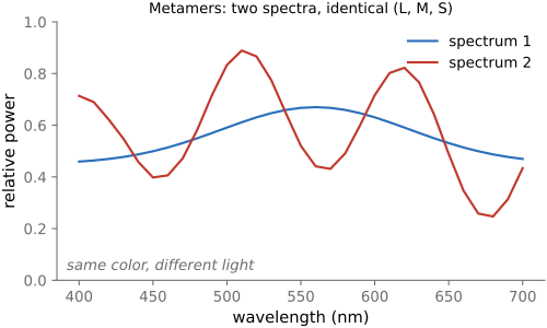
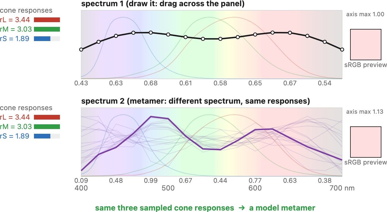
Different nonnegative spectra can produce the same cone-response triple. Such spectra are metamers for that observer and viewing condition. In the sampled model, a spectral perturbation in the null space of $\mathbf C$ leaves the responses unchanged, provided the modified spectrum remains nonnegative (Figure 3.2.8). Displays exploit this: they reproduce an in-gamut color by emitting a metamer rather than the original spectrum. Three fixed physical primaries cannot reproduce every visible color (Chapter 4.1, Linear color reproduction and CIE XYZ).
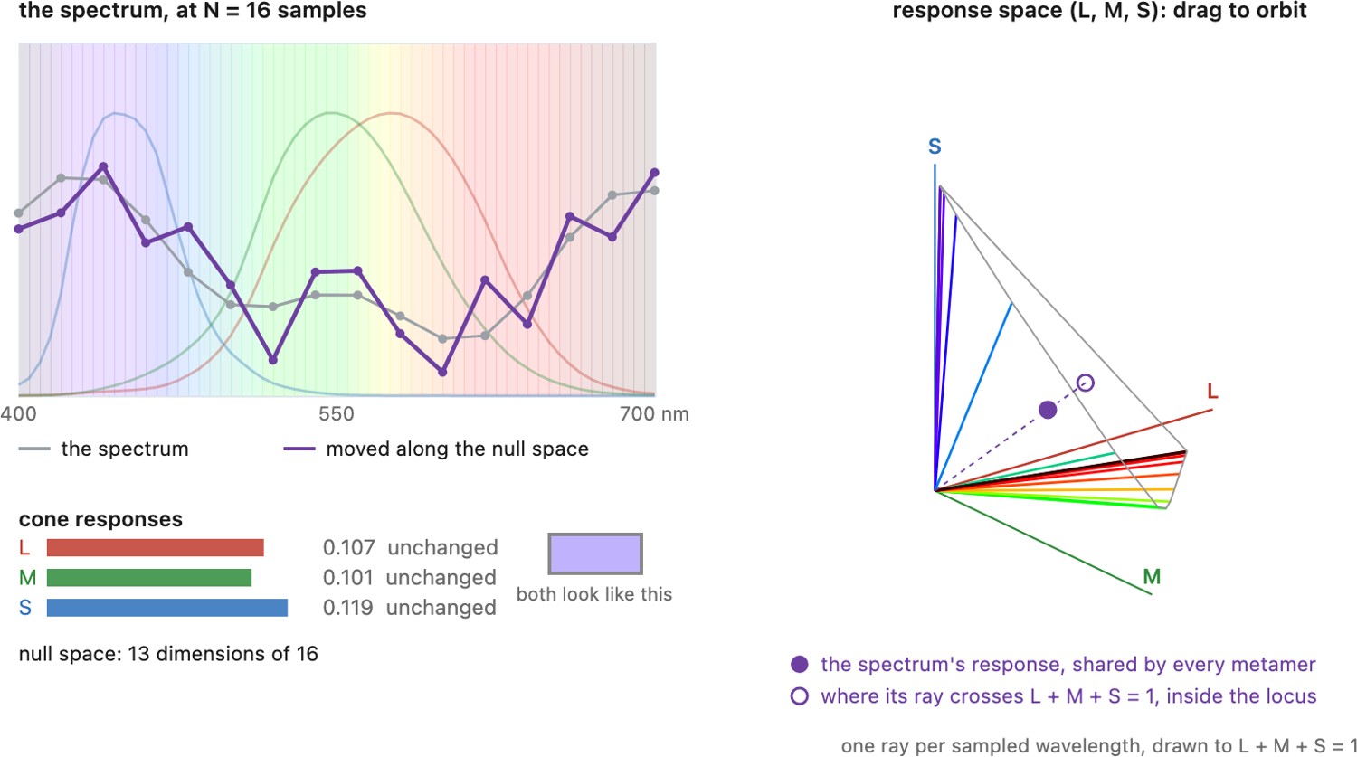
Different spectra can yield the same cone excitations for a specified observer. This enables color reproduction without reproducing the spectrum, but a fixed display can match only colors within its gamut. Matches between reflecting materials can fail when the illuminant changes.
Overlapping cone sensitivities limit the response combinations obtainable by changing a spatially uniform spectrum. Fong, Doyle, Wang and colleagues used adaptive optics, cone classification, and eye tracking to direct light preferentially to selected cone types Fong et al. 2025 (Oz / "olo") Roorda & Williams 1999. Observers reported a highly saturated blue-green, named “olo,” outside the gamut of conventional spatially uniform spectral stimulation. The system changes where light lands on the receptor mosaic; it still uses light. A conventional display cannot reproduce that experience. See Chapter 37.6, Retinal projection.
Dolby 3D uses separate spectral bands to deliver different images to the two eyes. Each eye receives its own red, green, and blue primary bands through matching filters Jorke & Fritz 2003 (Infitec / Dolby 3D). Color correction seeks to match the two eyes' rendered colors within the gamuts the primary sets share. The individual red bands need not be metamers by themselves: the match uses mixtures of each set of primaries. Filter leakage, viewing angle, and observer differences limit the separation and color match.
Two fabrics can match in a shop and differ outdoors. For a nonfluorescent surface in the simple reflectance model, the spectrum reaching the eye is proportional to illuminant times reflectance. A change of illuminant weights the reflectance differences differently, so equality of the three integrals need not survive (Figure 3.2.13). Narrow spectral peaks can make matches sensitive to particular reflectance differences, but smooth illuminants can also break a match. Color-critical work specifies the illuminant and observer. Figure 3.2.11 shows a printed metameric pair under daylight and halogen illumination.
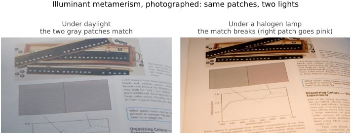
A metameric match is a match between two products of reflectance and illuminant (L2.6). Swap the illuminant and you multiply by a different spectral shape, so two surfaces that looked identical under one light can diverge under another: illuminant metamerism. It is the headache behind prints that shift between the proofing booth and the living room, and fabrics that match in the shop but clash in daylight; color-critical work must always name the light a match is judged under.
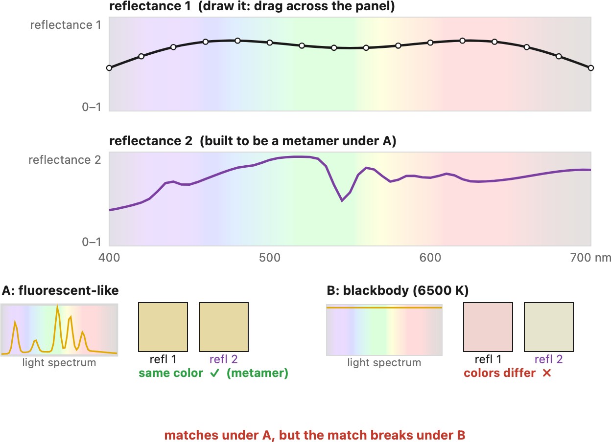
Consider a printer matching a fabric. The inks and the fabric can have quite different reflectance spectra while sending the same three cone responses to an observer under the proofing light. Moving both under another light changes the wavelength-by-wavelength weights before those responses are summed. The differences that canceled under the first light need not cancel under the second. A narrow spectral peak can emphasize a region where the two reflectances differ; a smooth change of illumination can also break the match. This is why specifying only three color coordinates does not promise a match under every illuminant. A proofing agreement needs a viewing illuminant and observer as well as a numerical tolerance.
Color blindness⧉
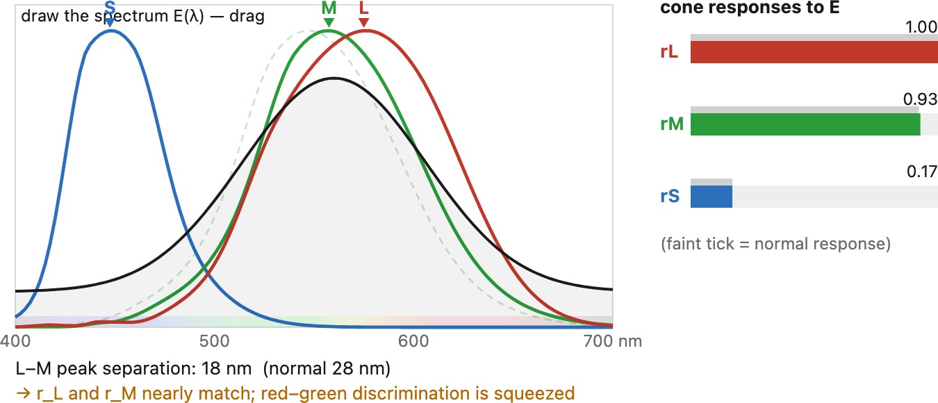
optionalIn dichromatic vision, two functionally distinct cone classes supply the photopic color signal. More spectra then share the same response than for a trichromatic observer. In anomalous trichromacy, three classes remain but their spectral sensitivities differ from the usual model. This can reduce discrimination between particular colors. “Color blindness” covers several conditions; it does not usually mean seeing only gray.
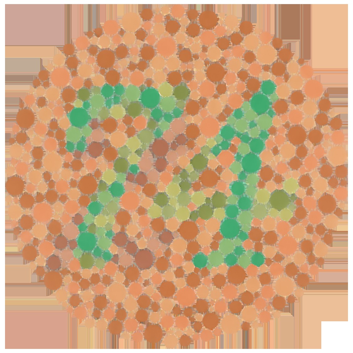
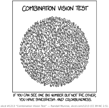
Protan and deutan deficiencies affect the L/M system; tritan deficiencies affect the S-cone system. Complete achromatopsia involves severely impaired cone function and affects acuity and light sensitivity as well as color. Oliver Sacks's The Island of the Colorblind describes its unusually high prevalence on Pingelap Sacks, The Island of the Colorblind. These conditions cannot all be modeled by simply deleting an RGB channel.
Common inherited red–green deficiencies are associated with L/M opsin genes on the X chromosome and occur more frequently in males. Prevalence varies by population. Other deficiencies have different genetic or acquired causes (National Eye Institute).
For imaging interfaces, do not make hue the only way to distinguish information. Use labels, shapes, or adequate lightness contrast as well. Simulations can reveal likely confusions, but they do not reproduce every observer's experience. Screen versions of test plates depend on the display and viewing conditions and should not be treated as a diagnosis. Recoloring and spectral filters can change which differences are visible; they do not add a missing receptor class.
Anyone can check their own color vision in a few minutes. Ishihara plates screen for red-green deficiency; arrangement tests such as the Farnsworth–Munsell 100 hue test, in which the observer orders colored caps around the hue circle, measure discrimination along that circle, and the pattern of errors shows which axis is affected. Online versions are useful screening, with the display caveats above. Help comes in two kinds, neither a cure. Software daltonization remaps an image to push confusable colors apart, and phones and design tools can simulate a deficiency so a designer can check a chart. Notch-filter glasses remove a narrow band where the L and M sensitivities overlap most, which can enlarge the difference between their responses for some anomalous trichromats; they add no pigment and do little for a dichromat.
Both tools start from the same model. To simulate a dichromat, convert each pixel to cone responses and replace them with the closest triple the dichromat's two remaining cone classes cannot tell from it: the response of the missing class is filled in from the other two, so the pixel moves onto a surface in cone space where every color it could be confused with lands on the same point. Brettel, Viénot and Mollon built that surface from two half-planes anchored on colors that dichromats and trichromats describe alike Brettel, Viénot & Mollon 1997; Machado, Oliveira and Fernandes extended the model to anomalous trichromacy by shifting a pigment's sensitivity by a chosen amount rather than removing it Machado, Oliveira & Fernandes 2009. Daltonization then uses the difference between the original and the simulated image, which is exactly the information the viewer loses, and adds it back along a direction the viewer can see, typically into lightness or the blue-yellow axis. Early web tools such as Vischeck made simulation widely available; the same computation now ships in accessibility checkers and in browser developer tools. A simulation predicts which colors collapse, not what the viewer experiences, and daltonization trades the natural look of the colors for their separability.
The genetics explains much of the difference in prevalence. The L- and M-opsin genes are close together on the X chromosome. Recombination between these similar sequences can remove a gene or produce a hybrid pigment gene, changing the set of spectral sensitivities. With only one X chromosome, an affected copy is sufficient for an X-linked deficiency; with two, another functioning copy can protect against it. MedlinePlus Genetics gives about one in twelve males and one in two hundred females for inherited red-green deficiency in populations of Northern European ancestry, with lower frequencies in many other populations. Blue-yellow deficiencies have different inheritance and are much rarer.
| Type | What changes | Males | Females |
|---|---|---|---|
| Protanopia | L cones absent | about 1% | about 0.02% |
| Protanomaly | L pigment shifted | about 1% | about 0.03% |
| Deuteranopia | M cones absent | about 1% | about 0.01% |
| Deuteranomaly | M pigment shifted | about 5% | about 0.4% |
| Tritanopia | S cones absent | about 0.002% | about 0.002% |
| Achromatopsia | little or no cone function | about 0.003% | about 0.003% |
Approximate prevalence in populations of European ancestry, after Sharpe and colleagues Sharpe et al. 1999; red-green rates are lower in many other populations, and published estimates vary with the test used.
This is a useful distinction for the projection model. Anomalous trichromacy changes the measurement curves but retains three functionally distinct classes. Dichromacy reduces their number to two. Monochromacy is a further loss of chromatic discrimination, although different clinical conditions can produce it. A software simulation should model the relevant change in sensitivities, not merely turn off the screen's red or green primary.
Trichromacy itself is also a limitation: three measurements cannot identify an arbitrary spectrum. A trichromat can distinguish some pairs that a dichromat cannot, while both discard most of the spectral information. Calling one observer color deficient should not obscure the same information loss in the standard observer used by imaging systems.
Opponent process and the multistage model⧉
A yellow light need not stimulate a “yellow cone.” Comparisons between cone signals contribute to chromatic processing. Physiological opponent responses and psychophysical hue-cancellation measurements support multistage accounts of color vision De Valois et al. 1966 Hurvich & Jameson 1957. They do not establish that one fixed matrix explains unique hues, afterimages, and color names.
A useful teaching model forms one sum and two differences of the cone signals. For cone contrasts relative to positive background excitations $r_{k,0}$, define
Here $q$ averages the L and M contrasts, $a$ compares them, and $b$ compares S contrast with that average. Equal fractional increases in all three cone excitations change $q$ but leave $a$ and $b$ zero. This is a simplified opponent representation, not a calibrated model of an individual observer's luminance or hue perception.
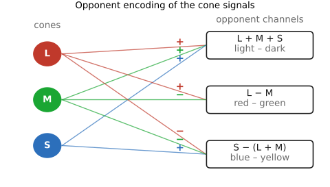
Derrington, Krauskopf, and Lennie studied chromatic mechanisms in macaque lateral geniculate neurons Derrington, Krauskopf & Lennie 1984 (DKL cardinal directions). The resulting DKL framework describes modulations around an adapting background along luminance and chromatic cardinal directions. Its numerical transform depends on cone fundamentals, background, luminance weights, and axis normalization. Our equal-weight matrix illustrates sum-and-difference processing; it should not be substituted for a calibrated DKL transform in an experiment. Cardinal directions also need not coincide with an observer's unique red, green, blue, and yellow.
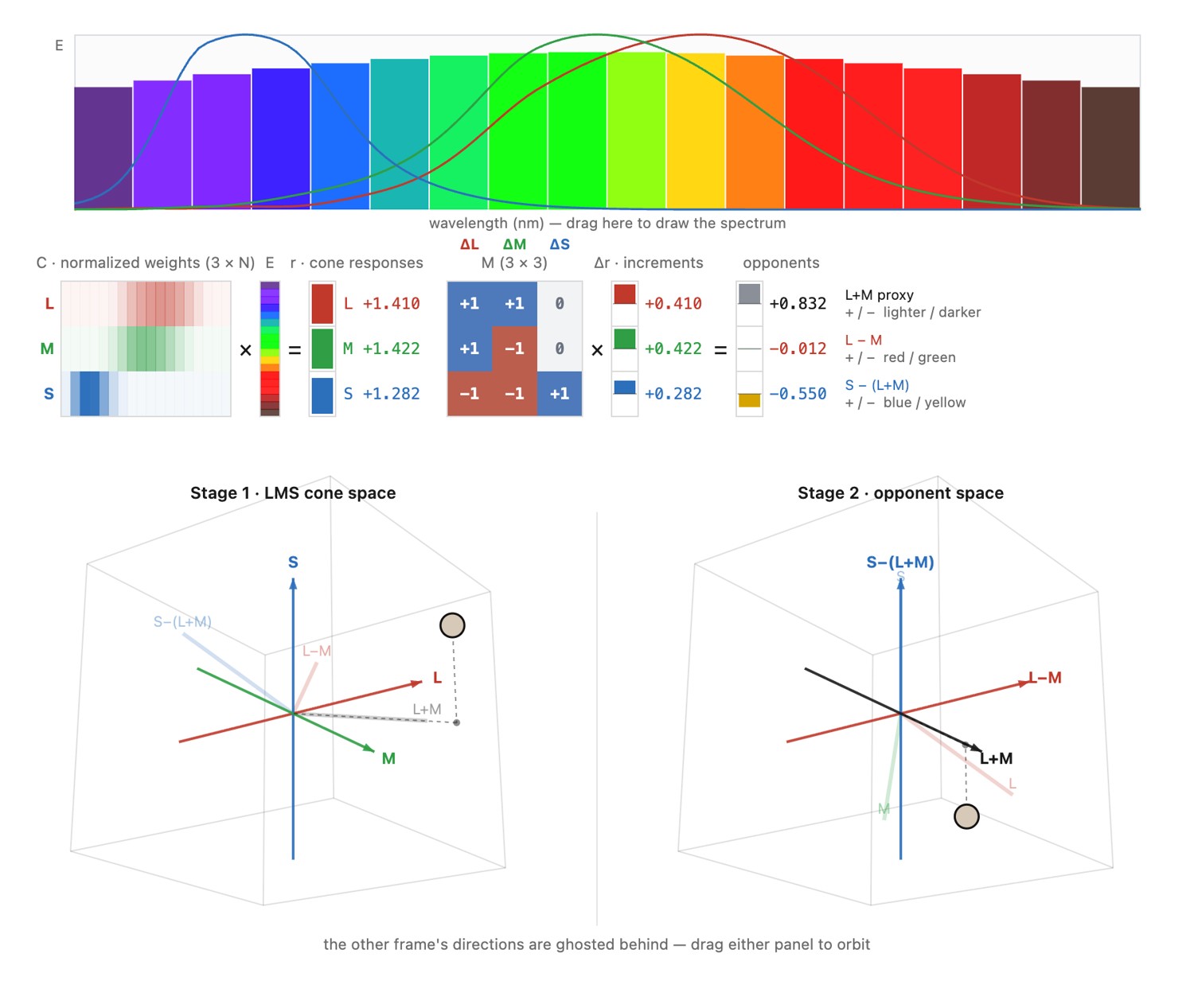
Cone excitations are followed by neural comparisons and adaptation. Sum-and-difference models illustrate this processing, but their axes are not exact perceptual hue axes. Engineering luma/chroma transforms exploit related sensitivity differences without reproducing the neural pathway.
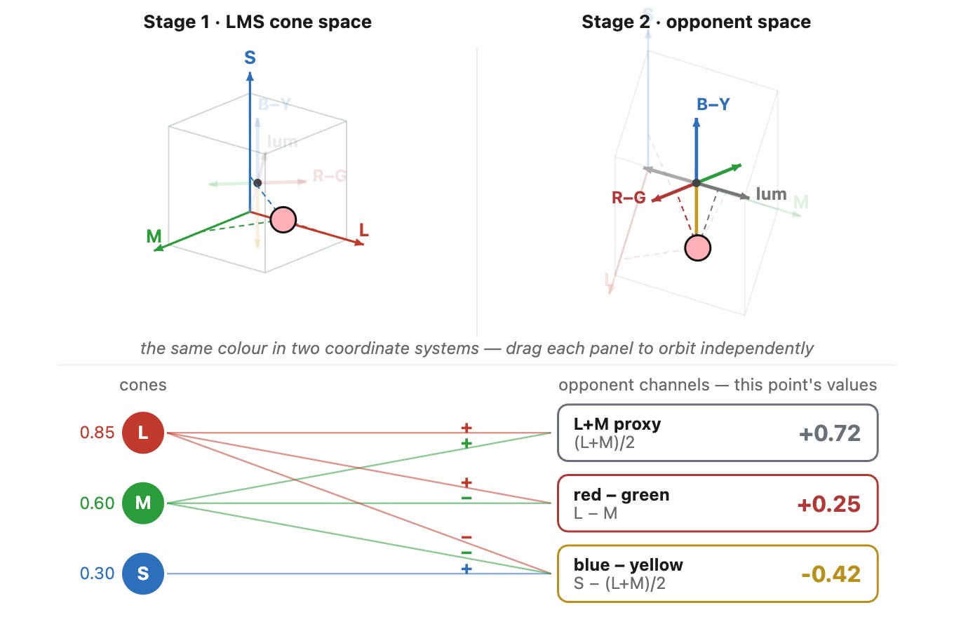
Afterimages involve adaptation across the visual system, including cone and postreceptoral mechanisms (Chapter 3.3, Adaptation and constancy). Compression exploits lower sensitivity to fine chromatic detail, but that is an empirical property of spatial vision, not a consequence of taking differences alone. The engineering channel $Y\prime$ is luma computed from nonlinear RGB, distinct from physical luminance. Thin colored text and saturated edges can reveal chroma-subsampling artifacts.
So what are the primary colors?⧉
optionalA screen adds light from its primaries, usually red, green, and blue. Inks and filters instead modify the spectrum of incident light; cyan, magenta, and yellow are useful subtractive choices. Neither list is a property of light itself. Different primary spectra give different gamuts.
Psychological unique hues describe appearances such as a yellow that seems neither reddish nor greenish. They are not display primaries or cone classes. Traditional red–yellow–blue painting instruction is another use of “primary”; actual pigment mixtures depend on absorption and scattering, and their gamut depends on the pigments chosen. Chapter 4.7, Synthesizing color develops these physical mixing processes.
Specify the purpose when naming primaries: sources whose light is added, inks or filters that absorb light, or perceptual hue judgments. RGB and CMY describe common engineering choices, not unique sets required by nature. The chosen spectra and mixing process determine what can be reproduced.
The ambiguity is why an argument about “the primary colors” so often has no useful answer. A physiologist may mean receptor classes, a painter may mean a set of pigments for mixing, and a display engineer may mean the emitters whose powers can be controlled. A perceptual experiment may instead ask which hues appear unmixed. State which experiment or technology the word refers to before choosing a list. Red-yellow-blue painting instruction is a mixing convention, not a competing account of the cone sensitivities.
Color as linear algebra⧉
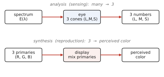
Cone sensing is a linear measurement from many spectral samples to three excitations. It is not an expansion of the spectrum in three basis functions. The sensitivity curves are measurement weights; three of them cannot span an arbitrary spectrum.
Reproduction asks a different question. Put the cone-response triples of three chosen primary lights in the columns of a $3\times3$ matrix $\mathbf A$. To match target responses $\mathbf r$, solve
The entries of $\mathbf p$ are primary powers. Even if $\mathbf A$ is invertible, a negative entry means the target cannot be emitted by adding those primaries. A finite display also imposes upper limits. This separates two issues: solving a linear system and producing its solution with physical light. Chapter 4.1, Linear color reproduction and CIE XYZ develops the distinction.
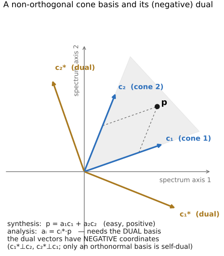
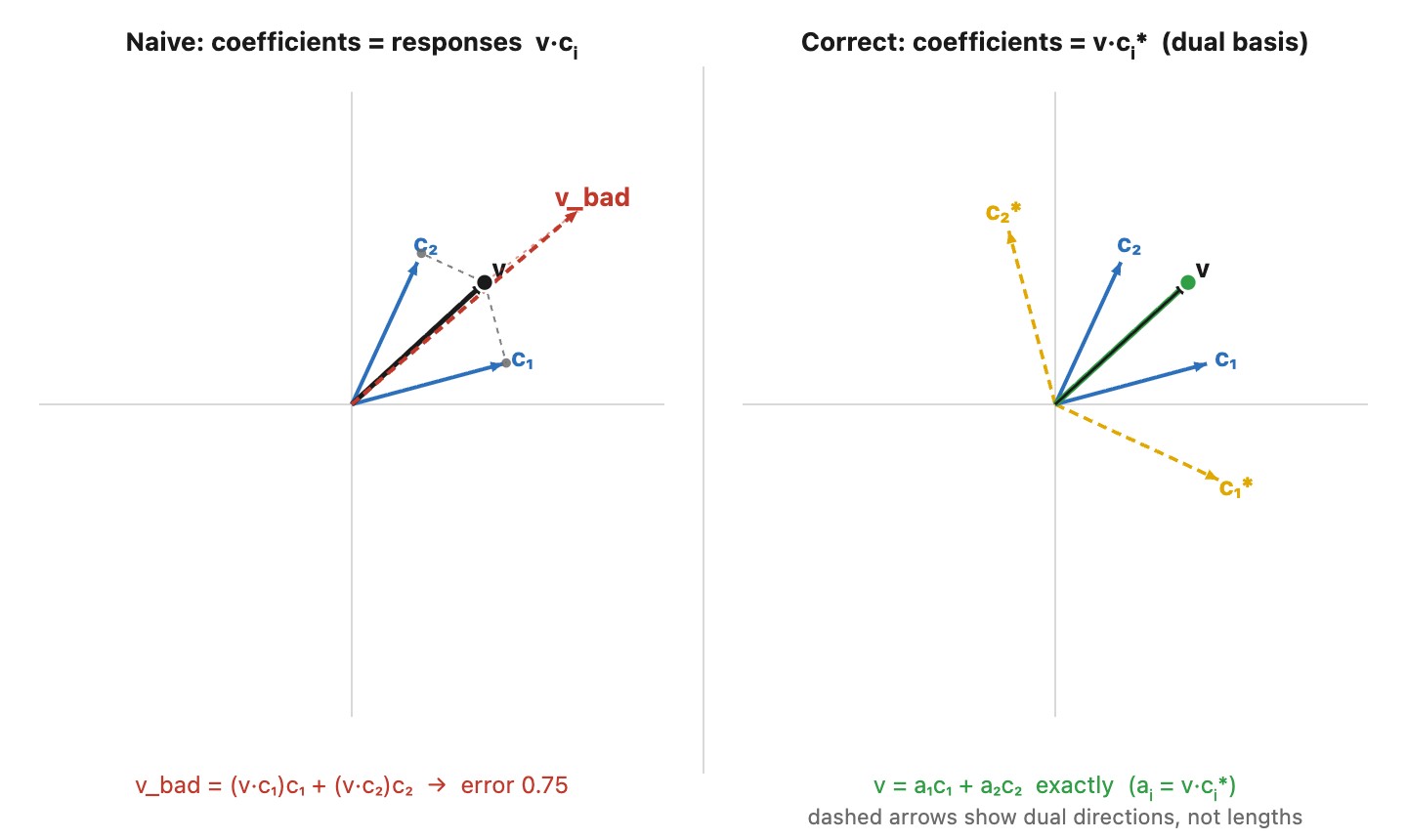
A two-dimensional basis-and-dual diagram (Figure 3.2.20) illustrates why dotting with nonorthogonal synthesis vectors does not directly recover their coefficients. It is a linear-algebra analogy, not a model in which cone curves form a basis for all spectra.
Cone sensitivity curves overlap, and physical spectra and emitted primary powers are nonnegative. Cone responses are measurements, not spectrum coefficients. Matching a response triple with three primary lights requires solving for their powers; a negative solution identifies a color outside those primaries' additive gamut.
The overlap of the sensitivity curves and the nonnegativity of light are separate constraints. Because L and M sensitivities overlap strongly, an ordinary spectral change usually affects both responses. We cannot freely prescribe one response while holding the others at zero simply because three coordinates are available on paper. A mathematical solution can call for subtracting light at some wavelengths; a physical source can only supply a nonnegative spectrum. This is the connection between the cone-sensitivity plot and the gamut restrictions on the reproduction solve.
Linear color reproduction and CIE XYZ⧉
A color match reproduces an observer’s responses to light without reproducing its spectrum. For a fixed standard observer, tristimulus coordinates describe these matches with three numbers. The central calculation is linear, but its physical constraints matter: a display can add light from its primaries, not subtract it.
The color reproduction perspective⧉
optionalIn principle, measuring color and reproducing it are separate problems. Given light, measurement reports coordinates for its color. Given those coordinates, reproduction builds light on a screen or a page that matches it. You could imagine a camera reporting device-independent measurements to a separate display module, with neither module needing to know how the other works. Much of the notation we actually use comes from treating them together as a reproduction pipeline.
The reason is historical and experimental. Color matching provided a way to measure perceptual color before cone sensitivities could be measured directly. An observer adjusted three fixed primary lights until their mixture matched a test light. The three knob settings were the measurement. These coordinates therefore described amounts of particular reproduction primaries, rather than direct cone responses. Changing the primary lights changed the coordinates of the very same test light. The experiment made measurement possible, but also made the reproduction apparatus part of the measurement convention. Television reinforced the practical importance of a primary-based description: a central engineering task was to get the right picture out of a particular screen.
Metamerism makes this useful. Different spectra can match for the specified observer and conditions. They may cease to match for another observer, or after a change of illumination when the spectra come from reflecting objects. Colorimetry describes the match; it does not by itself predict appearance across different surrounds and adaptation states.
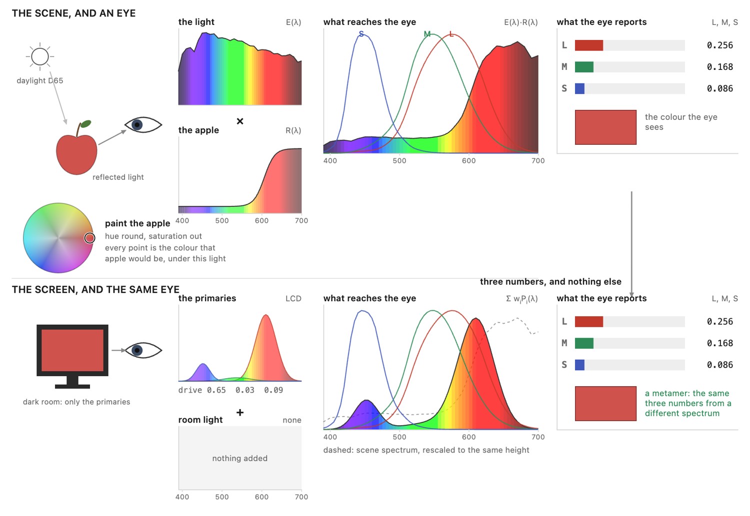
XYZ provides a common reference for device characterization and color conversion. The agreement matters as much as the matrix algebra. With a shared reference, a new display can describe its primaries once instead of requiring a separately standardized conversion from every existing camera or working space. Conversion between two linear tristimulus coordinate systems for the same observer is a matrix multiplication. The shared reference lets those conversions be composed. A camera’s three raw channels generally do not span exactly the standard observer’s matching functions, so its color-correction matrix is an approximation fitted to a calibration set. Nonlinear encodings must be decoded before applying linear-light color matrices.
Changing illumination is another limitation. The illumination multiplies reflectance wavelength by wavelength, whereas a three-channel measurement has already discarded most of that spectral information. A three-by-three chromatic-adaptation transform is a useful model of corresponding colors, not a general solution to spectral relighting. Smooth illumination alone does not make it exact.
A typical rendered-image path includes black-level correction, white-balance gains, demosaicking, camera color correction, tone and color rendering, and output encoding. Implementations combine or reorder some stages. XYZ often enters through the calibration that defines the matrices rather than as a separately stored image. To convert between two linear RGB systems, we can compose an RGB-to-XYZ matrix with an XYZ-to-RGB matrix and apply the resulting matrix directly. The intermediate XYZ coordinates define the conversion without needing to be written into an image buffer. This is why XYZ can be central to a system whose working images are all called RGB.
Analysis vs synthesis and non-orthogonality⧉
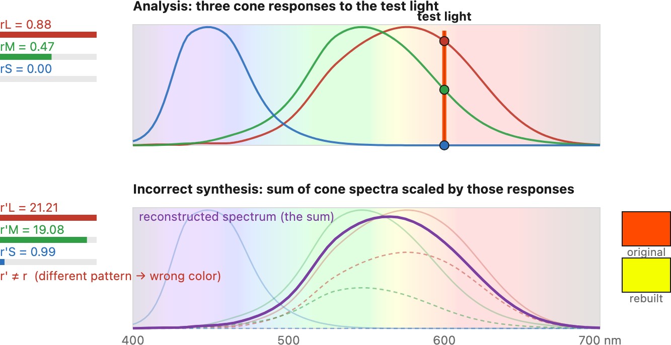
First imagine three nonoverlapping, flat sensitivity bands. Measuring the power in each band and emitting the same power within that band would reproduce the three measurements. Human cone sensitivities overlap instead: a light chosen to stimulate one cone type also stimulates others. If we use the sensitivity curves themselves as emission spectra, then scale them by the measured responses, measuring the result applies that overlap a second time. The responses generally change, as Figure 4.1.3 shows. We need to account for how every chosen primary stimulates every analysis channel.
The failing construction is short enough to write out. Emit the sensitivity curves weighted by the responses, $\hat{\mathbf e}=C^{\mathsf T}\mathbf r$, and measure the result: the responses come back as $C\hat{\mathbf e}=CC^{\mathsf T}\mathbf r$. The three-by-three matrix $G=CC^{\mathsf T}$ holds the overlap of every pair of curves, and it is the identity only if the curves are orthonormal. For cones it is far from that, above all for L and M, which overlap heavily, so a light that should excite mostly L comes back measured as a large L and M mixture, and a monochromatic test light is rebuilt as a broad, desaturated one (Figure 4.1.3). The correct weights are $G^{-1}\mathbf r$, which is what the dual basis computes, and they include negative entries: to reproduce the test light with these curves as emitters we would have to subtract light, which is the same wall that real primaries hit in the next section.
Sample an incoming spectrum into a vector $\mathbf e$. Let $C$ be a three-by-$N$ analysis matrix, including wavelength-bin weights, and let the columns of $P$ be three sampled display-primary spectra. Measurement and reproduction are
Thus matching the target requires solving $A\mathbf p=\mathbf r$, where $A=CP$. Each column of $A$ gives the three measured responses to one display primary. If $A$ is invertible, there is a unique algebraic solution. The display can realize it only if every primary weight lies within its allowed range.
Sensitivity curves measure a spectrum; emission primaries construct one. Reusing the sensitivity curves as primaries and the measured responses as weights generally gives the wrong color. Calibrate how each primary stimulates the observer, then solve for its weight.
The problem color reproduction actually solves is not quite the textbook one. In linear algebra, reconstruction means rebuilding a vector exactly as a linear combination of basis vectors, so that the result equals the original. Color reproduction asks for less. We do not need the reproduced spectrum to equal the original spectrum, only to produce the same three cone responses, that is, to be a metamer of it. That is a weaker requirement, a match of projections rather than of whole vectors, and it buys a great deal of freedom: the reproduction primaries can be chosen independently of the analysis (cone) vectors, they can be picked to be physically realizable lights, and an in-gamut color can still be matched. Solving the primary-response system gives the coefficients for a given set of primaries; metamerism is what lets us choose those primaries in the first place.
This is where the usual non-orthogonal-basis intuition helps, provided we apply it to the right space. The three primary-response columns need not point along independent cone axes. Solving their linear system compensates for the cross-talk. Merely using a measured cone response as the weight of a similarly shaped emitter applies the cross-talk again. The distinction between taking dot products and solving for synthesis coefficients is familiar from dual bases in linear algebra; here the goal is equality of three measurements, with no requirement to reconstruct the original spectrum.
The algebraic solution can include a negative primary weight. That is a useful coordinate, but a display cannot emit negative light to subtract the unwanted response of another primary. Its physically available mixtures form a restricted set. Metamerism gives us freedom to use a different spectrum for a match; it does not ensure that a particular display's positive mixtures contain a match for every visible color.
The representation labels are a practical type system. A matrix accepting linear RGB cannot be applied directly to encoded RGB merely because both have three components. A luminance and a luma can both be called brightness in conversation while requiring different computations. Before composing two matrices, check that the first one's output has the second one's expected primaries, reference white, normalization, and encoding. The matrix dimensions alone cannot catch these mistakes. This is why color code needs more bookkeeping than an arbitrary three-vector calculation.
Label the representation at each transition. In this part, bare RGB denotes linear values, primes denote a specified nonlinear encoding, and a superscript $\ell$ denotes a specified log encoding. The curve must still be named: a prime does not distinguish sRGB, Rec. 709, or PQ. PQ can encode RGB as well as coordinates used inside ICtCp. A matrix signature states its input and output, for example $M:\mathrm{RGB}_{709}\to\mathrm{XYZ}$. Equal input and output types do not imply an identity operation; exposure scaling is an obvious counterexample.
Color matching and the most standard color space: CIE XYZ⧉
Why measure color through matching experiments rather than directly through cone responses? When the CIE established its 1931 standard, direct measurements of human cone spectral sensitivities were not available. Observers could nevertheless tell when two lights matched. That gave colorimetry an experimental route: define the analysis of a light by measuring its synthesis from adjustable primaries. Metamerism makes this possible because the spectra need not be identical, and the additivity of matches lets the measured coordinates be used for mixtures.
The design of that experiment is why it worked. Psychophysics, putting a number on a private sensation, is slippery: observers disagree, adapt, tire, and shift their answers with the surround and the wording of the task. A matching experiment asks for none of that. It is a null measurement: the observer reports only when the two halves of a field look the same, which people do far more reliably than they rate how different two colors are. Metamerism keeps the answer to three numbers rather than a spectrum, and linearity lets a limited set of measured matches extend to every mixture. The 1931 standard rests on the matching data of Wright and of Guild, about seventeen observers across the two studies, and it still predicts matches for typical observers well enough to anchor color measurement nearly a century later, within the limits of an average observer that the rest of this chapter keeps in view.
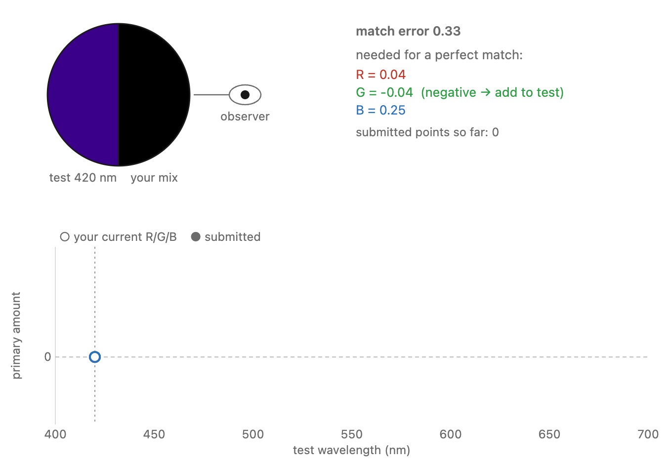
In a color-matching experiment, an observer views a test light beside a mixture of three fixed primaries. The primary amounts required for a match define its tristimulus coordinates. Some stimuli cannot be matched with nonnegative amounts: adding a primary to the test side is recorded as a negative amount on the mixture side. Repeating the experiment across wavelength gives the matching functions for those primaries. Wright and Guild used different primaries, and the CIE converted both data sets to three common monochromatic primaries at 700 nm, 546.1 nm and 435.8 nm Fairman, Brill & Hemmendinger 1997. The last two are emission lines of mercury, which any laboratory could reproduce exactly. The red was placed at 700 nm because in that part of the spectrum the hue hardly changes with wavelength, so a small error in setting it hardly changes the match. Spreading the three primaries far apart also keeps them well separated in cone response, the red and green especially, so the matching system is well conditioned.
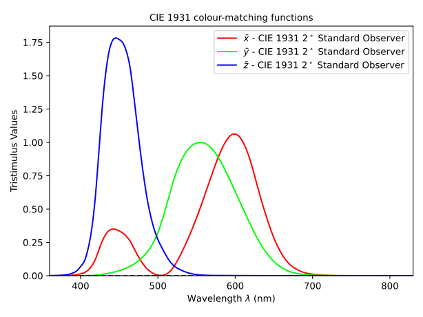
The CIE 1931 standard transforms the measured matching functions to imaginary XYZ primaries. These are coordinate axes, not three lamps. The transformation makes all three XYZ matching functions nonnegative and makes $\bar y(\lambda)$ equal to the standard photopic luminous-efficiency function. For a spectral stimulus $E(\lambda)$,
The normalization $k$ determines the scale. For relative tristimulus values, choose it so the reference white has $Y=1$ (or explicitly $100$). For spectral radiance in physical units, the photometric conversion gives $Y$ in cd/m², with a factor approximately 683 lm/W and consistent wavelength units. Relative $Y=1$ is not one cd/m². Neither version of luminance is a full prediction of perceived brightness.
For sampled spectra, include bin widths:
XYZ = [0, 0, 0]
for each wavelength bin i:
    XYZ += k * E[i] * [xbar[i], ybar[i], zbar[i]] * delta_lambda[i]
Use tables for the intended observer and field size. The CIE 1931 two-degree tables specify one standard observer, not every individual’s cone sensitivities.
LMS coordinates can be defined as a linear transform of XYZ for a chosen colorimetric observer. That does not make modern physiological cone fundamentals an exact transform of the older 1931 observer. For example, the Hunt–Pointer–Estévez transform used in appearance models is
These model coordinates should not be substituted silently for measured cone excitations or a different normalization of cone fundamentals.
XYZ, a compatible LMS system, and linear RGB are different coordinates for a fixed observer’s three-dimensional color matches. Nonlinear RGB encodings and perceptual spaces add specified nonlinear transforms. A real camera’s raw measurements usually require an approximate color correction; an appearance model also needs viewing conditions.
A reference chart used in color characterization. Its patches sample a useful set of surface colors but do not prove accurate reproduction of every spectrum. See Chapter 45.16, Datasets.
The negative-primary case is easiest to understand at the apparatus. Suppose a saturated test cannot be matched by adding any nonnegative mixture of the three primary lamps. Move some red primary light to the test side, then adjust green and blue on the matching side until the fields agree. The recorded red coefficient of the original test is negative because that red was added to the opposite side of the equality. No lamp emits negative light. Linearity lets us subtract its contribution algebraically.
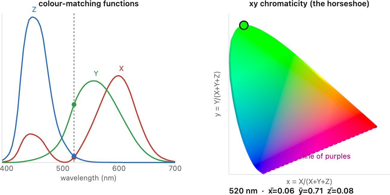
Repeat the match with narrow-band test lights across wavelength. The three settings at each wavelength form the color-matching functions. A broad spectrum can then be treated as a sum of these narrow-band contributions, which is why the integral above predicts its tristimulus coordinates. Transforming those coordinates to XYZ changes the coordinate system; it does not require building three imaginary lamps. A monitor illustration can show the controls and equations, but its own primaries limit which test spectra and matches it can physically reproduce.
One might wish that color technology had started with LMS: its axes have a direct interpretation in terms of the receptors. Later measurements of cone photopigments and the development of cone fundamentals made that interpretation much more accessible [@bowmaker-dartnall-1980; @stockman-sharpe-2000]. By then XYZ was already embedded in instruments, specifications, and device characterization. Replacing the common reference would have imposed a compatibility cost on all of them. XYZ also supplies a convenient luminance coordinate and nonnegative matching functions. Its persistence is therefore understandable even though its imaginary primaries and experimental origins make it harder to explain.
Keep the historical argument separate from the observer model. Linear coordinate changes preserve the matches of a fixed observer. A later physiological observer can differ from the 1931 standard; adopting it is not merely renaming the older coordinates. We can explain why XYZ stayed in use without claiming that every modern cone fundamental is an exact transform of the 1931 tables.
Chromaticity diagram⧉
For $X+Y+Z>0$, define
These coordinates discard scale: doubling the light leaves $x,y$ unchanged. Black has undefined chromaticity. Given $xyY$ with $y>0$, recover $X=xY/y$ and $Z=(1-x-y)Y/y$. Thus chromaticity plus luminance specifies the original tristimulus values; chromaticity alone does not.
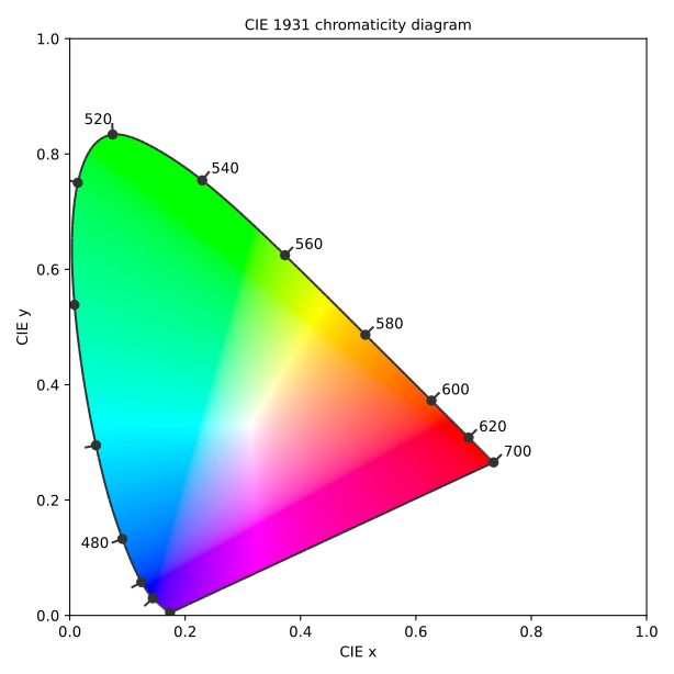
Monochromatic lights trace the spectral locus. Nonnegative mixtures lie in its convex hull, closed by the line of purples. The reference white is a selected point within this region, not an intrinsic center of the diagram. Euclidean distance in $xy$ is not a perceptual color difference.
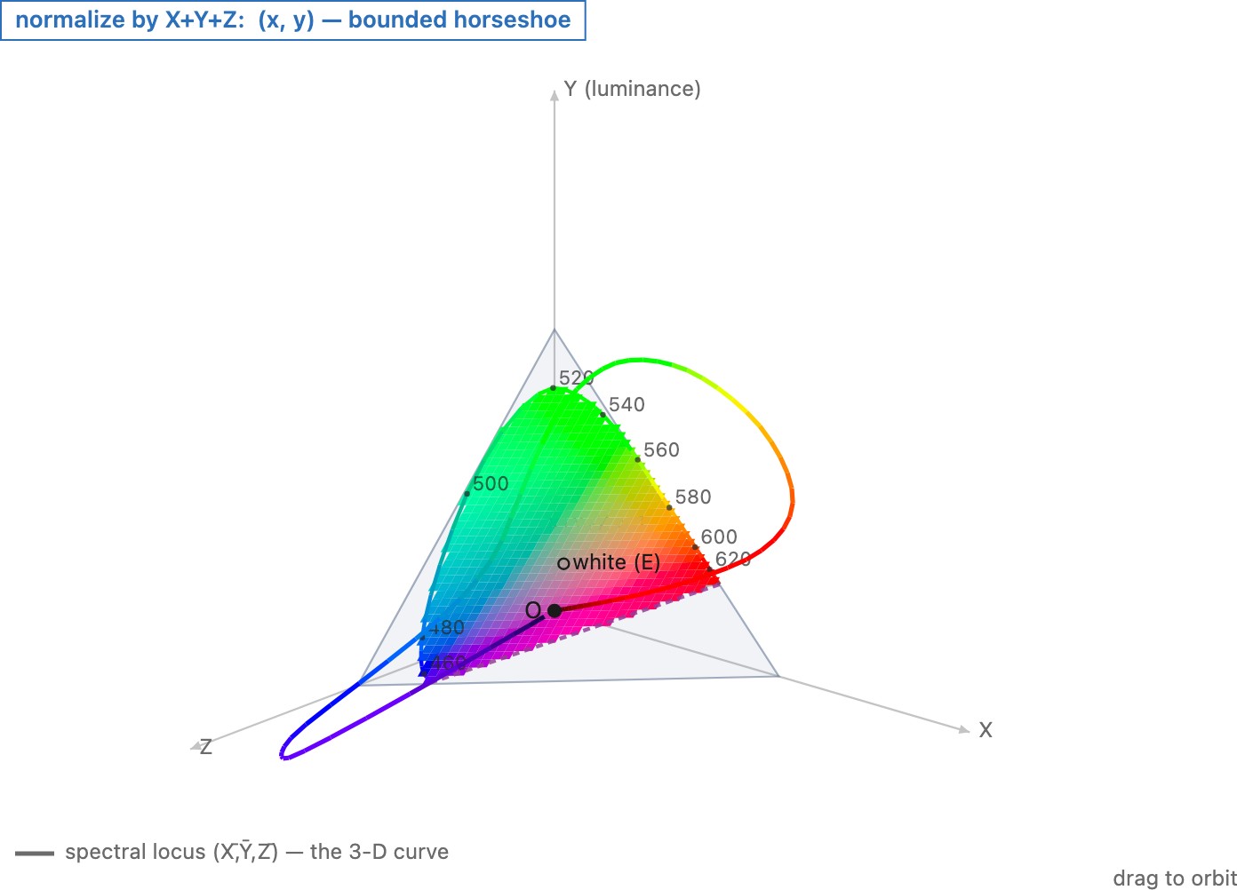
Geometrically, nonnegative spectra project to a cone of realizable tristimulus values Koenderink, Color for the Sciences. Normalizing by $X+Y+Z$ intersects each nonzero ray with a plane. Normalizing by another linear quantity gives a different cross-section. Although the underlying three-dimensional coordinates are related linearly, the normalized two-dimensional coordinates are related projectively.
MacLeod–Boynton chromaticity MacLeod & Boynton, cone-excitation chromaticity diagram (1979) uses cone fundamentals scaled so their L and M components sum to the luminance function. It plots $l=L/(L+M)$ and $s=S/(L+M)$. To interpret a horizontal displacement as an L–M trade at fixed luminance, hold the omitted scale $L+M$ fixed. The coordinates themselves do not force all plotted stimuli to have equal luminance, just as $xy$ does not.
A positive XYZ or LMS triple need not be physically realizable: positivity of three projections is weaker than existence of a nonnegative spectrum producing them. Reflectance introduces further constraints, since it must lie between zero and one under a specified illuminant. Do not confuse this surface-color problem with unconstrained emission.
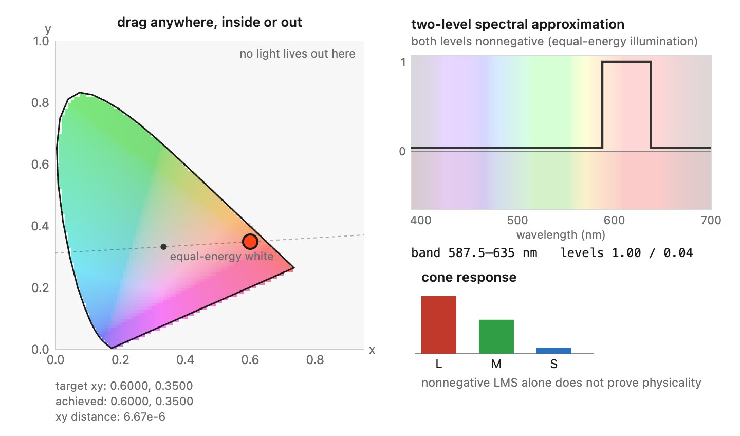
Why divide by the sum rather than by luminance alone? Dividing by $Y$ is an appealing choice when the goal is to separate luminance from color, but coordinates such as $X/Y$ can become very large when $Y$ is small compared with another component. By dividing nonnegative XYZ coordinates by their sum, we instead put each normalized component between zero and one and make the three sum to one. The resulting diagram is bounded. This is a practical benefit of the chosen normalization, not a statement that its distances are perceptually uniform. Figure 4.1.8 makes the choice visible as a change of slicing plane.
The curved locus also has a physical origin. Sweep a monochromatic test through wavelength. At each setting its position comes from the three matching-function values at that wavelength, normalized by their sum. Those values vary together along the sensitivity curves, so the plotted point follows a curve rather than the sides of a triangle. Mixtures fill the convex region determined by that locus. The diagram's outline reflects the observer's spectral sensitivities; it is not an arbitrary shape chosen for a plotting convention.
Keeping track of what the numbers mean⧉
An array needs more than a label saying “RGB.” Record its primaries, transfer function, white reference, numeric range, and whether it represents scene light or a rendered image. Relative XYZ also needs its normalization. A camera-native RGB array needs a camera characterization.
Before a transform, check these assumptions against its input. A matrix defined for linear RGB cannot consume sRGB-encoded samples directly. Assigning a profile declares how existing numbers should be interpreted; converting to another profile changes the numbers to preserve the intended color. White adaptation changes a reference condition and must not be applied twice.
I find this bookkeeping more troublesome than most of the individual equations. Several independent choices travel under one name such as “sRGB,” and applications often hide which choices they made. Explicit metadata and a few labeled intermediate arrays are more useful than guessing from whether the picture looks plausible.
Treat a color transform like a units check. A matrix labeled as taking linear Rec. 709 RGB to XYZ cannot be fed the encoded samples read from an sRGB image. A value labeled Y′ is luma, so substituting it for linear luminance in a physical-light calculation changes the problem. A transform expecting a D65 reference cannot silently be given D50-relative coordinates. Writing the encoding and white reference next to an intermediate array makes these errors visible before the picture is displayed.
There are two kinds of difficulty here. Some come from the measurement: three responses do not determine a spectrum, and the same surface sends different light under different illumination. Others come from conventions maintained across decades, such as print workflows using D50, common display spaces using D65, and the name sRGB covering both primaries and a transfer function. Separating the physical ambiguity from the bookkeeping helps identify what a better calibration can solve and what merely needs an explicit conversion.
A cleaner interface would separate the measurement of the incoming light from the choice of how a particular device should reproduce it. The measurement would identify its observer and normalization; the rendering would specify the viewing conditions, output device, and intended appearance. Color management tries to provide this separation through documented profiles and a common connection space (Chapter 4.8, Recap: the full color pipeline, color management and ICC). It has to work with existing representations, though. A name such as sRGB specifies primaries, a white reference, and an encoding together. Separating those choices remains work for the programmer. The type annotations make that separation explicit on the page.
Linear RGB⧉
LMS and XYZ are analysis spectra, built to measure color. To store and reproduce it we use the RGB family, and the standard member is sRGB (Stokes et al. 1996 (sRGB)), whose primaries are the Rec. 709 primaries under the D65 white point. In linear light, sRGB and XYZ are one $3\times3$ apart. The forward matrix takes a measured color into linear sRGB,
and its inverse recovers XYZ,
The coefficients shown are rounded. Apply them to linear values; a typical sRGB file must first be decoded. The middle row of the RGB-to-XYZ matrix gives relative luminance. Applying those weights to encoded components gives luma, which is neither luminance nor generally the encoding of luminance.
Negative RGB components indicate a target outside the positive cone spanned by these primaries. Components above one exceed the chosen reference range; they can represent greater intensity at an otherwise reproducible chromaticity. Floating-point scene-linear images often retain such values. Clipping to $[0,1]$ is an output decision that can change hue and discard highlight information.
RGB color spaces⧉
An RGB space chooses primary chromaticities and a reference white; its stored representation also specifies a transfer function. Different choices serve different devices and workflows. sRGB is a common SDR delivery space. Display P3 extends its red and green coverage. Adobe RGB extends especially into greens and cyans useful in some print workflows. Rec. 2020 has still wider primary chromaticities. ProPhoto is a large working space with imaginary primaries.
With fixed integer precision, a larger gamut generally spreads codes more widely in color. The effect varies across the gamut and depends on the transfer function. Use sufficient precision for editing, then choose the delivery space from the output requirements. A screen cannot display every working-space value merely because software can store it.
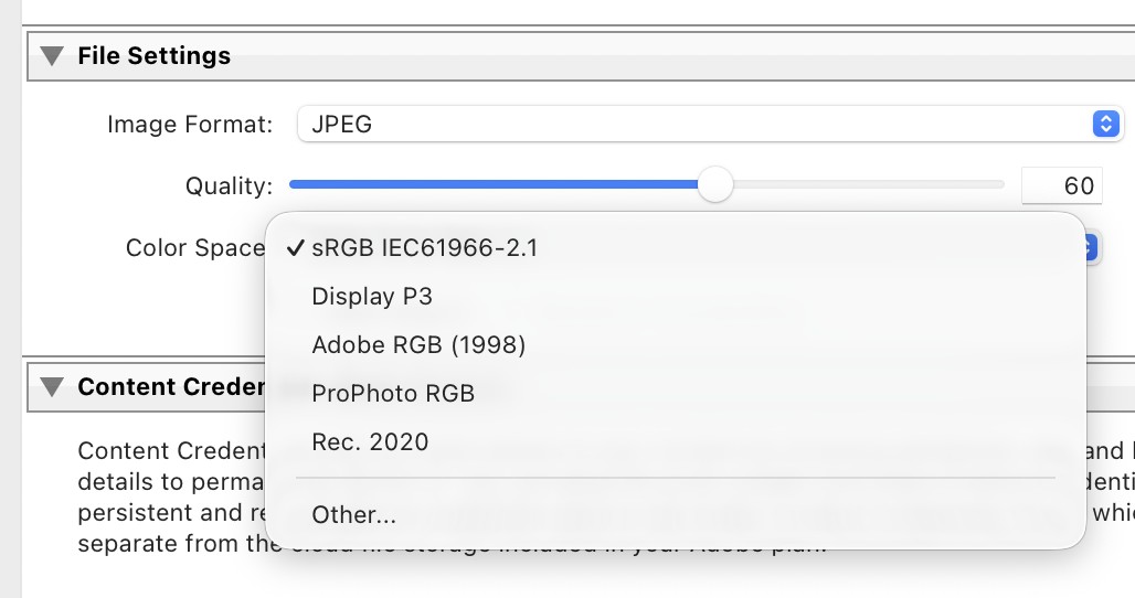
Choose a working gamut large enough for the content and operations, with sufficient numeric precision. Choose a delivery space the receiving system can interpret. Wider primaries alone do not improve an image, and converting an sRGB image to a wider space does not recover colors previously clipped.
Display-oriented spaces describe a reference set of primaries. Working spaces can instead choose imaginary primaries to enclose more physical colors. ProPhoto’s green and blue are outside the spectral locus; its red is not the imaginary pair’s other member. Such coordinates are useful for calculation, but their nonnegative cube contains values no physical light can produce.
Camera raw is different. Its channels are spectral measurements, often one color sample per photosite in a mosaic, not weights of three emission primaries. A camera would admit an exact universal XYZ matrix if its sensitivities spanned the standard observer’s matching functions. Real cameras generally only approximate this condition, so color correction is fitted and depends on spectra and illumination. It is not meaningful to invert an arbitrary three-by-many sensitivity matrix and call the result three physical display primaries.
Camera profiles can provide multiple illuminant calibrations. Do not assume every DNG contains exactly two matrices at fixed temperatures; use the tags and conventions of the actual profile. Camera color-space menu settings usually govern rendered output and previews, while raw channel interpretation remains camera-specific.
The correction matrix also propagates noise. With equal independent input variances $\sigma^2$, output channel $i$ has variance $\sigma^2\sum_j M_{ij}^2$. More generally use $M\Sigma M^T$. Negative coefficients do not alone prove amplification; their magnitudes and the input covariance matter. The filter design and color fit balance sensitivity, color accuracy, and noise, as developed in Chapter 4.6, Sensing color: multiplexing strategies.
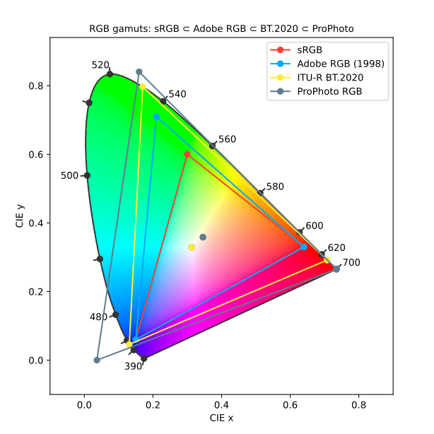
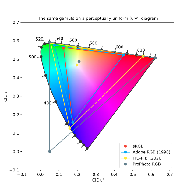
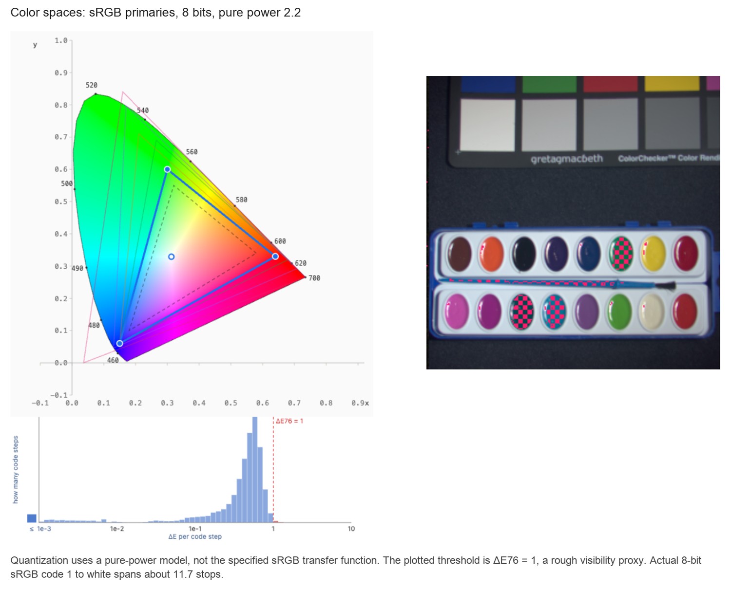
This distinction explains two different kinds of color-conversion experiment. Between linear RGB working spaces built from the same standard observer, convert a color to XYZ and then to the destination coordinates; the two matrices compose into one exact coordinate transform. For a camera, photograph a set of known reflectances under a specified light and fit a matrix from the measured camera responses to their target XYZ values. It can fit those samples well and still make errors on other spectra. Two spectra that the camera records identically cannot be separated by any later matrix, even if the standard observer distinguishes them. More training patches improve the fit over a chosen population; they do not restore spectral information absent from the three measurements.
The choice of a working gamut also affects quantization. With a fixed integer bit depth, a wider set of primaries spreads the available code combinations over a larger range of colors. It can retain a saturated color that a smaller space clips, yet give coarser steps in a region shared by both spaces. Increasing bit depth or using floating point reduces that pressure. This is why a space suited to intermediate editing need not be the best choice for compact delivery. The working space must retain the colors the pipeline needs; the output space must match the interpretation supported by the destination.
A caution about that diagram before we read too much into the triangle sizes: the $xy$ chromaticity plane is a space for measuring color, not for judging how different two colors look. It stretches the greens enormously and cramps the blues and purples, so neither the relative areas of these gamuts nor the distances between their primaries track perceived difference. Re-plot the identical primaries on a perceptually more uniform diagram, the CIE 1976 UCS ($u'v'$) space, and every triangle changes shape (Figure 4.4.3): the relative areas and distances change. The newer diagram is more uniform, but it is still not a universal perceptual ruler. That $XYZ$ (and its $xy$ projection) is not perceptually uniform is precisely what will force the deliberately non-linear spaces of Chapter 4.5, Advanced color: opponents, perceptually-uniform, and preferred.
Two design processes can lead to an RGB space. In a display-oriented design, begin with the primaries a reference display can emit, then describe colors as amounts of those lights. In a working-space design, begin with the colors that editing should retain, then choose a coordinate system that encloses them. The latter need not correspond to a manufacturable display. An imaginary primary is acceptable as a coordinate axis because no lamp is being asked to emit it while the image is stored or edited. Physical realizability becomes an output constraint when those values are converted for a screen or printer.
This distinction explains why choosing a larger working space does not upgrade the monitor. It changes which intermediate colors can be represented without clipping to the working cube. Displaying them still requires conversion and, where needed, gamut mapping. Conversely, a delivery space can be chosen for compatibility with the intended viewing path even when a larger space was useful during editing. The export dialog asks for an engineering choice about that destination, not a ranking in which the largest triangle is always best.
The noise formula can be read numerically. A correction row with coefficients 1.8, -0.9, and 0.1 has squared length 4.06. With equal independent input noise, its output standard deviation is therefore about 2.01 times the standard deviation of one input channel. The row may improve the color fit while increasing that channel's noise. This is why a camera characterization should be evaluated for both reconstruction error and noise propagation, using the actual covariance rather than assuming that every color matrix has the same cost.
Two different words for impossible⧉
optionalA chromaticity can be physically realizable yet outside a display’s primary triangle. Conversely, an RGB space with imaginary primaries can encode chromaticities no nonnegative spectrum produces. These are different limitations. Signed floating-point RGB can also represent colors outside its positive-primary triangle, provided subsequent operations preserve the signed values.
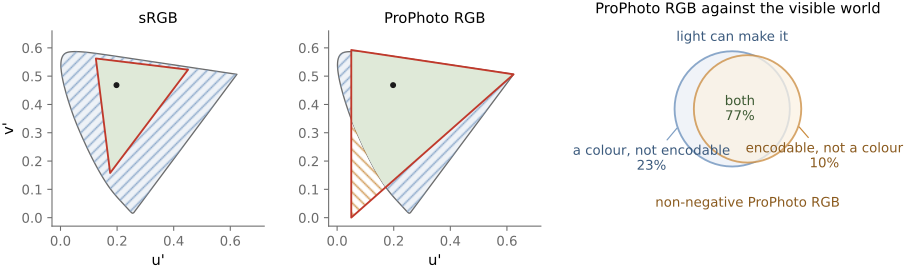
A chromaticity triangle omits luminance. Even a chromaticity inside the triangle may require more light than a display can emit at the requested luminance. Similarly, reflectance is bounded by one: under fixed broadband illumination, pushing a surface color toward a spectral endpoint usually restricts the wavelengths it reflects and reduces its possible luminance. This helps explain the shape of the object-color solid, but does not imply that ordinary pigments always fit sRGB. Saturated flowers, paints, fabrics, structural colors, and colored lights can require gamut mapping.
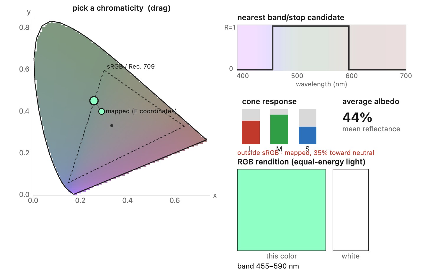
The RGB cube shows the bounded encoding in three dimensions. Its geometry depends on whether its coordinates are linear or nonlinear; its Euclidean distances are not perceptual color differences.
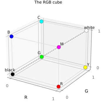
The optimal-reflectance experiment makes the brightness constraint concrete. Under a fixed broadband light, an ideal white reflector returns light across the whole spectrum. Restricting reflection to a narrow wavelength interval rejects the power outside that interval. The resulting chromaticity can be very saturated while the available reflected luminance becomes small. An emitter need not pay this same price: it can put substantial power directly into a narrow band. This is a reason to distinguish surface-color limits from the gamut of colored lights. It does not imply that all colors outside sRGB are nearly monochromatic or that saturated ordinary materials can be ignored.
Reference: primaries, matrices, and transfer functions⧉
optionalEach space named above is fixed by two things: its primaries and white point, which set the linear RGB-to-XYZ matrix, and its transfer function, the gamma curve that encodes the linear values for storage. The matrices below carry linear light, no diacritic, into $\mathrm{XYZ}$; the transfer is applied afterward to get the stored $R'G'B'$ (the primes of Chapter 4.3, Encoding: linear, gamma or log). The middle row of each matrix is that space's luminance $Y$ weighting, the coefficients also used, with the specified nonlinear encoding, to define a corresponding luma (L4.5).
sRGB and Rec. 709 primaries (D65) share this linear matrix, though their transfer conventions differ:
sRGB transfer: piecewise, a linear segment $R' = 12.92\,R$ for $R \le 0.0031308$ splicing into $R' = 1.055\,R^{1/2.4} - 0.055$, overall close to $\gamma = 2.2$.
Adobe RGB (1998) (D65), wider greens for print work:
Transfer: a pure power law, $\gamma = 2.19921875$ (that is $563/256$).
Display P3 (D65), the DCI-P3 primaries on the sRGB white:
Transfer: the sRGB piecewise curve.
ITU-R BT.2020 / Rec. 2020 (D65), ultra-high-definition with very wide primaries (its red is a near-monochromatic 630 nm):
Transfer: BT.2020 specifies a camera-side piecewise encoding with a 0.45-power segment and linear toe. Specify the display response separately. Rec. 2100 uses the same primary chromaticities with PQ or HLG HDR systems (Chapter 4.3, Encoding: linear, gamma or log).
ProPhoto RGB (ROMM) (white point D50), a large editing space with imaginary green and blue primaries:
Transfer: $\gamma = 1.8$, with a short linear segment (slope $16$) below $R = 1/512$.
Two reminders the type system enforces. The matrices are all defined on linear light, so a conversion between two of these spaces is $M_2^{-1} M_1$ applied to linear RGB, never to the stored $R'G'B'$: decode first. And the white points are not all the same (ProPhoto is D50, the rest D65), so a white-relative ProPhoto-to-sRGB conversion includes chromatic adaptation (often Bradford, Chapter 4.2, White balance and white point) between the XYZ stages. A stimulus-preserving conversion has a different objective and does not silently adapt the white.
For a white-relative conversion, the full order is
linear_source = decode_source(encoded_source)
XYZ_source = M_source @ linear_source
XYZ_target = adapt_white(XYZ_source, source_white, target_white)
linear_target = solve(M_target, XYZ_target)
# Retain extended range while working; map gamut for the chosen output.
encoded_target = encode_target(mapped_linear_target)
The printed matrices are rounded reference values. Use a consistent precision and white normalization in code. Verify that RGB white maps to the stated XYZ white and that an unmodified in-gamut round trip returns its input.
Sensing color: multiplexing strategies⧉
Spectral sensitivity: matching the eye, catching photons, and white balance⧉
optionalWith photon spectral exposure $q(\lambda)$ and effective channel detection probability $\eta_i(\lambda)$, the expected signal electrons are
The response includes filters, optics, and quantum efficiency under the stated convention. Sampled implementation needs wavelength-bin weights. Shot noise is determined by detected electrons, while read noise is added by the readout; the full model is in Chapter 2.8, Noise, signal-to-noise ratio and dynamic range. A broad response alone is not a color measurement: distinct response shapes supply the information that separates spectra.
The exact shape of a color sensor's three spectral-sensitivity curves (the $r(\lambda)$ of the red, green, and blue channels, built earlier by the color-filter array on the photosites of Chapter 2.7, Sensors: photosites, CCD vs CMOS) is one of the camera's most constrained choices, because it is pulled in three directions at once that cannot all be satisfied.
- Fidelity to human vision. For a camera to record the color a human would see, its three curves should be a fixed linear combination of the eye's cone fundamentals (equivalently, of the CIE color-matching functions), the Luther–Ives condition. A sensor that met it could be mapped to human color by a single $3\times3$ matrix with no error. Practical camera sensitivities generally only approximate it, because silicon-plus-dye curves are simply the wrong shape, and the penalty is a metameric error no color matrix can remove: two spectra that look identical to the eye read as different RGB, and two that look different can read the same. The color-correction matrix in Chapter 8.10, Auto-exposure and auto white balance is a least-squares compromise: right on average, wrong on the hard cases (saturated reds, narrow-band LEDs, foliage).
- Quantum efficiency and noise. Broad transmission bands can increase total photon collection; this is distinct from quantum efficiency at a specified wavelength: the wider each filter, the more photons reach the well and the higher the SNR. Strong overlap can make color separation poorly conditioned, because separating similar channel responses can require large signed coefficients that amplify measurement noise (compare the distinct physiological opponent processing in Chapter 3.2, Perceptual color and trichromatic vision). Narrow, well-separated filters give clean color but throw photons away and read noisier. The green-doubled Bayer is one point on this curve: spend photons and resolution where the eye cares most (luminance), economize on chroma.
- White balance across illuminants. Because each channel integrates illuminant × reflectance × sensitivity, changing the light changes the raw RGB of a fixed object. Undoing that, white balance often approximates the change with per-channel gains. Matching cone sensitivities does not make this diagonal relighting model exact; a response set that matches human colorimetry well need not be the best basis for diagonal adaptation. Good spectral design makes white balance more reliable across illuminants (→ Chapter 8.10, Auto-exposure and auto white balance).
These three pull against each other: the curves that best match the eye are broad and overlapping (bad for separation), the curves that separate color cleanly are narrow (bad for QE and for matching the eye), and keeping white balance stable across odd illuminants wants yet another shape. Every color sensor is a negotiated settlement among them (Figure 4.6.24).
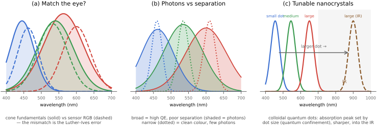
Synthesizing color⧉
optionalSensing a color projects a spectrum onto three numbers; synthesizing one runs that backward, building light from a few primaries so that a human sees the intended color. The projection threw information away and cannot be undone, so synthesis does not rebuild the original spectrum, only a metamer of it, and it must do so with real lights or real inks, which can only add or absorb, never contribute a negative amount. That single constraint, non-negativity, shapes everything in this chapter: which colors a device can reach (its gamut), what has to happen to the ones it cannot (gamut mapping), and how displays, printers, and film each make their compromise with it.
Additive vs subtractive⧉
optionalSynthesis, building a color from primaries, is where the constraints of non-orthogonality and non-negativity become concrete. Suppose we want to reproduce a single monochromatic test color, a pure wavelength, using three fixed primaries (Figure 4.7.1). In the linear-algebra picture this is asking for weights $w_i$ such that $\sum_i w_i \mathbf{P}_i$ matches the target. The 2-D analogy makes the trouble plain: with two non-perpendicular basis vectors you can reach any point in the plane if you are allowed negative coefficients, but a primary is a light, and you cannot emit a negative amount of it. So the reachable colors are not the whole plane but only the convex cone of non-negative combinations. Non-orthogonality plus non-negativity turns some perfectly real colors into impossible reproductions: the saturated cyans that needed negative matches in the color-matching experiment simply cannot be made by adding three real primaries.
Concretely, stack the three primaries as the columns of a matrix $P$, each column a primary's tristimulus, so $P$ has the signature $P : \mathbf{w} \to \mathrm{XYZ}$ (weights in, a color out). An additive mixture is a non-negative weighted sum, and reproducing a target $\mathbf{c}$ is one solve:
For ideal independent primaries with maximum drives normalized to one and zero black offset, the target is reachable when $0\le w_i\le1$ for every channel. Nonnegativity alone describes an unbounded intensity cone. The gamut is that constraint drawn out: the convex cone $\{P\mathbf{w} : \mathbf{w} \ge 0\}$, which on the chromaticity diagram (tristimulus-normalized) is the triangle of the primaries. A weight forced negative is the non-negativity wall, a real color the device cannot make. These weights specify linear primary intensities. Converting them to hardware codes requires the calibrated inverse of the device’s code-to-light response.
Nonnegative mixtures of fixed additive primaries lie within their chromaticity hull. Three primaries give a triangle. Maximum drive and black level also constrain the full three-dimensional gamut. Subtractive printing is not described by the same triangle rule: ink interactions and the paper must be characterized.
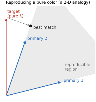
There are two physically distinct ways to mix color, and the distinction is more subtle than the names suggest. Split the spectrum into three coarse bands and pretend they are pure B, G, R (Figure 4.7.2). Additive mixing (lights) starts from black and adds bands: $R + G + B$ gives white, and the pairs give yellow, cyan, magenta. Subtractive mixing (filters and inks) starts from white and each layer removes a band, with cyan, magenta, yellow stacking toward black. But "subtractive" is a misleading name: stacking filters is really a wavelength-by-wavelength multiplication of the spectrum.
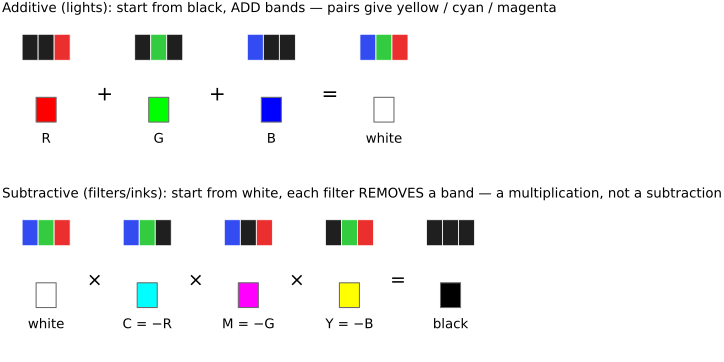
This is easy to see with filter transmittances. A yellow filter blocks blue; a cyan filter blocks red. Stack them and the only band that survives is the overlapping green, so yellow $\times$ cyan = green, which is a product of the two transmittance spectra $T_Y(\lambda)\cdot T_C(\lambda)$, not any kind of sum (Figure 4.7.3). In general a stack of dyes multiplies transmittances wavelength by wavelength,
a product that in log transmittance (optical density) becomes a sum, which makes density useful for ideal dye-layer calculations and why "subtractive" is a misnomer for a multiplication. The overlapping-disks picture captures both regimes at a glance: RGB lights overlapping toward white versus cyan-magenta-yellow (CMY) inks overlapping toward black (Figure 4.7.4). And real systems are often hybrid: an LCD projector, for instance, uses a white lamp, panels that subtract (modulate) each channel, and then adds the three channels on the screen.
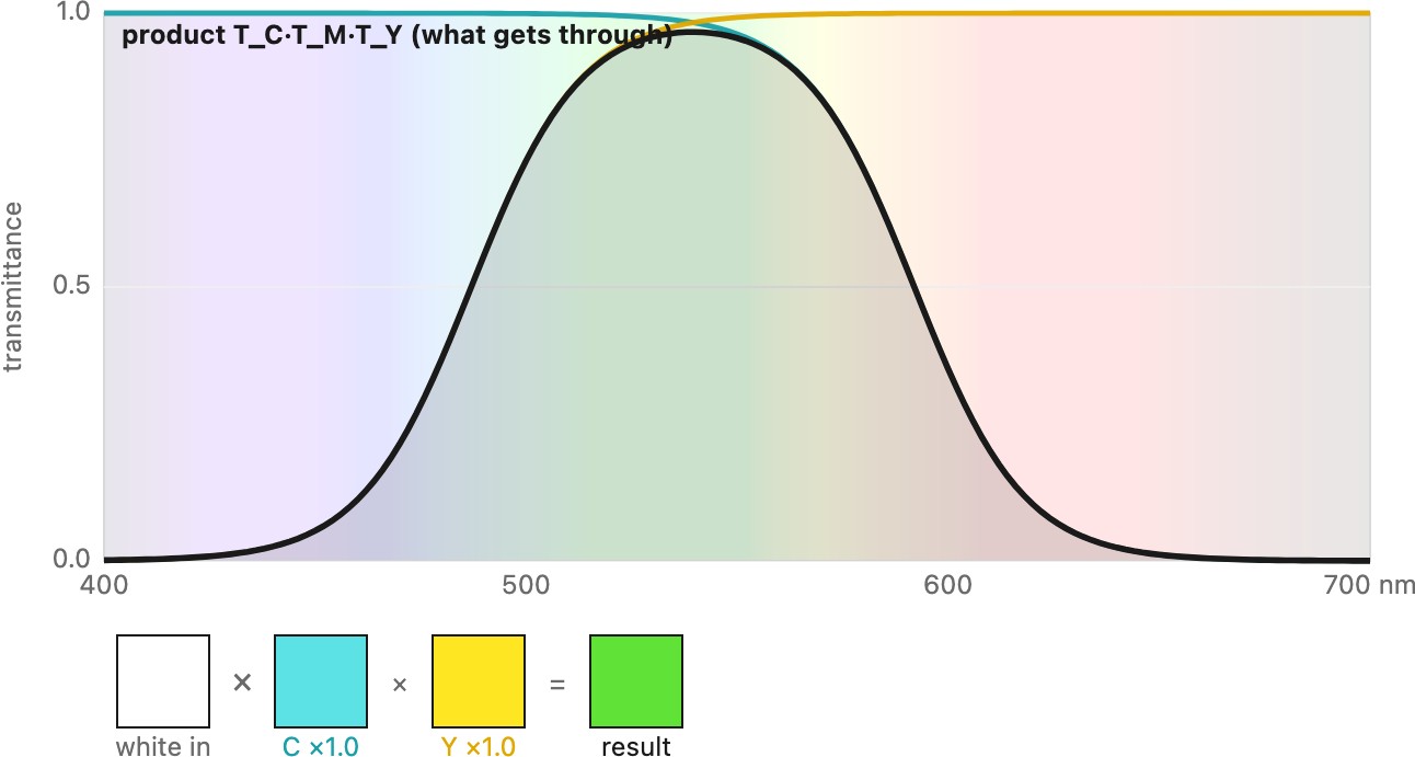
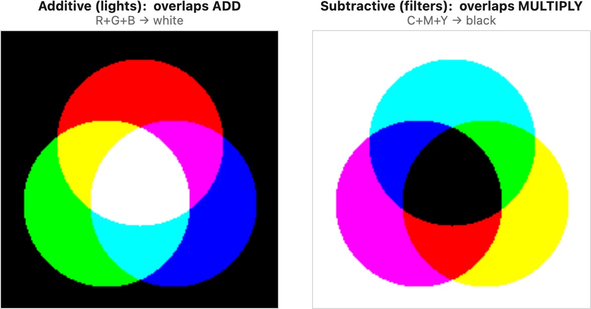
CRTs and OLEDs emit light; LCDs modulate a backlight through filters. Their subpixel outputs mix additively at viewing distance. Printed layers absorb and scatter light, while halftone areas also mix spatially. The ideal transmittance product assumes independent non-scattering layers and neglects interface reflections; a print needs a more complete model or measured profile.
Gamut and gamut mapping⧉
optionalThe destination has a bounded set of reproducible tristimulus values. A chromaticity diagram shows part of that limit, but a target can lie inside the primary triangle and still demand excessive luminance. Use the full gamut for output decisions.
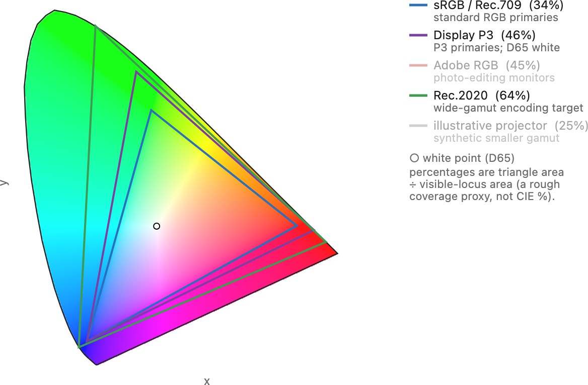
Gamut mapping changes colors the destination cannot reproduce, and may also change nearby in-gamut colors to preserve smooth variation. Channel clipping is cheap but can change hue and collapse distinct colors. Nearest-boundary mapping depends on the distance metric. A line toward white in xy does not generally preserve perceptual hue or lightness.
One simple perceptual-coordinate construction holds Lab lightness and hue fixed and reduces chroma:
This assumes the destination has a feasible neutral and chroma interval at that lightness. If it does not, lightness must change too. A soft compression replaces this hard limit with a continuous function that also moves some in-gamut values. No mapping preserves every original difference when the output gamut is smaller.
A nearest-color formulation is
with destination gamut $\mathcal G$ and a stated color-difference measure $d$. This need not agree with channel clipping or constant-hue chroma reduction. Choose by the image and output objective, then inspect saturated texture, gradients, and important colors. A brand color outside the output gamut cannot be made exact by selecting a different clipping rule.
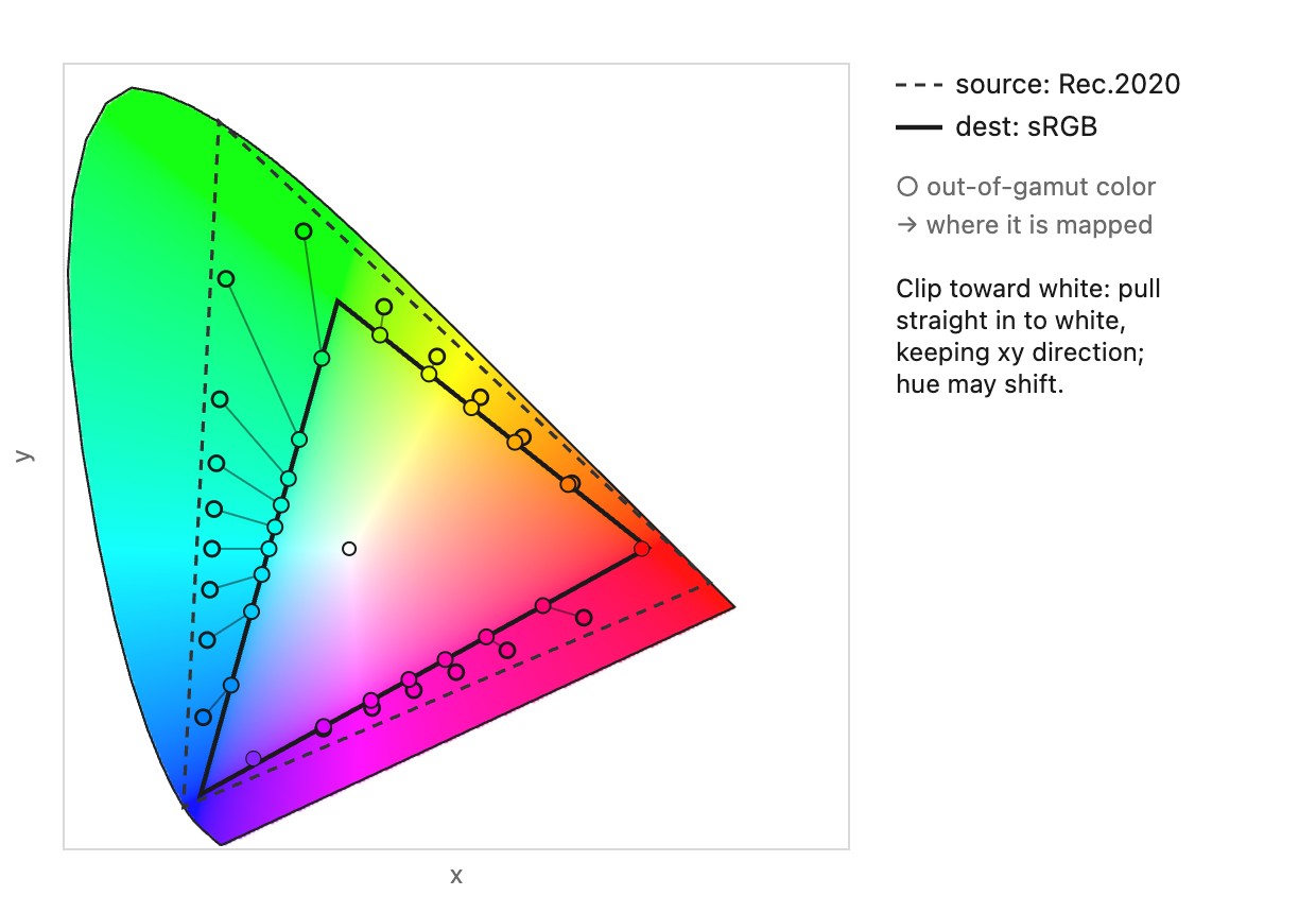
ICC rendering intents describe conversion objectives rather than one universal clipping or compression algorithm. Their results depend on profiles and the color-management module; see Chapter 4.8, Recap: the full color pipeline, color management and ICC.
Imagine a red channel that rises smoothly from 0.9 through 1.1 to 1.3 while the other channels remain fixed. Clipping that channel at 1 preserves the first part of the ramp but makes all its higher values identical. Any texture encoded only by those differences disappears. A compression that begins before the boundary can retain distinctions among the higher values, at the cost of changing some values that were already reproducible. This is the practical choice behind the two families: where to spend the available color differences. The mapping's color space and trajectory also matter, because preserving a straight line in chromaticity coordinates does not guarantee constant perceptual hue.
Color TLDR⧉
Physical color⧉
Before any eye or sensor, color is physical: a light is a spectrum, its power at each wavelength (the spectral power distribution). For a surface, the light that reaches the eye is not the surface's own but the illumination times what the surface reflects, $C(\lambda) = S(\lambda)\,\rho(\lambda)$: the illuminant spectrum $S(\lambda)$ multiplied wavelength by wavelength by the surface reflectance $\rho(\lambda)$. An apple looks red because its reflectance is high in the reds and low elsewhere, but only when there is red light to reflect: under a pure green lamp the same apple is nearly black. Self-luminous things (a screen, a flame, the sky) skip the product and emit their spectrum directly. Everything after this reduces that spectrum to a few numbers. Details: Chapter 4.1, Linear color reproduction and CIE XYZ.
Cones, LMS, and metamerism⧉
The eye has three types of color-sensitive photoreceptors. Given a physical spectrum, their response $L, M, S$ is a projection (dot product) of the light onto three sensitivity curves. That is, it's the integral of the light spectrum times the sensitivity of each cone. Because the sensitivity curves overlap, the three axes, $L, M, S$, are non-orthogonal (there is cross-talk), and because light cannot be negative, not every point is reachable. And because only three numbers survive, many different spectra collapse to the same triple: metamers. That is, metameters are different physical spectra that project on the same $L, M, S$, and are therefore perceived as the same color. This is exactly what lets a three-primary screen reproduce any color. Details: Chapter 4.1, Color space 101.
XYZ⧉
In an ideal world, color science would be built on $L, M, S$, but for historical reasons (it took a while to have technology to measure cone responses), the standard we all build on is CIE XYZ. It is a linear transform of LMS, one $3\times3$ matrix away; its coordinates are semi-arbitrary, with one exception, $Y$ is defined to be luminance. It was originally built through color reproduction experiments rather than by measuring cones, but you do not need that history to use it: treat XYZ as the standard, device-independent coordinate system everyone converts through. Details: Chapter 4.1, Color space 101.
Chromaticity and gamut⧉
For visualization purposes, it is convenient to drop brightness and use a 2-D chromaticity diagram. The standard version starts with XYZ and divided by the sum of the three numbers. Physically realizable colors (spectra with no negative light) occupy a horseshoe shape with monochromatic light at the boundaty. A device's reproducible colors, the mix of its primaries, form a convex region (a triangle for three primaries) inside it: its gamut. Colors outside the triangle cannot be made and must be mapped in, which is called gamut mapping. Details: Chapter 4.1, Color space 101, Chapter 4.7, Synthesizing color.
Linear RGB, and why there are many⧉
There are many named RGBs (sRGB, Adobe RGB, Display P3, Rec.2020, ProPhoto). Getting to one RGB space from XYZ is again a single $3\times3$ matrix.
People define different RGBs for three practical reasons: different display primaries (so different gamuts), and different trade-offs of bit budget and bandwidth (a wider gamut spreads the same bits thinner). Pick by what you need to cover and how many bits you can spend. Details: Chapter 4.4, RGB color spaces.
Color terms⧉
Radiometry: physical light, no observer⧉
Radiometry. The physical measurement of light as electromagnetic power, with no reference to a human observer.
Radiance. Power per unit projected area per unit solid angle, in W·sr⁻¹·m⁻². The fundamental quantity a camera measures, and the one preserved along a ray through empty space; sensor- and observer-independent. Written $L$ (linear).
Irradiance. Power per unit area arriving on a surface, in W·m⁻². What the sensor plane actually receives; it is tied to scene radiance through the lens by the aperture (f-number) and the projection geometry. Written $E$.
Spectral radiance. Radiance per wavelength interval, $L(\lambda)$, with units such as W·sr⁻¹·m⁻²·nm⁻¹. A spectral power distribution (SPD) describes power or another specified radiometric quantity versus wavelength; state which quantity and normalization. A spectrum alone does not specify the spatial, angular, temporal, or polarization distribution of light.
Photometry: physical light weighted by the eye⧉
Photometry. Radiometry weighted by the human luminosity function $V(\lambda)$, the daytime spectral sensitivity of vision. It defines standard observer-weighted physical quantities, not a complete prediction of perceived brightness. Other photometric regimes use other specified weightings.
Luminous flux. Total light power weighted by $V(\lambda)$, in lumens.
Luminance. The photometric counterpart of radiance: radiance weighted by $V(\lambda)$, in cd·m⁻². A linear weighted integral of spectral radiance; it is not proportional to total photon count independently of spectrum. It correlates with brightness but is not itself a percept. Written $Y$ in XYZ (or $L$ where context is clear). Physical color mixing can operate on full linear RGB or spectra; luminance alone discards chromatic information.
Illuminance. The photometric counterpart of irradiance, the luminous flux arriving per unit area, in lux.
The chronic confusion, luminance $Y$ vs luma $Y'$: $Y$ is linear, photometric and device-independent; $Y'$ is computed from specified nonlinear $R'G'B'$ and depends on the encoding and coefficients; it is generally not the encoding of $Y$. Same letter, different domain, different meaning (L4.5).
Colorimetry: color via the standard observer⧉
Colorimetry. The measurement of color, made repeatable by fixing a standard observer whose sensitivities stand in for a human's.
Color-matching functions (CMFs). $\bar x(\lambda),\ \bar y(\lambda),\ \bar z(\lambda)$: the CIE 1931 standard observer's three sensitivity curves, measured empirically from color-matching experiments. They are the mechanism by which a spectrum is projected onto three numbers.
Tristimulus values. $X, Y, Z$: the three numbers from integrating the SPD against the CMFs over wavelength with a specified normalization. They are linear in the stimulus; $Y$ is relative luminance or absolute luminance according to the scale.
Metamerism. Two different spectra that integrate to the same XYZ for a given observer, and match under the specified viewing conditions. Camera metamerism can differ from standard-observer metamerism. Surface matches can change with illumination, whether or not the illuminant is spiky.
Chromaticity. Tristimulus coordinates with overall scale removed: $x = X/(X{+}Y{+}Z)$, $y = Y/(X{+}Y{+}Z)$. A projective quantity, reduced from three dimensions to two, so it names a color's direction but not its amount and cannot be turned back into XYZ without $Y$ supplied separately.
Chromaticity diagram. The 2-D plot of $x,y$ (or the more uniform $u',v'$) chromaticities, the horseshoe. Three-primary additive gamuts project to triangles and the blackbody illuminants as the Planckian locus.
Spectral locus. The curved boundary of the horseshoe, the chromaticities of monochromatic (single-wavelength) lights. For ordinary broadband illumination, a bounded surface reflectance approaching a spectral endpoint generally has a low maximum luminance.
Line of purples. The straight edge closing the horseshoe between the red and violet ends of the spectral locus. Its colors are real but have no single-wavelength equivalent; they are mixtures of the two spectral extremes.
Chronic confusions, named⧉
Nine pairs this part keeps apart, and the distinction in each:
| term | vs | the distinction |
|---|---|---|
| luminance $Y$ | luma $Y'$ | linear photometric quantity vs weighted nonlinear components |
| lightness $L^*$ | luminance $Y$ | perceptual correlate vs linear photometric quantity with a stated scale |
| chroma $C^*$ | $C_b,C_r$ | perceptual magnitude in CIELAB vs encoding difference signals |
| saturation | chroma $C^*$ | relative to the object's brightness vs relative to white |
| chromaticity $x,y$ | color $XYZ$ | projective 2-D (luminance discarded) vs full 3-D |
| white point (space) | white balance (camera) | a mathematical normalization vs illuminant compensation |
| OETF | EOTF | camera encoding vs display decoding |
| colorfulness | chroma $C^*$ | absolute percept vs white-relative percept |
| primaries | phosphors / LEDs | abstract basis vectors vs physical emitters |
One word, several meanings⧉
A few terms carry different meanings in different chapters and are worth disambiguating on sight:
White point has four senses: a color-space normalization parameter, a display's calibration target, a viewer's adaptation state, and a camera's auto-white-balance target. They are designed to agree in a calibrated pipeline but are conceptually independent.
Color temperature is the temperature (in kelvin) of the blackbody whose glow matches a light's color, so it is only exactly meaningful on the Planckian locus; it is used loosely for any illuminant's chromaticity, and as a camera white-balance control even for non-blackbody sources. Correlated color temperature specifies a nearby Planckian-locus temperature; it does not specify the source spectrum or its off-locus distance.
Neutral means achromatic under specified conditions. Equal RGB components represent the defined RGB white chromaticity; equal XYZ represents equal-energy white, not every neutral. Equal LMS is a normalization-dependent convention, not a general test of neutrality.
Linear can mean proportional to physical light (radiometrically linear), a linear-algebra operation (a matrix, no nonlinearity), or a 1-D sensor layout (a linear array). It always needs its context.
Recap: big lessons in this lecture
Light, and the physical color it carries, is described by a spectral distribution: the power it carries at each wavelength, a function $S(\lambda)$. One wavelength is a single pure color; real light is a weighted mix of all of them. Everything downstream (how a prism fans light out, how a surface reflects it, how a sensor or an eye turns it into a perceived color) starts from this per-wavelength power.
The refractive index is not a constant: $n(\lambda)$ depends on wavelength: in ordinary glass it rises toward the blue, so blue bends more than red. Because of this you cannot route every wavelength the same way with a single refraction: a prism fans white light into a spectrum, a raindrop makes a rainbow, and a simple lens focuses blue and red at slightly different distances: chromatic aberration. Much of the craft of lens design (combining crown and flint glass into achromatic and apochromatic groups) exists to fight this one fact. Dispersion is not a defect of cheap glass; it is built into how matter and light interact.
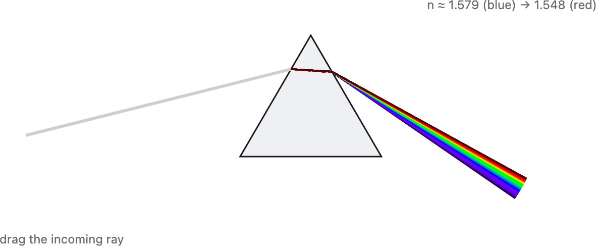
Much of imaging is multiplicative, not additive. The light reaching the eye is illumination times reflectance; contrast is a ratio of intensities; a shadow darkens a region by a factor, not by subtracting a constant. Because the structure is multiplicative, the natural tools are multiply, divide, and log, not just add. This is why, again and again, we will work with ratios and with logarithmic encodings rather than raw linear values. It is also why white balance is hard: to recover an object's true color we must divide out the unknown illuminant $S(\lambda)$ from the product $C(\lambda)$, undoing a multiplication we never observed directly. (The additive counterpoint, light from different sources adding, and what it means for choosing an encoding, comes in Color technology.)
Each cone excitation is an integral of spectral density times the appropriate sensitivity. A sampled implementation must include wavelength-bin widths (or absorb them into the matrix). Three excitations summarize photopic color matching for a fixed observer and viewing condition; they do not recover the spectrum.
Different spectra can yield the same cone excitations for a specified observer. This enables color reproduction without reproducing the spectrum, but a fixed display can match only colors within its gamut. Matches between reflecting materials can fail when the illuminant changes.
A metameric match is a match between two products of reflectance and illuminant (L2.6). Swap the illuminant and you multiply by a different spectral shape, so two surfaces that looked identical under one light can diverge under another: illuminant metamerism. It is the headache behind prints that shift between the proofing booth and the living room, and fabrics that match in the shop but clash in daylight; color-critical work must always name the light a match is judged under.
Cone excitations are followed by neural comparisons and adaptation. Sum-and-difference models illustrate this processing, but their axes are not exact perceptual hue axes. Engineering luma/chroma transforms exploit related sensitivity differences without reproducing the neural pathway.
Specify the purpose when naming primaries: sources whose light is added, inks or filters that absorb light, or perceptual hue judgments. RGB and CMY describe common engineering choices, not unique sets required by nature. The chosen spectra and mixing process determine what can be reproduced.
Cone sensitivity curves overlap, and physical spectra and emitted primary powers are nonnegative. Cone responses are measurements, not spectrum coefficients. Matching a response triple with three primary lights requires solving for their powers; a negative solution identifies a color outside those primaries' additive gamut.
Sensitivity curves measure a spectrum; emission primaries construct one. Reusing the sensitivity curves as primaries and the measured responses as weights generally gives the wrong color. Calibrate how each primary stimulates the observer, then solve for its weight.
XYZ, a compatible LMS system, and linear RGB are different coordinates for a fixed observer’s three-dimensional color matches. Nonlinear RGB encodings and perceptual spaces add specified nonlinear transforms. A real camera’s raw measurements usually require an approximate color correction; an appearance model also needs viewing conditions.
Choose a working gamut large enough for the content and operations, with sufficient numeric precision. Choose a delivery space the receiving system can interpret. Wider primaries alone do not improve an image, and converting an sRGB image to a wider space does not recover colors previously clipped.
Nonnegative mixtures of fixed additive primaries lie within their chromaticity hull. Three primaries give a triangle. Maximum drive and black level also constrain the full three-dimensional gamut. Subtractive printing is not described by the same triangle rule: ink interactions and the paper must be characterized.