Lecture Notes 2 — Convolution⧉
Course notes cut from Computational Photography, an AI-powered Slopendium for this lecture. Each section links back to its home in the book; sections marked optional go beyond what the lecture needs.
Contents · 34 sections on this page, from 12 chapters of the book
Titles jump to the section below; ↗ opens it in the book.
Light and optics⧉
Wave effects, diffraction, and the diffraction limit⧉
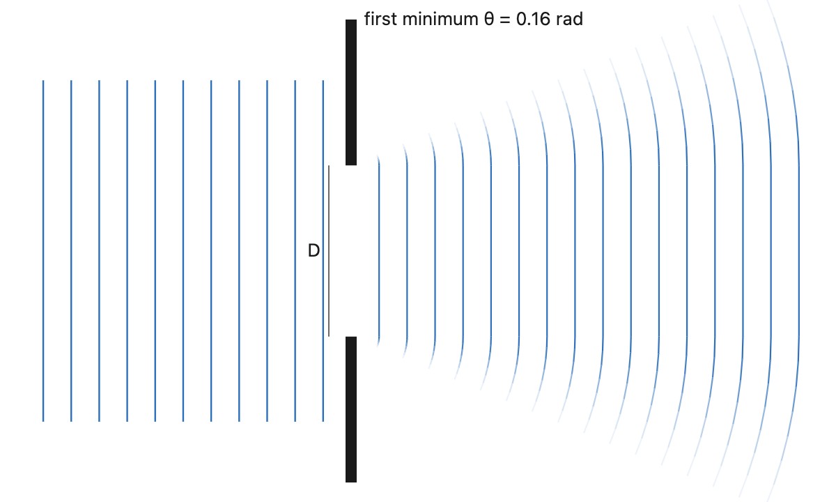
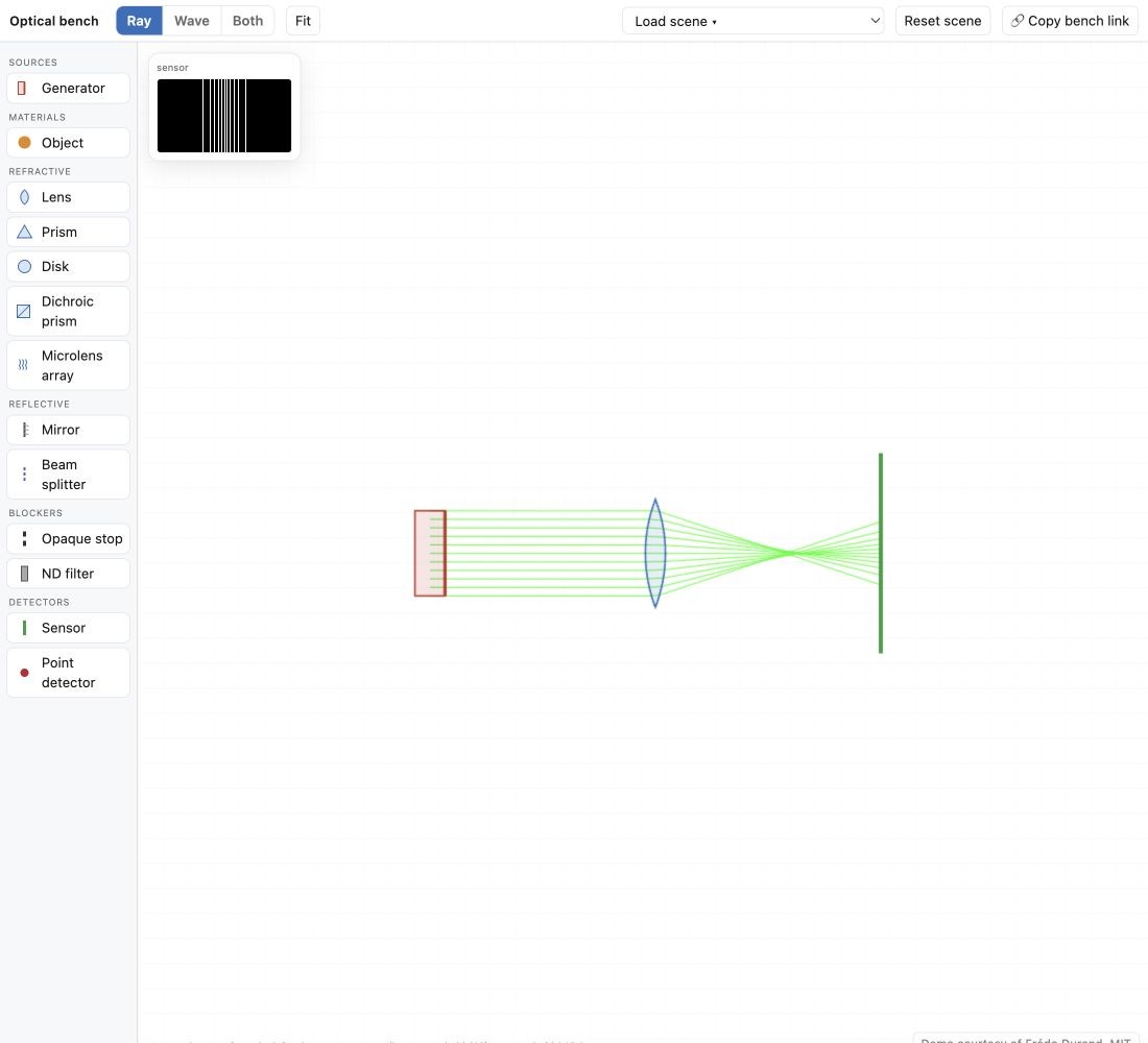
optionalThe wave picture imposes a limit on every imaging system ever made. When light passes through a small aperture or skims a sharp edge, it does not continue in perfectly straight rays: it diffracts, bending and spreading out. And, counterintuitively, the smaller the aperture, the more the light spreads (Figure 2.1.45). A wide opening lets the wavefront through almost undisturbed; a narrow one forces it to fan out, through an angle of roughly $\theta \approx \lambda / D$ for an aperture of diameter $D$.
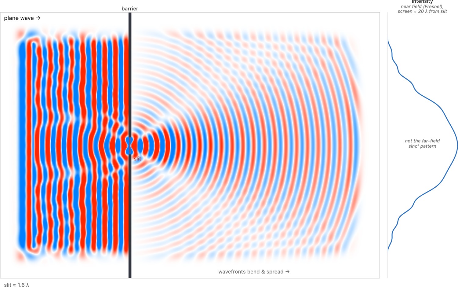
Where does that spreading come from? It is purely a property of waves, and we can watch it happen by solving the wave equation directly. Send a flat wavefront at an opaque barrier with a single slit and let the wave evolve in time: in front of the slit the wavefronts stay flat, but the moment they pass through, they bow into expanding circular arcs and fan outward (Figure 2.1.46). Narrow the slit relative to the wavelength and the fan opens wider: exactly the $\theta \approx \lambda / D$ behavior, now an emergent consequence of the wave dynamics rather than a rule asserted.
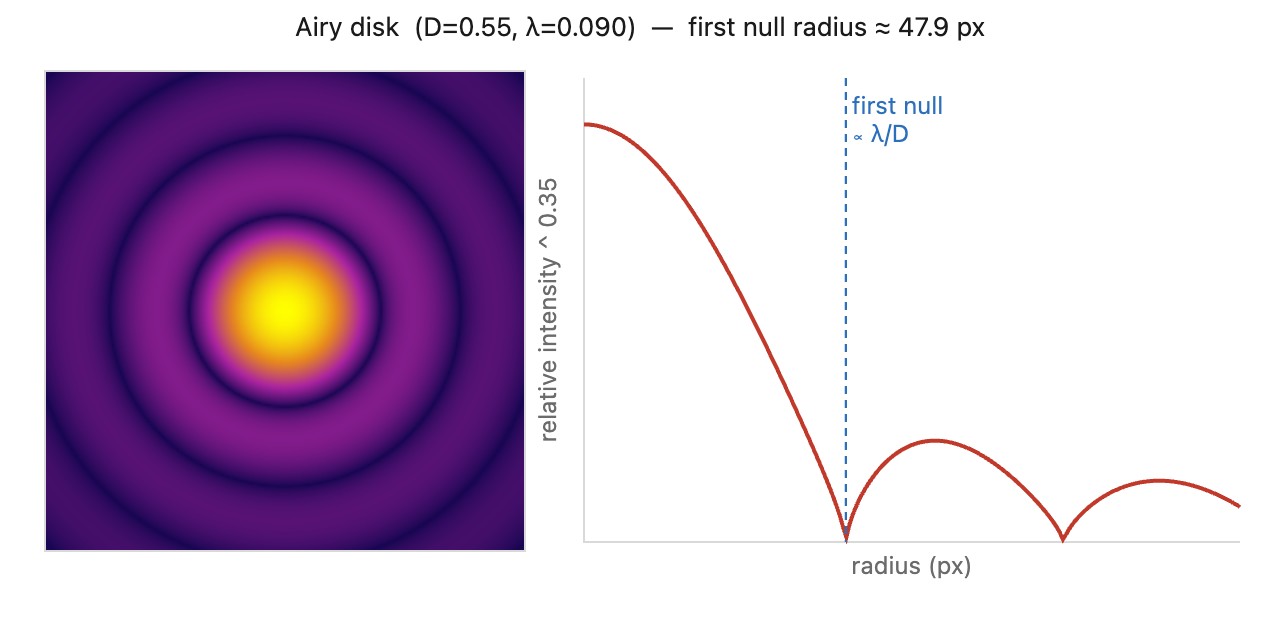
The Airy disk. The consequence for imaging is unavoidable: a finite aperture cannot focus light to a perfect point. Even a flawless, aberration-free lens images a single distant point not as a point but as a small bright blur, the Airy disk, surrounded by faint rings, whose angular radius is
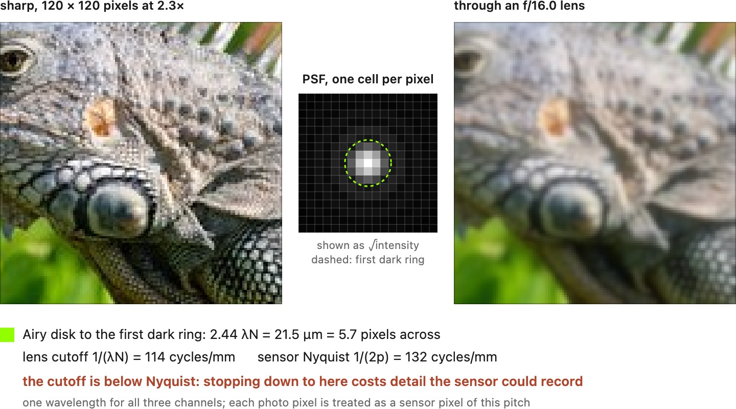
giving a blur-spot diameter on the order of $2.44\,\lambda N$, where $N = f/D$ is the lens's f-number (Figure 2.1.47). The Airy pattern describes an aberration-free, uniformly illuminated circular pupil in the scalar far-field model. Other pupil shapes or weightings change its central lobe and sidelobes; the quoted diameter measures the first dark ring, not the entire extent of the blur.
The diffraction limit. Because two nearby point sources blur into two overlapping Airy disks, there is a finest detail a lens can resolve: the diffraction limit. By the Rayleigh criterion, two points are just resolvable when the center of one Airy disk falls on the first dark ring of the other, again at $\theta \approx 1.22\,\lambda/D$. The headline is that a larger aperture diffracts less and resolves finer detail. It is worth putting numbers to that, because the limit is not an abstraction: it decides whether a given lens can read a license plate across a street or separate two stars (Figure 2.1.48).
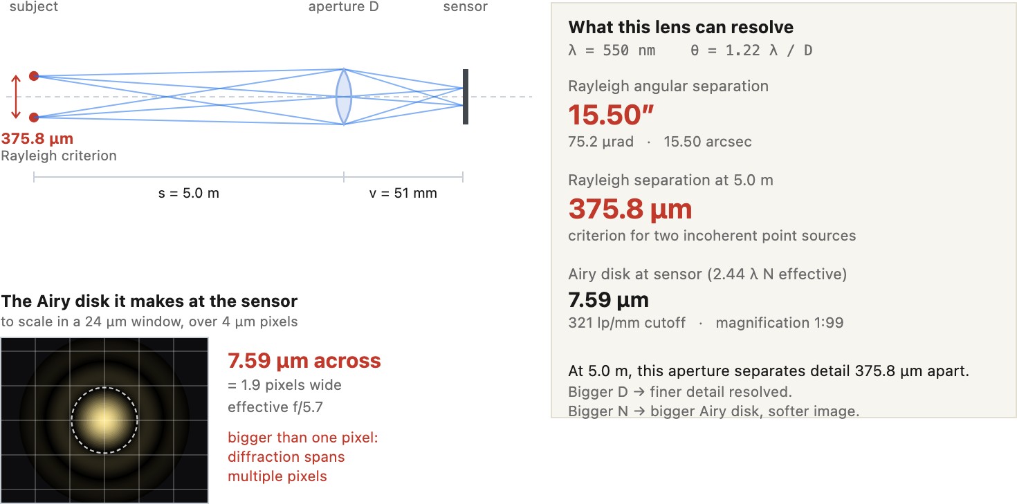
Counter to ray-optics intuition, a smaller aperture spreads light more: the diffraction blur (the Airy disk) grows as $\sim\!\lambda N$ with f-number, so stopping down past a point softens the image instead of sharpening it. The flip side is the rule behind every instrument that must resolve fine detail: only a large aperture can diffract little and resolve finely, which is exactly why microscopes and telescopes are built around large lenses and mirrors, and why a phone camera's tiny aperture hits a hard resolution wall it cannot pass. It is the optical cousin of "you can't sample your way past Nyquist."
This produces the photographer's sweet spot. Open the aperture wide and aberrations (the imperfections of real glass, deferred to the Optics part) dominate, softening the image. Stop the aperture far down and diffraction dominates, softening it again. Somewhere in between, typically a couple of stops down from wide open, the two effects are jointly minimized and the lens is at its sharpest. "Stopping down too far softens the image" is not a defect of cheap lenses; it is physics, and the trade-off is made quantitative with the modulation transfer function in the Optics part.
Motion blur⧉
Blur from subject motion⧉
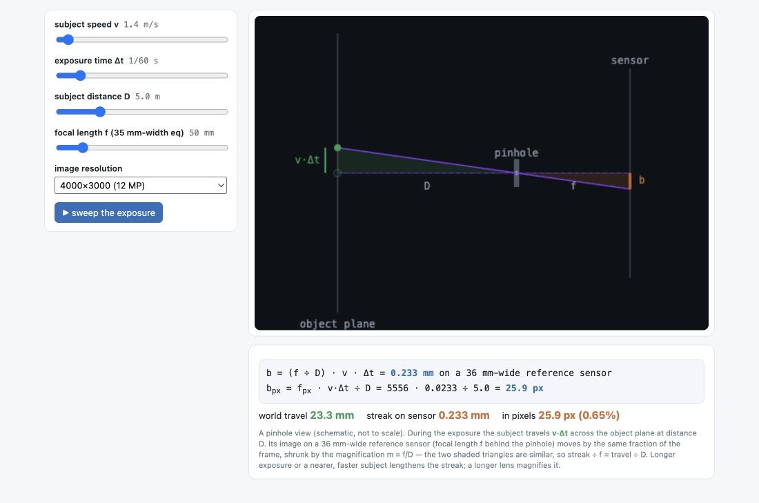
optionalTake an object moving with velocity $v$ (m/s) across the field of view (perpendicular to the optical axis), at distance $D$, imaged by a lens of focal length $f$. During the exposure $\Delta t$ it travels a world distance $v\,\Delta t$. The lens shrinks world distances at the subject plane by the magnification $m \approx f/D$ (for $D \gg f$), so the streak on the sensor has length
and in pixels, writing the focal length in pixels as $f_{\text{px}} = f/p$ with $p$ the pixel pitch,
The transverse component gives the simple streak above; motion straight toward or away from the camera rescales the object during the exposure, a radial blur of relative size about $\Delta z / D$, usually small for a distant subject and a short exposure but not for a close subject moving toward the lens. The result is a straight streak of that length as long as the velocity is roughly constant over $\Delta t$, which is the linearization we make: over the few milliseconds of a normal exposure, even curved or accelerating motion is well approximated by a straight segment. As a feel for the numbers, a person walking at $v = 1.4$ m/s at $D = 5$ m, shot at $50$ mm on a full-frame $24$-megapixel sensor ($f_{\text{px}} \approx 8300$) at $\Delta t = 1/60$ s, smears about $b_{\text{px}} \approx 40$ px: clearly visible, reduced to about $5$ px at $1/500$ s, which may still be visible at full resolution.
The derivation is one pair of similar triangles, which is easiest to see by moving the parts (Figure 2.6.1).
Blur from camera shake⧉
optionalNow hold the subject still and let the camera move during the exposure, which shifts the whole image at once. Hand tremor has two components, and they behave very differently.
The motions that cause shake are tiny, far below what the eye can follow, which is exactly why they are easy to underestimate. They can be made visible by motion magnification, which amplifies imperceptible sub-pixel movement in a video until it is plainly seen (the video below).
Translation. If the camera shifts sideways by $\Delta_c$ (perpendicular to the axis), it is exactly the subject-motion case with the roles swapped, applied to the entire scene:
Like subject motion, translational shake is depth-dependent: near objects blur more than far ones, and a distant background barely blurs at all. A shift along the axis by $\Delta_z$ gives a small radial "zoom" blur, $b_{\text{px}} \approx r\,\Delta_z/D$ at image radius $r$, normally tiny.
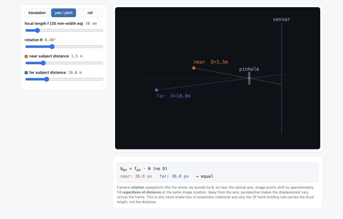
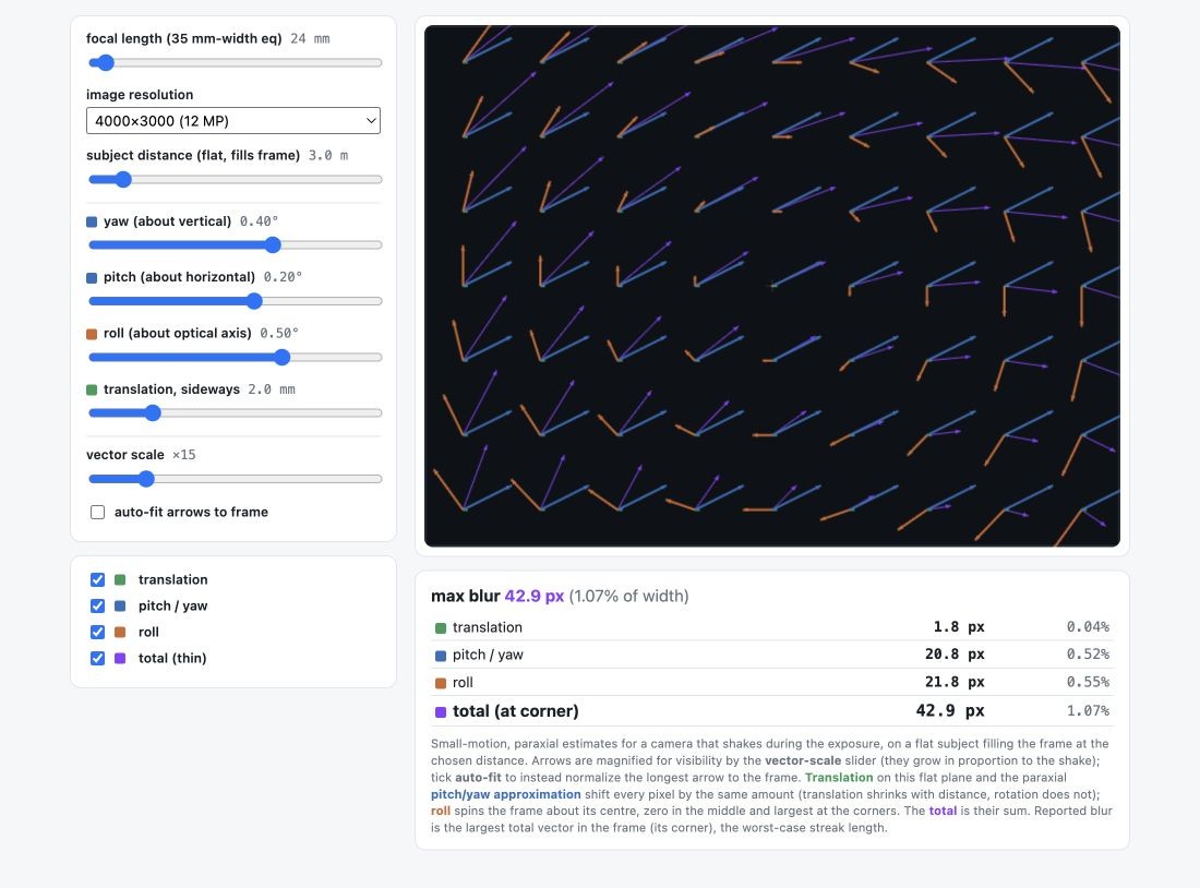
Rotation. If the camera instead rotates by a small angle $\theta$ (radians) about a horizontal axis (pitch) or vertical axis (yaw), the small-angle linearization $\tan\theta \approx \theta$ gives a whole-image shift of
Note what is absent: there is no $D$. Rotational blur is independent of the subject's distance: a rotation tilts the bundle of rays for near and far points by the same angle, but the pixel displacement can still vary with field position. Rotation about the optical axis (roll) instead spins the image about its center: a point at image radius $r$ (in pixels, measured from the center) moves by
zero at the center and growing toward the corners. Note the contrast with yaw and pitch: their blur carries the focal length $f_{\text{px}}$, so it is magnified by a longer lens, whereas roll carries only the image radius $r$, which is capped at half the frame no matter the focal length.
Camera rotation (yaw/pitch) smears the image by $b_{\text{px}} \approx f_{\text{px}}\,\theta$, the same for every object regardless of depth. Camera translation and subject motion smear it by $b_{\text{px}} \approx f_{\text{px}}\,(\Delta \text{ or } v\Delta t)/D$, which shrinks with distance. So for ordinary distances rotation dominates, and only up close (macro) does translation take over. The focal-length dependence divides the same way: yaw and pitch blur scale with $f_{\text{px}}$, so a longer lens (higher magnification) turns the same angular wobble into proportionally more blur (the basis of the $1/f$ hand-holding rule), while roll blur $b \approx r\,\theta_{\text{roll}}$ is fixed by image position $r$, not by focal length. Magnification amplifies yaw and pitch but never roll, which is why yaw and pitch usually dominate the shake blur, the more so the longer the lens. And because roll and perspective make $b$ vary across the frame, camera-shake blur is spatially non-uniform: a single blur kernel cannot describe or undo it.
The three shake terms read more clearly as geometry than as formulas (Figure 2.6.2), and add up on a real frame (Figure 2.6.3).
Preparing photographs for viewing⧉
Sharpening for the display: size and distance⧉
optionalApply output sharpening after resizing, and judge it at the intended size and viewing distance. A radius measured in pixels has a different angular scale on a small web image and a large print. A few source pixels can become less than one output pixel after reduction; choosing a radius on the final grid controls the edge neighborhood that will actually be displayed.
A useful workflow separates capture, creative, and output sharpening. Capture sharpening compensates for some capture softness within the information recorded by the lens and sensor. Creative sharpening directs attention to selected features, such as eyes or texture. Output sharpening compensates for the final presentation. They need not all be strong or even necessary. A phone JPEG may already contain substantial sharpening.
Paper and ink spread change edge contrast, so a matte print can require different settings from a glossy print or a screen. A distant poster can tolerate halos that would be objectionable in a handheld photograph. A 100% monitor view is useful for diagnosing artifacts, but it represents the final viewing situation only if its scale and distance match the output.
Inspect smooth skin, textured regions and a strong edge; the setting that makes one look crisp may damage another. Use a small test print to check whether fine contrast survives on the chosen medium. Repeated sharpening can exaggerate compression artifacts and produce bright and dark rims. Sharpening cannot restore an out-of-focus eye merely by strengthening its edges.
Reflected ambient light raises the visible black level. Prepare and judge the image under its intended viewing conditions; a panel specification alone does not describe the contrast the viewer will see.
Introduction to forward and inverse linear methods⧉
optionalA blurred edge spreads a sharp transition across several pixels. If we know how that spreading happened, can we recover the edge? A short row of samples is enough to show both the calculation and its limits.
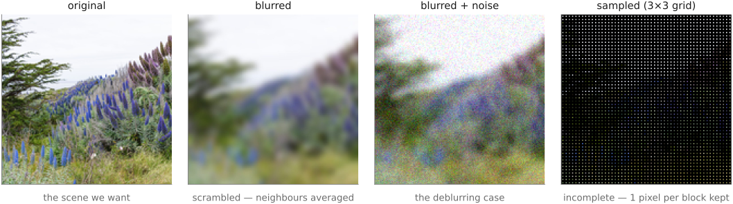
The forward problem predicts a measurement from a scene and a camera model. The inverse problem estimates the scene from the measurement. We will use a known linear model; learning an unknown blur or geometry is an additional estimation problem. Deblurring, denoising, demosaicking, and super-resolution differ in what was measured and what assumptions recovery needs.
We compare a blur, an idealized corner camera, and a sampling grid. A blur attenuates detail and may erase some patterns entirely. A corner camera records a weak indirect signal. A coarse sampling grid cannot distinguish arbitrary fine patterns. These examples separate noise sensitivity from non-uniqueness.
An operation $F$ is linear when $F(a x+b x')=aF(x)+bF(x')$. For finite sampled signals, each output is a weighted sum of inputs with weights independent of the data. Stacking those weights into rows gives $y=Ax$. The matrix describes the operation; code can apply its weights without allocating the matrix.
A one-dimensional blur, forward⧉
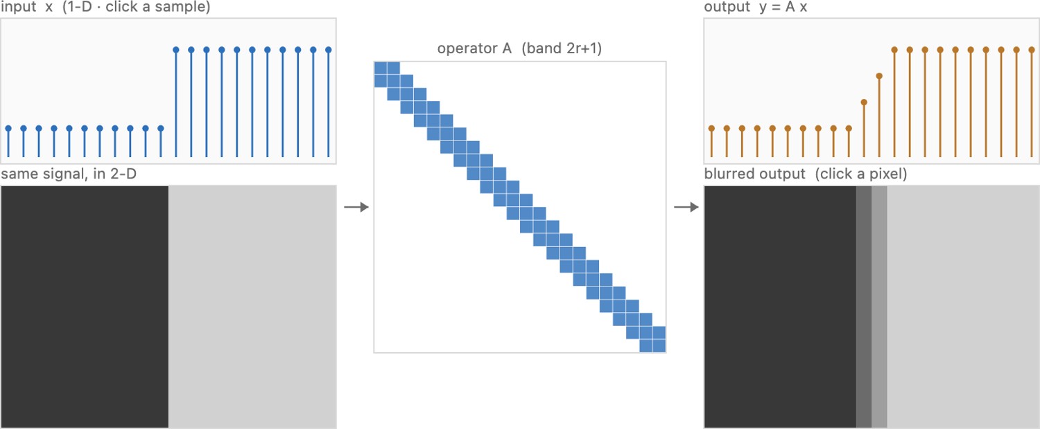
optionalStrip the image down to a single row of pixels, a one-dimensional signal $x = (x_1, x_2, \dots, x_n)$. Think of it as one scanline of a photo, or a flat 1-D world. Now blur it in the gentlest possible way: replace every sample by the average of itself and its two immediate neighbors. This is the box blur of radius one,
Each output sample is a little local average, so sharp features soften and fine wiggles wash out, which is exactly what optical blur does to a real photo (the full two-dimensional story is Chapter 6.2, Convolution).
Now write the same operation as a single matrix multiply. Stack the outputs into a vector $y$, collect the averaging weights into a matrix $A$ with one row per output sample, and the blur becomes
For a five-sample signal, with the edges handled by repeating the end pixel, the matrix is small enough to print in full:
Row three gives $y_3=(x_2+x_3+x_4)/3$. The repeated interior weights make a narrow band, while the first and last rows encode the chosen boundary rule. Other cameras need not have this banded structure.
This is the forward model: hand it a scene $x$, and it returns the measurement $y$. Computing it is trivial, a few multiplies and adds per sample, or in code a single loop:
# forward: 1-D box blur of radius 1, edges replicate
for i in range(n):
    y[i] = (x[clamp(i-1, 0, n-1)] + x[i] + x[clamp(i+1, 0, n-1)]) / 3
Convolution⧉
PS2 implements box/Gaussian blur, gradients, sharpening, and the bilateral filter. → Chapter 1.5, Problem sets (appendix).
A blur softens an edge by mixing neighboring values. A derivative measures their differences, and a sharpener adds some of those differences back. All three can use one table of weights applied throughout the image, a convolution kernel.
Blurring is useful before downsampling, for noise reduction, and for building image pyramids. It also models some optical degradation. A single kernel is appropriate only when the point spread is the same across the region being modeled; depth changes and camera motion often require a more general operator.
Sharpening increases local contrast. It can make surviving detail easier to see, but it is not generally the inverse of the blur that formed an image.
Convolution as a weighted sum of neighboring pixels⧉
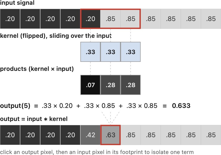
A kernel assigns a weight to each displacement between an input and an output sample. Nonnegative weights summing to one form a local average. Derivative and sharpening kernels can have negative weights, so convolution is more general than averaging.
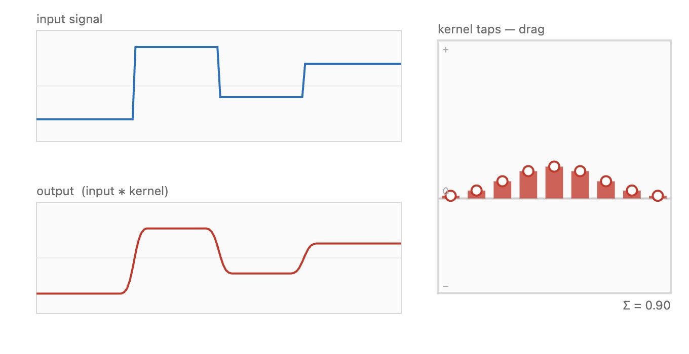
It is easiest to see in one dimension first (Figure 6.2.1), where the whole operation is a 3-tap kernel sliding along a row of pixels: each output pixel is the weighted sum of the three input pixels under the kernel, and nothing more.
The two-dimensional case is the same thing with a small grid of weights instead of a row (Figure 6.2.2).
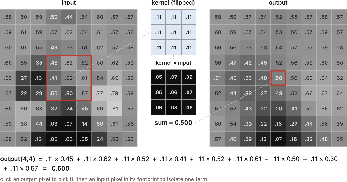
Two properties of this scheme are important. First, it is linear: each output pixel is a weighted sum of input values with fixed weights, so scaling the input scales the output, and adding two images adds their outputs. Second, it is shift-invariant: the same kernel applies at every pixel, so the operation does not care where in the image you are. Formally, writing $S_d$ for a shift by $d$ pixels, a shift-invariant operation commutes with shifting, $F(S_d\,x) = S_d\,F(x)$: shift the input and the output just shifts to match. Such an operation is linear and shift-invariant (LSI). This characterization assumes an infinite grid or compatible periodic boundaries; finite-image extensions require separate attention below.
Both conditions are real constraints, and it helps to watch one break. A graduated neutral-density filter (the kind that darkens the sky at the top of the frame while leaving the foreground alone) multiplies each pixel by a factor that depends on its row, say $(1 - y/y_\max)$. That is still linear (scaling the input scales the output), but it is emphatically not shift-invariant: slide the image down and the darkening falls on different content. So it is a linear operation that is not a convolution. Convolution is the well-behaved special case where the rule is identical everywhere, and that uniformity is exactly what later lets the Fourier transform pry it open.
A convolution uses fixed weights that depend on displacement, not on image values or absolute position. On an infinite or periodic grid it is linear and commutes with shifts. The kernel can be small or span the image. Its support determines the work of direct filtering; finite boundaries determine where the shift-invariance model applies.
Defocus varies with scene depth, camera rotation produces position-dependent image motion, and aberrations can vary across the field. These effects may remain linear in scene intensity for fixed geometry while requiring different point-spread functions at different locations. A nearly constant PSF over a small patch can justify a local convolution. At depth or motion boundaries, occlusion can invalidate that approximation. Chapter 6.7, Image formation as a linear system treats general operators and Chapter 16.4, Blind deblurring develops camera-motion models.
A linear model lets us study which patterns a measurement preserves and which it attenuates. Physical mixing must act on linear-light values. Filtering encoded values is a different operation, even when the same arithmetic is used; Chapter 4.3, Encoding: linear, gamma or log explains the distinction.
The algorithm itself is a short loop. Zero the output, then for every output pixel, walk over the kernel, multiply each input neighbor by its weight, and accumulate:
for each output pixel (x, y):
    out[x, y] = 0
    for each kernel offset (x', y'):
        out[x, y] += in[x + x', y + y'] · g[-x', -y']
assuming the kernel's coordinates are centered on zero. The minus signs on the kernel coordinates are the flip: each input neighbor is multiplied not by the weight at its own offset but by the weight at the opposite one. That flip is exactly what separates convolution from correlation, and why it matters is the subject of the next section.
The flip: where-from vs. where-to⧉
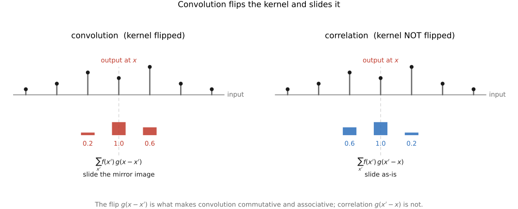
The minus signs in the loop above, the kernel read at g[-x', -y'] rather than g[x', y'], are the flip. The textbook definition writes the same operation by subtracting the offset on the kernel:
In words: to get the output at $x$, sum over all input positions $x'$, each weighted by the kernel evaluated at $x - x'$, the kernel is flipped (and slid) before it is multiplied in. Why the flip, and does it matter?
The flip is the difference between where light goes to and where light comes from. The physical, forward model says light at scene position $x$ lands, blurred, at sensor positions $x + x'$ for the offsets in the kernel; light spreads outward. But when we compute the output at a fixed pixel $x$, we are asking the backward question: which input pixels contributed here? The answer is the ones at $x - x'$. The minus sign is nothing but the bookkeeping of inverting "where-to" into "where-from."
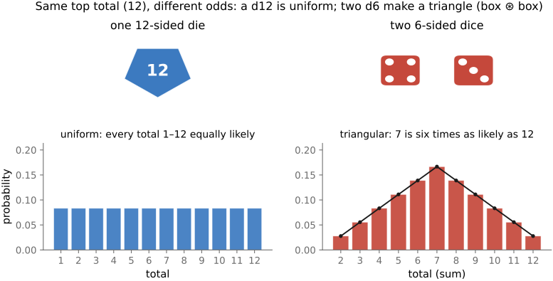
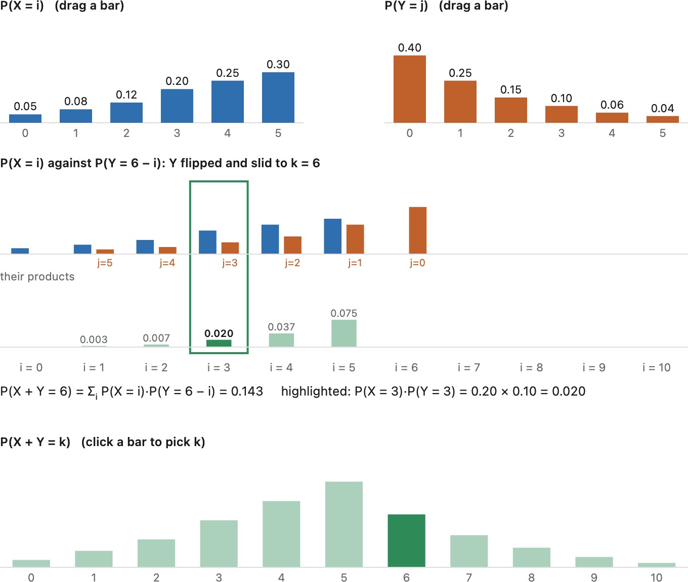
If $X$ and $Y$ are independent with known distributions, the distribution of $X + Y$ is their convolution, and the flip falls out for free. To ask "how likely is $X + Y = x$?", enumerate the ways it can happen: $X = x'$ paired with $Y = x - x'$, for every $x'$. The second variable is forced to be the sum minus the first, and you add up the products of probabilities over all $x'$. That $x - x'$ is exactly the convolution flip, here not a convention but a logical necessity. The cleanest instance is two dice: each die is a flat distribution over 1–6 (a one-dimensional box), and the distribution of the total is that box convolved with itself, a triangle peaking at 7 (Figure 6.2.5). This is why, throwing two dice, a sum of 7 is much more likely than a 12: there are six ways to roll a 7 (1+6, 2+5, 3+4, 4+3, 5+2, 6+1) but only one way to roll a 12 (6+6), so a 7 comes up six times as often, the middling totals win because there are simply more ways to reach them. A box convolved with a box is a triangle; the box returns in the blur zoo.
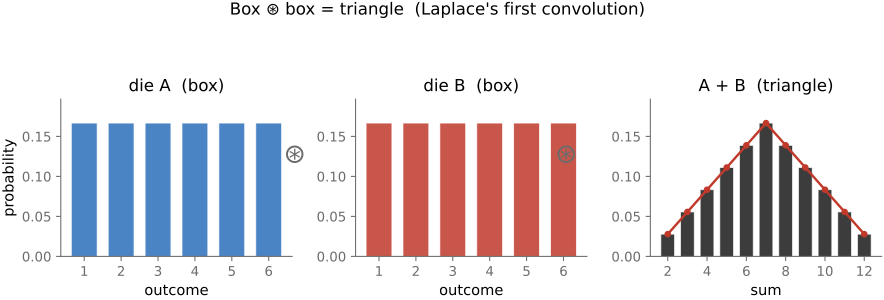
The same point is easy to miss with real dice. A single twelve-sided die and a pair of six-sided dice both top out at a total of twelve, yet they are nothing alike: the d12 is uniform (every total equally likely), while two d6 make a triangle, because their sum is a box convolved with a box (Figure 6.2.6).
For a symmetric kernel, convolution and real-valued correlation agree. For an asymmetric kernel, omitting the flip changes the operation; a derivative may reverse sign and a shift may reverse direction. Correlation is useful for matching a template against an image. State which convention the code uses rather than inferring it from a function name.
Test the convention with an asymmetric kernel rather than a Gaussian. A kernel with one nonzero tap displaced from its center should shift a single bright pixel in a predictable direction. Flipping the kernel reverses that direction. With a finite-difference kernel, the sign of a rising step distinguishes the two conventions. A symmetric blur cannot expose the mistake because it is unchanged by the flip. This is why a filter test suite needs a directional example even when the application mainly uses symmetric kernels.
A convolutional neural network does not flip. A "convolution" layer computes the correlation of its input with a learned kernel, which is what almost every deep-learning framework implements under that name. Nothing is lost by it: the kernel is fitted to data, so whichever orientation the layer needs, training finds it, and a flipped kernel is just as learnable as its mirror. The name is inherited from signal processing rather than earned. The distinction comes back in two places. One is at the boundary with classical code, where a kernel taken from a paper or from a library that does flip has to be flipped to match. The other is in the backward pass: the gradient of a correlation with respect to its input is a convolution, which is where the transposed convolution used in decoders and upsampling layers comes from. Chapter 7.3, Deep learning develops the layers themselves.
Convolution as a sum of translated images⧉
optionalEverything so far has read convolution locally: fix an output pixel and gather a weighted sum of its neighbors. The same operation has a second, global reading. Instead of building the output one pixel at a time, build it one kernel tap at a time: each tap takes the whole input image, shifts it, scales it by the tap's weight, and adds it into the running total. Read this way, the output is a weighted sum of translated copies of the input, one copy per kernel tap.
The two readings are the very same double loop, only nested in the opposite order. Both zero the output, then run over every (output pixel, kernel offset) pair and add in[x + x', y + y'] · g[-x', -y'] each time. The one change is which for each line is the outer one; the body is identical. Coloring the output-pixel loop (blue) and the kernel-offset loop (red) makes the swap plain:
Local, the output-pixel loop on the outside:
out ← 0
for each output pixel (x, y):
    for each kernel offset (x', y'):
        out[x, y] += in[x + x', y + y'] · g[-x', -y']
Global, the kernel-offset loop on the outside:
out ← 0
for each kernel offset (x', y'):
    for each output pixel (x, y):
        out[x, y] += in[x + x', y + y'] · g[-x', -y']
In the local version the inner loop assembles one output pixel from all the taps; in the global version each pass of the outer loop adds one scaled, translated copy of the whole input, so the output grows as a sum of shifted images, $\text{out} = \sum_{x', y'} g[-x', -y']\,\cdot\,\text{shift}(\text{in},(x', y'))$. Same result, accounted from opposite ends. But the global reading buys three things the local one hides.
A fixed weighted sum of warped images is still linear in image intensity when the warps and interpolation weights are fixed. Pure camera rotation produces projective warps (homographies); roll alone is an in-plane rotation. Replacing shifts with these warps models motion that a single convolution cannot capture. Translation through a scene with varying depth also requires depth and visibility.
The global form also explains Fourier analysis: a complex exponential is multiplied by a scalar under each shift, so a weighted sum of shifts multiplies it by the weighted sum of those scalars. Chapter 6.3, Fourier develops this frequency response.
Translations commute on an infinite or periodic grid, so their weighted sum commutes with translation. Cropping or re-extending a finite image between operations can break this algebra.
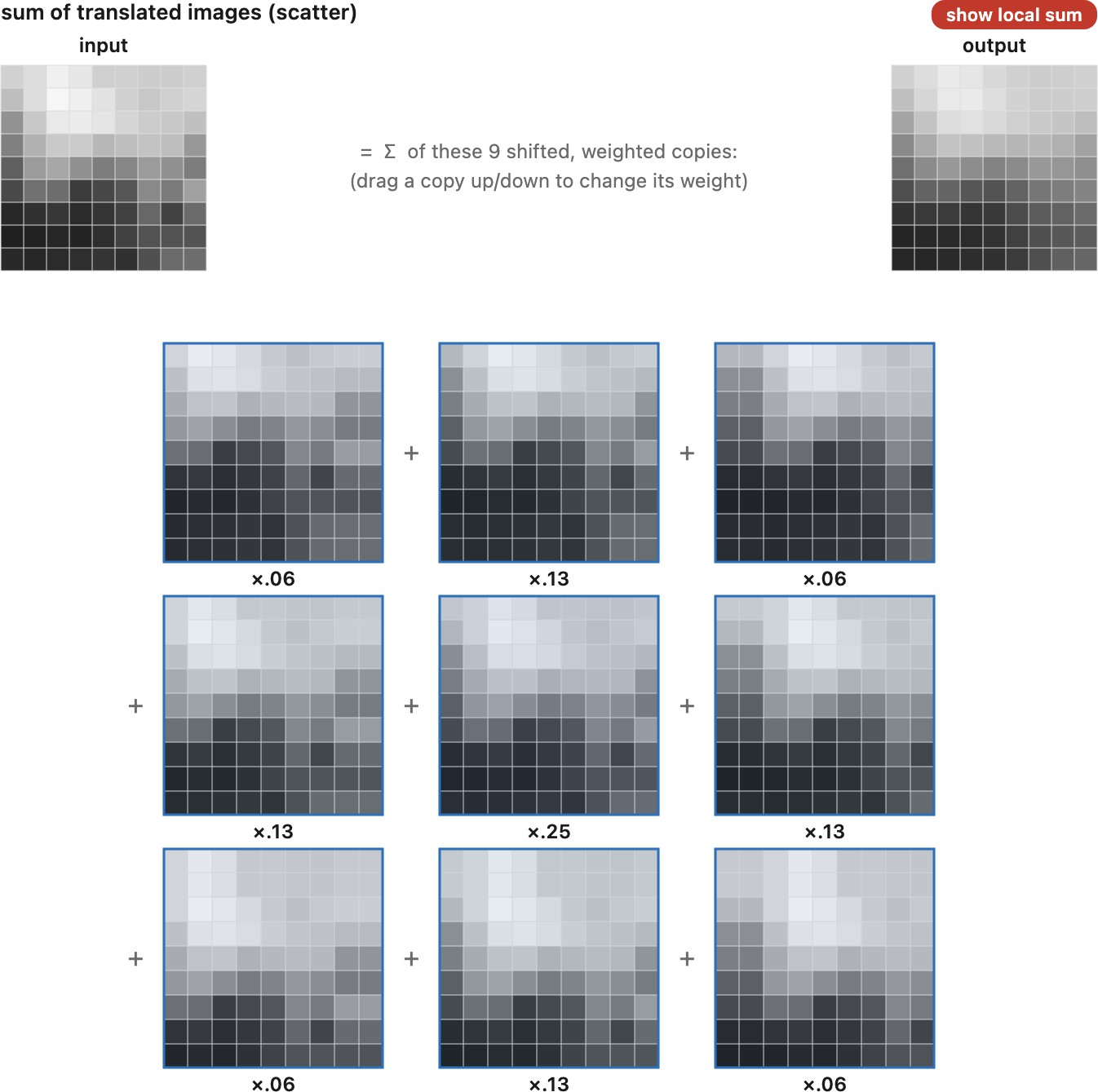
Convolution can be computed per output pixel or per kernel tap. In the first order we accumulate a neighborhood; in the second we accumulate shifted copies of the image. The result is the same. Replacing shifts with known warps gives other linear operators, but they need not share convolution’s commutativity or Fourier diagonalization.
Properties: the impulse, normalization, symmetry, commutativity⧉
A handful of properties make convolution pleasant to work with, and the slickest way to expose them is to feed the filter the simplest possible input: one bright pixel on a black background, the impulse $\delta$ (the discrete Dirac / Kronecker delta, one at the origin, zero everywhere else).
Convolve an impulse with a kernel and you get the kernel back, stamped at the impulse's location. The flip explains why: every output pixel asks "where did my light come from?", and the only nonzero input is the single bright pixel, so each output simply picks up the kernel weight that connects it to that pixel, tracing out the kernel. This output carries a name borrowed from optics: the point spread function (PSF), or impulse response. It is literally how the system spreads a single point of light, the very blob you saw around the streetlight. So the kernel, the impulse response, and the PSF are three names for one thing, with an immediate practical corollary: to discover what a filter does, feed it an impulse and read off the kernel. This is the single best debugging input for convolution code, and we will lean on it.
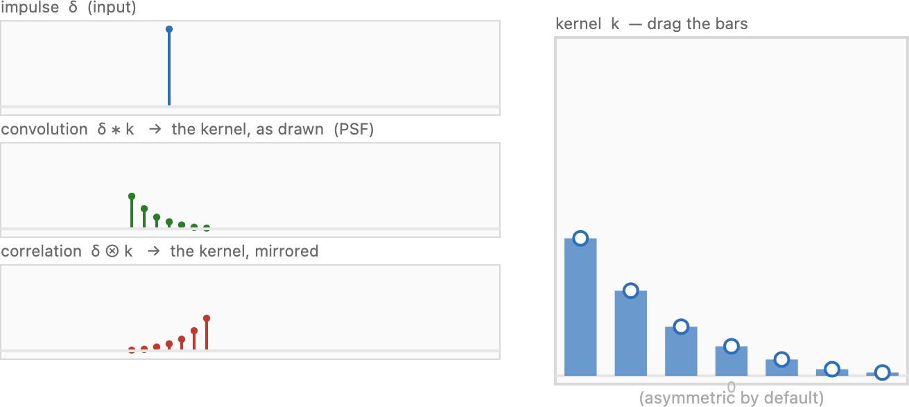
Convolve an interior impulse with an asymmetric kernel: the output should reproduce that kernel in its declared offset coordinates, not its flipped version. A constant tests unit-sum weights only where the boundary extension also preserves constants. A single nonzero off-center tap tests shift direction. A ramp tests derivative sign and scale, and an edge tests the step response. Start in one dimension and calculate a few outputs by hand. See Figure 6.2.9.
A straight step edge gives another measurement. Under locally shift-invariant blur, differentiating its edge-spread function gives the line-spread function, the PSF integrated along the edge direction. One edge orientation gives one projection, not the full two-dimensional PSF. A natural edge also includes its original softness, texture, noise, and earlier processing; controlled slanted-edge targets are used for quantitative MTF measurement.
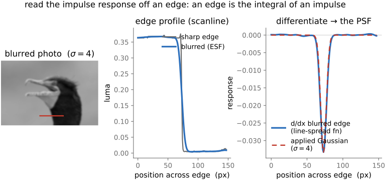
The identity element follows at once: convolving with the impulse leaves the image untouched, $I * \delta = I$, because reading "where-from" with a kernel that points only at yourself just copies you. The remaining properties:
- Normalization: weights summing to one preserve a constant signal when the boundary rule preserves that constant. This is not a guarantee that every finite crop preserves total energy. Derivative weights sum to zero; do not normalize them to one.
- Commutativity and associativity: on the full domain, $I*g=g*I$ and $(I*g)*h=I*(g*h)$. Consistent circular convolution has the same properties. Cropping and applying a fresh boundary extension after each pass can change the result.
- Linearity and shift-invariance together give the Fourier representation. Linearity alone does not make an operator diagonal in Fourier coordinates.
Nitty-gritty: finite images⧉
Two practical wrinkles before the kernels themselves.
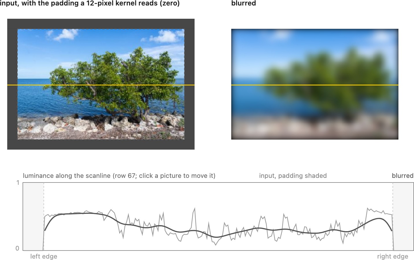
First, the kernel must be centered. Our images place $(0, 0)$ at the top-left corner, but a blur kernel is naturally centered on the pixel it is computing, its weights run from $-r$ to $+r$ around the middle, where $r$ is the kernel radius, so the full size is $(2r+1) \times (2r+1)$. An off-by-one here shifts the whole image by a pixel; an impulse test catches it instantly, because the blob lands off-center.
A finite image needs an extension rule: zero, repeated edge values, reflection, or periodic wrapping. Zero padding darkens a blurred border; reflection and clamping preserve constants but make different assumptions about missing content. Reflection conventions also differ in whether the edge sample is repeated. Use one declared convention in both the model and the implementation. Allocate a separate output buffer so earlier writes do not alter later inputs.
For a finite operator $A$, its transpose must reverse both filtering and boundary handling. A symmetric kernel does not by itself make a clamped or reflected implementation self-adjoint. This distinction matters when the filter appears inside an inverse solver.
A blur zoo⧉
With the mechanics settled, the only choice left is the kernel's shape. Two are worth knowing.
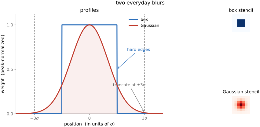
The box filter gives every sample in a $(2r+1)\times(2r+1)$ window weight $1/(2r+1)^2$. Its square footprint is not rotationally symmetric, and its frequency response has lobes and zeros. However, its nonnegative weights cannot create overshoot beyond the neighborhood’s range; a blurred step becomes a ramp, not a ringing edge. Running sums can make large box averages inexpensive.
The Gaussian is the workhorse. Its weights fall off smoothly with distance from the center, following the bell curve
where $r$ is the distance to the center and $\sigma$ (the standard deviation) sets the width, the blur's "radius" in spirit. Read it back: a neighbor's weight decays exponentially with the square of its distance, so nearby pixels count for a lot and far ones fade smoothly to nothing. The Gaussian is smooth, rotationally symmetric (no directional bias), and, as the next chapter shows, uniquely well-behaved in frequency, which is why it is the default blur almost everywhere.
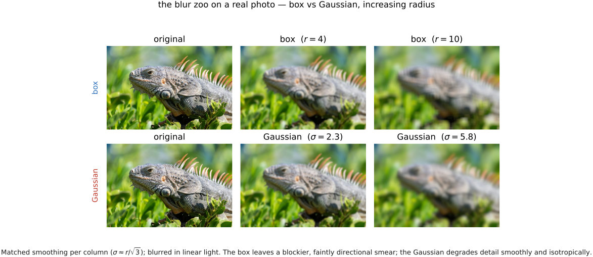
Run both on an actual photograph and the difference in feel is plain: the box smears fine texture into faintly blocky, slightly directional mush, while the Gaussian dissolves it smoothly and isotropically. Use a Gaussian when the blur should look natural (Figure 6.2.13).
Better than reading about them, you can try the blurs directly (Figure 6.2.14): switch kernels, change the width, and watch what each does to real texture.
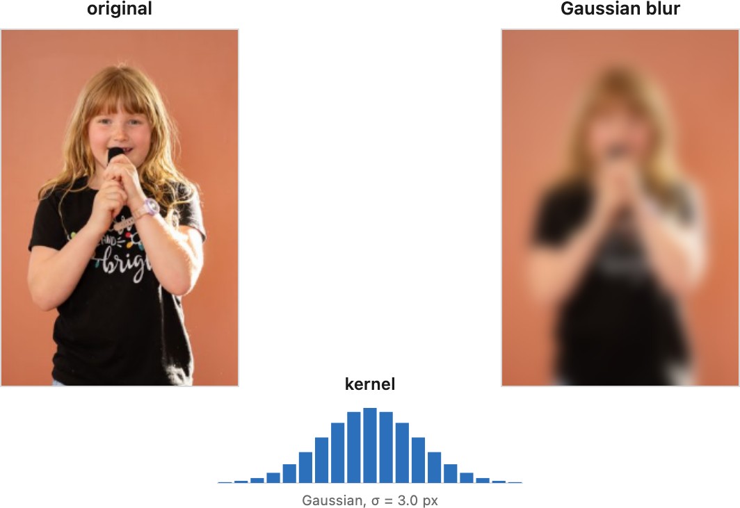
An ideal Gaussian has infinite support. At a distance $3\sigma$, its weight is $e^{-9/2}\approx0.011$ of the peak; a one-dimensional cut at $\pm3\sigma$ discards about 0.27% of the mass. Choose support for the required accuracy and renormalize the sampled, truncated weights. Square truncation preserves separability; circular truncation generally does not. Sampling and truncation make rotational symmetry approximate.
To simulate physical mixing, decode to linear light, filter, then encode for display. Aesthetic smoothing can deliberately use another space, but it should be named. Linear-light processing is essential when the blur is part of a calibrated forward model. For images with transparency, filter premultiplied color and alpha consistently to avoid color bleeding from transparent pixels.
The visible encoding error is easiest to see where black meets white. Averaging their encoded values gives a middle code value; decoding that value generally yields less light than averaging the original linear intensities. A blurred highlight can therefore acquire a dark transition when filtering is done in the display encoding. The arithmetic is still linear in the stored numbers, but it no longer represents linear mixing of light.
Separability⧉
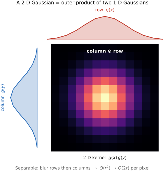
A $(2r+1) \times (2r+1)$ Gaussian appears to cost $(2r+1)^2$ multiplies per output pixel, quadratic in the radius, which is painful for a big blur. There is a shortcut. A 2-D filter is separable if it can be written as one 1-D filter applied along the rows followed by another along the columns, formally, the 2-D kernel is the outer product of two 1-D kernels. The Gaussian is separable, because $\exp(-(x^2 + y^2)/2\sigma^2) = \exp(-x^2/2\sigma^2) \cdot \exp(-y^2/2\sigma^2)$: a 2-D Gaussian is a horizontal 1-D Gaussian times a vertical one.
This is a genuine speedup. Instead of one $(2r+1)^2$ pass you do two $(2r+1)$ passes: blur every row with a 1-D Gaussian, then blur every column. The cost per pixel drops from $O(r^2)$ to $O(2r)$, linear in the radius. For a $\sigma = 10$ Gaussian (radius 30, a 61×61 kernel) that is the difference between ~3700 multiplies per pixel and ~120, about 30 times fewer multiplications, before accounting for memory traffic and implementation overhead. Separability is the first of several "do it in 1-D twice" tricks that recur through the book.
In code it is just two 1-D convolution passes with a scratch buffer between them:
# separable 2-D convolution: g = g_row ⊗ g_col, each 1-D and centered on zero
# pass 1: convolve every row with g_row
for each pixel (x, y):
    tmp[x, y] = 0
    for each offset x':
        tmp[x, y] += in[x + x', y] · g_row[-x']
# pass 2: convolve every column of the result with g_col
for each pixel (x, y):
    out[x, y] = 0
    for each offset y':
        out[x, y] += tmp[x, y + y'] · g_col[-y']
The box blur is separable in exactly the same way: an $n \times n$ average is an $n$-wide average along the rows followed by an $n$-wide average along the columns, so it too drops from $O(r^2)$ to $O(2r)$. Separability is a special property, though, not a universal one. A kernel factors like this only when it is rank one, its grid of weights being the outer product of a single row and a single column; a general kernel is not. The disk-shaped blur of a defocused lens is not separable, and neither is a diagonal motion streak, so those need the full 2-D sum or a different fast route (often the Fourier transform of the next chapter).
Linear sharpening⧉
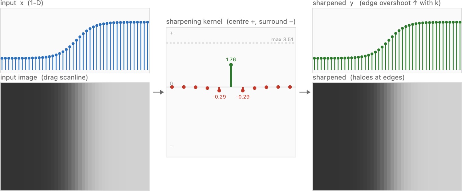
Blur mixes a pixel with its neighbors; sharpening does the opposite, making each pixel more different from its neighbors. Where the image is flat the neighbors agree and there is nothing to do; where a pixel stands out, at an edge or a fine texture, sharpening exaggerates the difference so the feature reads crisper.
There is an equivalent way to say it that ties straight back to blur. A blurred copy of an image is its smooth, low-detail part, so whatever the blur removed is exactly the fine detail: $\text{detail} = \text{in} - g * \text{in}$. Sharpening is amplifying that detail, putting it back with a gain $k$:
This is the unsharp mask, and because every piece is linear it collapses to a single convolution,
a kernel with a tall positive spike at the center (the identity $\delta$) minus a scaled blur around it: positive in the middle, negative in the surround. For a unit-sum blur, this kernel also sums to one and preserves a constant.
They form a small family, differing only in the blur $g$ (equivalently, the band of detail) they amplify:
- Unsharp mask. Take $g$ a Gaussian; $\text{in} - g*\text{in}$ is a high-pass, everything finer than the Gaussian, and its radius ($\sigma$) and amount ($k$) are the two sliders every photo editor exposes.
- Laplacian. At a one-pixel radius the classic sharpening kernel is a $+5$ center with four $-1$ neighbors (the identity minus the discrete Laplacian): the same idea at the smallest scale.
- Difference of Gaussians (DoG). Rather than one blur, subtract a wider Gaussian from a narrower one, $\text{DoG} = G_{\sigma_1} - G_{\sigma_2}$ with $\sigma_1 < \sigma_2$. This is a band-pass: it isolates one band of detail (features near a chosen scale) instead of all detail at once, so a DoG can boost medium-scale texture without amplifying the finest pixel noise. For nearby scales, a suitably scaled DoG approximates a Laplacian-of-Gaussian up to sign. It also supplies a simple model of center-surround responses and a filter for blob detection.
Sharpening with a DoG is then just
Because all of these are linear convolutions they inherit this chapter's machinery, separability included (each Gaussian factors into a row pass and a column pass). Two failure modes limit linear sharpening: it amplifies noise along with detail (noise lives in the same high band), and it overshoots strong edges into bright and dark halos. Curing those needs the nonlinear, edge-aware sharpening of Chapter 8.8, Sharpening.
Gradient and oriented filters⧉
optionalNot every useful kernel blurs. The most important non-blurring kernel measures change (how fast the image brightens or darkens as you step across it) and that turns out to be the foundation of edge detection.
With pixel spacing $h$, a forward difference is $I_x[i]=(I[i+1]-I[i])/h$. The weights $[-1,+1]/h$ act as a correlation stencil at offsets $0,1$. Under this chapter’s convolution convention, the same operation has $g[-1]=1/h$ and $g[0]=-1/h$. State the offsets as well as the weights: a two-tap stencil has no central sample. A ramp increasing to the right must produce a positive derivative.
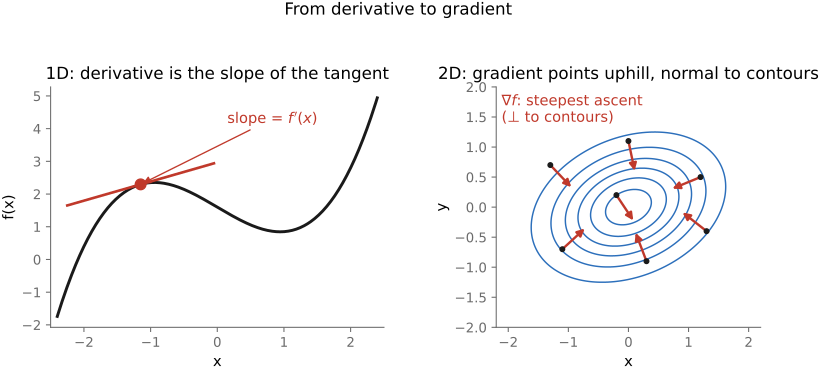
A grayscale image is a two-dimensional function (a brightness landscape with hills and valleys) so its derivative is not a single number but a gradient: a vector that, like the slope of a hill, points in the direction of steepest brightening and is perpendicular to the contours of constant brightness (Figure 6.2.17, right). Its two components are exactly the horizontal and vertical partials, $I_x$ and $I_y$, which is why we estimate each with its own finite-difference kernel.
Finite differences are convolutions with signed kernels under a declared indexing convention. In the continuous setting, $\partial_x(g*I)=(\partial_x g)*I$: convolving with a derivative-of-Gaussian differentiates a smoothed image. Gradient components are linear; gradient magnitude, thresholding, and a complete edge detector generally are not.
Differencing increases the contribution of rapidly varying noise. Sobel combines a difference along one axis with smoothing along the other. The following displayed matrix is a correlation stencil, using image coordinates with $x$ rightward and $y$ downward:
Divide its response by $8h$ to estimate a derivative in intensity per unit distance on a linear ramp. For convolution, flip the displayed stencil, which negates it. Its transpose gives the vertical stencil under the same convention.
The smoothing is what Sobel buys. Scaled by 1/4, it gives a step edge the same height of response as the plain difference $[-1,\,1]$, but it averages three rows, weighted 1, 2, 1, before differencing. On independent pixel noise of standard deviation $s$, the plain difference has noise $\sqrt2\,s$ and the scaled Sobel $\sqrt{12}/4\,s\approx0.87\,s$, about 1.6 times less. The price is resolution: Sobel's response to an edge is two pixels wide (Figure 6.2.18).
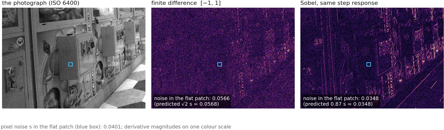
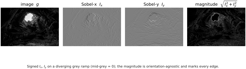
Stacking the two partials into a vector gives the image gradient $\nabla I = (I_x, I_y)$, the brightness-landscape gradient of Figure 6.2.17 applied to a real image. Two numbers fall out of it, both central to vision:
The magnitude is large at strong intensity changes, which can be object boundaries, texture, or noise. The gradient angle points across an edge; its tangent is perpendicular, $\theta+\pi/2$ modulo $\pi$. Thresholding magnitude gives a simple detector. Canny adds smoothing, non-maximum suppression, and hysteresis.
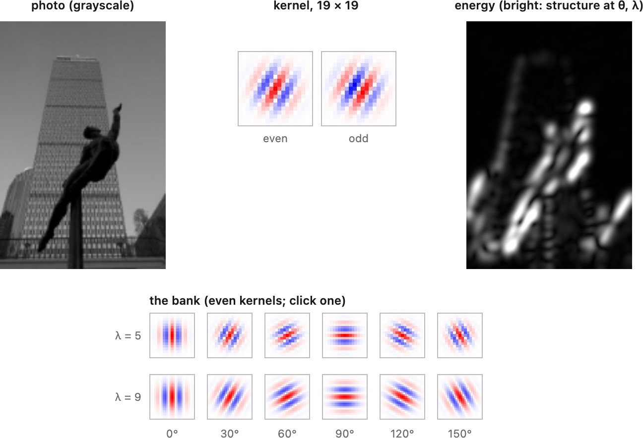
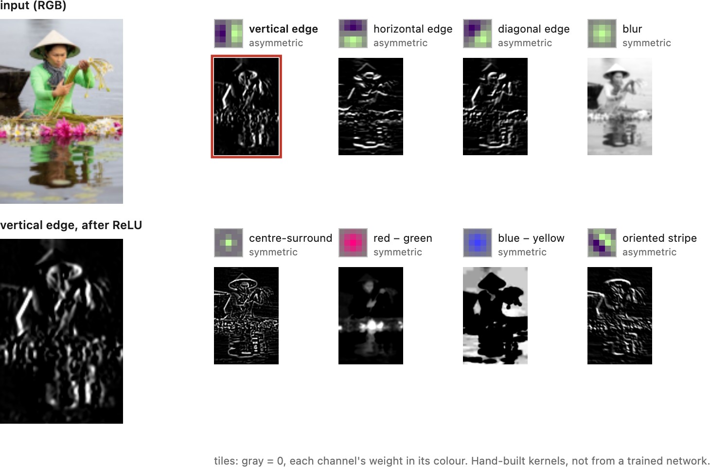
Blur, gradients, and sharpening all share the same comfortable assumption: one kernel, applied the same way everywhere. Before we lean on it, ask how well that assumption actually holds for the blur a real camera produces, because that is where the clean theory meets messy optics. (The linear sharpening above is only the start; its nonlinear, edge-aware forms are the Chapter 8.8, Sharpening chapter, and undoing a blur exactly, deconvolution, comes later still.)
Is imaging blur usually a shift-invariant convolution?⧉
optionalThis whole chapter has modeled blur as a convolution, one kernel, applied identically everywhere. How often is that actually true of real camera blur? Usually it is not, and knowing where the model breaks tells you when the clean linear-shift-invariant (LSI) tools apply and when they do not.
Camera rotation produces a sequence of homographies for a static scene and fixed intrinsics. Pan and tilt resemble translation over a narrow field, but their displacements vary across a wide image; roll traces arcs about the principal point. Camera translation introduces depth dependence and parallax. See Whyte et al. 2011/2014 and Chapter 16.4, Blind deblurring.
Defocus depends on the difference between a point’s inverse depth and the focused plane’s inverse depth, as well as the aperture and lens geometry. It is zero at the focused plane, not proportional to inverse depth alone. Visibility at foreground/background boundaries requires a fuller model than blurring each region independently.
Lens aberrations can vary with field position, wavelength, aperture, and focus. Coma and field curvature are important off-axis effects; spherical aberration is present on axis too. Longitudinal chromatic aberration shifts focus with wavelength. Lateral chromatic aberration shifts image position or scale with wavelength and can often be reduced by calibrated per-channel warps, though each broad color channel still integrates wavelength-dependent effects. See Chapter 22.1, Aberrations and optical challenges and Chapter 22.2, Aberrations correction.
Motion blur. Object motion blur follows each moving object's own trajectory (combined with the camera motion above), so different objects blur in different directions and amounts, again hard to model in 2-D at the boundary between a moving object and its background.
Diffraction is the well-behaved exception: the diffraction PSF (the Airy disk) is essentially shift-invariant across the frame, though some forms of vignetting (the aperture clipped by the lens barrel toward the corners, so not every pixel sees the whole aperture) modulate it off-axis.
Fixed software prefilters are convenient convolution models. Downsampling after a prefilter nevertheless discards information, and reconstruction filters do not generally undo that loss. A spatially varying resampling footprint is not one convolution over the original grid.
The pattern is clear: a real PSF can depend on (1) $1/\text{depth}$, (2) local motion, and (3) field (image) position, none of which a single shift-invariant kernel captures.
A convolution is an approximation when blur changes with depth, motion, field position, or wavelength. A small patch may support one kernel, but occlusion boundaries need particular care. Fixing geometry can preserve linearity in intensity even when shift-invariance is lost.
The difference between axial and lateral chromatic aberration changes the available correction. If wavelengths focus at different distances, a plane sharp in one channel may be blurred in another; aligning edges geometrically cannot restore the attenuated texture. If the principal difference is magnification, a per-channel warp can align much of the colored fringe. A broad channel still combines a range of wavelength-dependent magnifications, so even a successful alignment need not remove every within-channel smear. This is why the two effects should not be treated as one color-fringe problem.
Fourier⧉
optional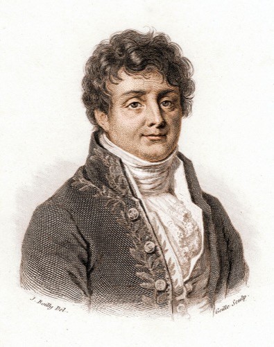 Joseph Fourier (1768–1830) reached his transform not through pure mathematics but through physics: the conduction of heat. In the 1822 Théorie analytique de la chaleur he made the then-scandalous claim that any function, however jagged, can be written as a sum of sines and cosines; contemporaries including Lagrange doubted it, and pinning down exactly when it holds occupied analysts for a century after. The decomposition into frequencies that diagonalizes convolution (the engine of this whole chapter) is his. (Fourier also argued that the atmosphere keeps the Earth warmer than incoming sunlight alone would: the first description of what we now call the greenhouse effect. He was, briefly, Napoleon's governor of Lower Egypt, too.) Portrait: engraving after Julien-Léopold Boilly, early 19th c., public domain (via Wikimedia Commons).
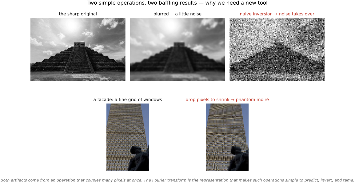
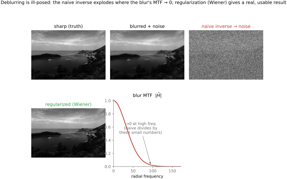
Fourier analysis rests on a change of representation: treat an image or signal as a sum of sine waves instead of a grid of pixels. It lets us answer rigorously the questions the previous chapters raised, and see what is possible, hard, or impossible. Start with two simple operations (Figure 6.3.1). First, deblurring: take a blurry photo for which we know the linear blur process but where noise further degrades the image. Try to undo the blur with direct linear inversion. Instead of the sharp original, the result explodes into noise. Second, downsampling: shrink a photo of a building facade by simply keeping every seventh pixel, and bold curved bands appear that are nowhere in the building: phantom moiré. Neither result is a bug; both are doing exactly what we asked. What makes them so hard to reason about is that each operation couples a great many pixels at once: a blur mixes every neighbor into every output, and decimation's fate depends on how the discarded pixels related to the kept ones across the whole image. Staring at the pixels tells us nothing. To understand how these artifacts and patterns emerge, and how to predict, invert, and tame them, we need a different mathematical tool, one in which these many-pixel operations become simple enough to analyze at a glance. That tool is the Fourier transform.
For the very same reason (that it captures blur so cleanly), Fourier is also the standard language for evaluating imaging systems. Because a lens or sensor blurs by convolving with its point-spread function, its contrast transfer can be described locally in the frequency domain by a modulation transfer function (MTF): how much contrast survives at each spatial frequency. MTF curves are how optics are actually specified and resolution is measured (a section below returns to this), so the machinery we build here to fight blur is the same machinery the industry uses to measure it. The eye works this way too: its own sensitivity to detail is a function of spatial frequency, the contrast sensitivity function (CSF) of Chapter 3.4, Spatial and temporal vision, so the frequency picture matches how we see as well as how lenses blur.
Fourier also describes wave propagation. In a suitable coherent optical setup, a lens maps the input field amplitude to its Fourier transform in a focal plane. A detector measures the squared magnitude of that field. This distinction matters when using Fourier to explain diffraction.

Fourier is useful even when we never compute a spectrum. It explains why blur is difficult to invert and why sampling creates aliases. It also supplies practical algorithms: FFT convolution, frequency-domain deconvolution, and transform coding. JPEG uses a related cosine transform (Chapter 8.11, File formats and compression).
A finite DFT represents a periodic signal. Padding lets an FFT compute ordinary finite convolution exactly; failing to pad instead computes circular convolution. We distinguish these boundary choices below.
Why Fourier⧉
optionalWe saw in Chapter 6.2, Convolution that convolution is a linear operator, and a linear operator is just a matrix. Stack an image's pixels into one long vector $\mathbf{x}$, and a blur becomes a single large matrix $M$ that carries the sharp image to the blurred one, $\mathbf{y} = M\mathbf{x}$. Here is the catch. That matrix is enormous, and painful to reason about and, above all, to invert: undoing the blur means untangling all the overlapping neighborhoods at once, and a clean, local operation can have a thoroughly non-local undo. You cannot eyeball a million-by-million matrix and pronounce whether it can be undone. For zero-extended one-dimensional convolution, the matrix is Toeplitz, the same kernel sliding down every row, constant along each diagonal, clean enough to draw. In 2-D that tidiness fragments: once you flatten the grid into a vector, the matrix becomes a block-of-Toeplitz-blocks, far messier to picture even though it is doing the very same local averaging. That is one more reason to change basis rather than wrestle the matrix directly.
There is, however, one species of matrix that is trivial to understand and trivial to invert: a diagonal matrix. A diagonal matrix has no cross-talk: each input coordinate is multiplied by its own scalar, independently of every other. Inverting it is then trivial: divide each coordinate by that scalar. The entire difficulty of inversion shrinks to one question per coordinate: how close is that scalar to zero? Dividing by a near-zero number is where all the trouble lives.
So the goal is clear: we would love the blur matrix to be diagonal. In the pixel representation it is nowhere close. But, and this is the pivot of the chapter, we are free to change how we represent the image, to describe it in a different basis, and a linear operator that looks coupled and hard to invert in one basis can look perfectly diagonal in another. The basis that diagonalizes convolution is precisely the Fourier transform. Change to the Fourier representation and blur stops being a million-dimensional tangle and becomes, instead, a separate scalar multiplication on each frequency, exactly the diagonal case we wished for. (For finite arrays, the DFT diagonalizes circular convolution. An ordinary finite convolution can be embedded in a larger circular one by padding, as the implementation below shows.)
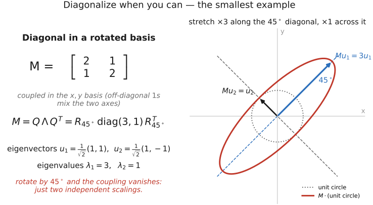
Express a linear operator in a basis where it becomes diagonal. A coupled, hard-to-invert operation in one representation can be a list of independent scalar multiplications in another, and scalars are trivial to understand, compose, and invert. Fourier diagonalizes convolution, turning a blur into per-frequency multiplication. This is not a one-off trick: it is the single most reusable move in applied linear algebra, and it returns for differential equations (the heat equation, below), for principal components, and for nearly every inverse problem in this book. The idea is already visible in the smallest possible case, a $2\times2$ matrix (Figure 6.3.3).
And there is a bonus that makes Fourier feel less like a computational convenience and more like the right language for images. We have already met spatial frequency once, back in perception: the contrast sensitivity function (CSF) describes the eye's sensitivity as a function of how fine or coarse a pattern is, its spatial frequency (see Chapter 3.4, Spatial and temporal vision). The visual system is, to a first approximation, organized by frequency. So the Fourier view matches both the mathematics of convolution and the structure of human vision, which is why frequency keeps reappearing: in JPEG compression, in image-quality metrics, in tone mapping. When two unrelated considerations point at the same representation, that representation is usually the one to learn.
Complex waves are eigenvectors of shifts and convolution⧉
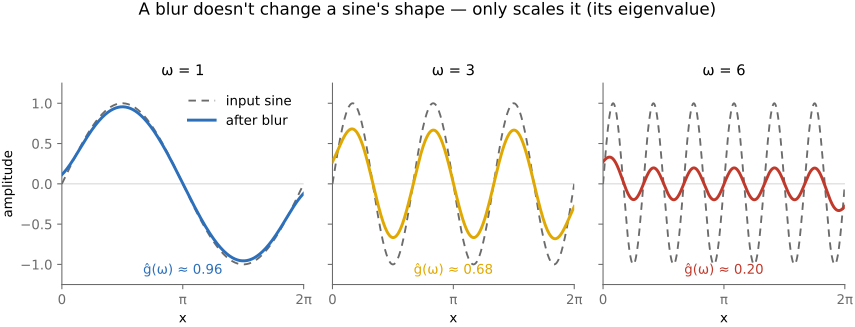
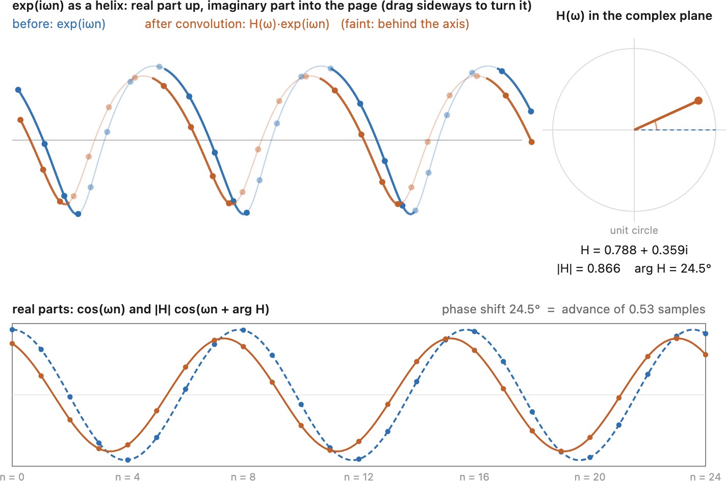
optionalWe have asserted that Fourier diagonalizes convolution. Here is the one-line reason, and it is the mechanical heart of the chapter. Start with the simplest operator of all, a plain shift. Slide a complex sine wave $e^{i\omega x}$ over by $d$ and you get $e^{i\omega(x - d)} = e^{-i\omega d}\,e^{i\omega x}$: the same wave at the same frequency, only multiplied by a constant phase $e^{-i\omega d}$. A complex exponential is therefore an eigenvector of translation, its frequency untouched and its eigenvalue a pure phase. Now recall that a convolution is nothing but a weighted sum of shifts (the sum-of-translated-images reading of the previous chapter). A weighted sum of shifts acting on our wave is a weighted sum of phases, still one number times the same wave, so a complex exponential is automatically an eigenvector of every convolution as well. Concretely, feed a pure sine wave into any convolution, any blur, and what comes out is the same sine wave, same frequency, only with its amplitude scaled and its phase possibly shifted (Figure 6.3.4). The wave is never bent into a different frequency; it is merely turned down (or up) and slid over. In the language of linear algebra, the complex exponentials are the eigenvectors of convolution, and the per-frequency scale factor is the eigenvalue. Symbolically, convolving a wave $e^{i\omega x}$ by a kernel $g$ just multiplies it by a number $\hat g(\omega)$ that depends only on the frequency:
A shift-invariant linear filter preserves frequency. Its complex gain can change amplitude and phase. A normalized smoothing kernel has gain one at DC and generally attenuates fine detail, but its response need not decrease monotonically: a box filter has zeros and side lobes. A real sinusoid stays sinusoidal; when its phase changes it is not, by itself, a real eigenvector.
Because every frequency is scaled independently, the whole convolution, written in the Fourier basis, is diagonal: the eigenvalues $\hat g(\omega)$ sit on the diagonal and nothing else. This is the convolution theorem, and it is the sentence to memorize:
Convolution in space is multiplication in frequency: transform the image and the kernel, multiply their spectra frequency by frequency, transform back. Everything else in this chapter is a consequence of that single identity.
Once you accept that a kernel's Fourier transform is its per-frequency gain, you can read a filter's entire behavior off the shape of $\hat g$, and conversely recognize a kernel from its spectrum. We gather the handful of kernels that recur most, and their spectra, alongside the other canonical transform pairs in the bestiary below.
The tiniest Fourier transform in the West⧉
optionalA million dimensions is impossible to picture, so shrink the image to two pixels, a vector in the ordinary 2-D plane, with the two pixel values as its $x$ and $y$ coordinates (Figure 6.3.6). Take the simplest blur: each output pixel is $0.8$ of itself plus $0.2$ of its neighbor. As a matrix in the pixel basis this mixes the two coordinates: it is not diagonal; the off-diagonal $0.2$ is the cross-talk.
Now rotate the coordinate axes by 45°, onto the two directions $[1, 1]$ (both pixels equal, the constant, the zero-frequency or direct current (DC) term, borrowing the electrical-engineering name) and $[1, -1]$ (the two pixels opposite, the highest frequency a two-pixel image can carry). These two orthogonal axes give the normalized two-point Fourier transform. The displayed matrix includes a reflection, so it is an orthogonal change of coordinates rather than a pure rotation. And in these rotated axes the very same blur is diagonal: the constant direction $[1, 1]$ passes through untouched (a flat signal cannot be blurred, eigenvalue $1$), while the oscillating direction $[1, -1]$ is attenuated to $0.6$ (since $0.8 - 0.2 = 0.6$, the high frequency is damped). Two pixels, two frequencies, two independent scale factors: the entire apparatus of the chapter in a picture you could draw on a napkin. Everything that follows is this, scaled up to a million dimensions.
Written out, the change of basis and the blur it diagonalizes are just $2\times2$ numbers: the two-point DCT $B_2$ conjugates the blur $M$ into a diagonal of its eigenvalues.
The two rows of $B_2$ are the DC and the highest-frequency wave; conjugating by them turns the off-diagonal mixing into two independent gains, $1$ and $0.6$.
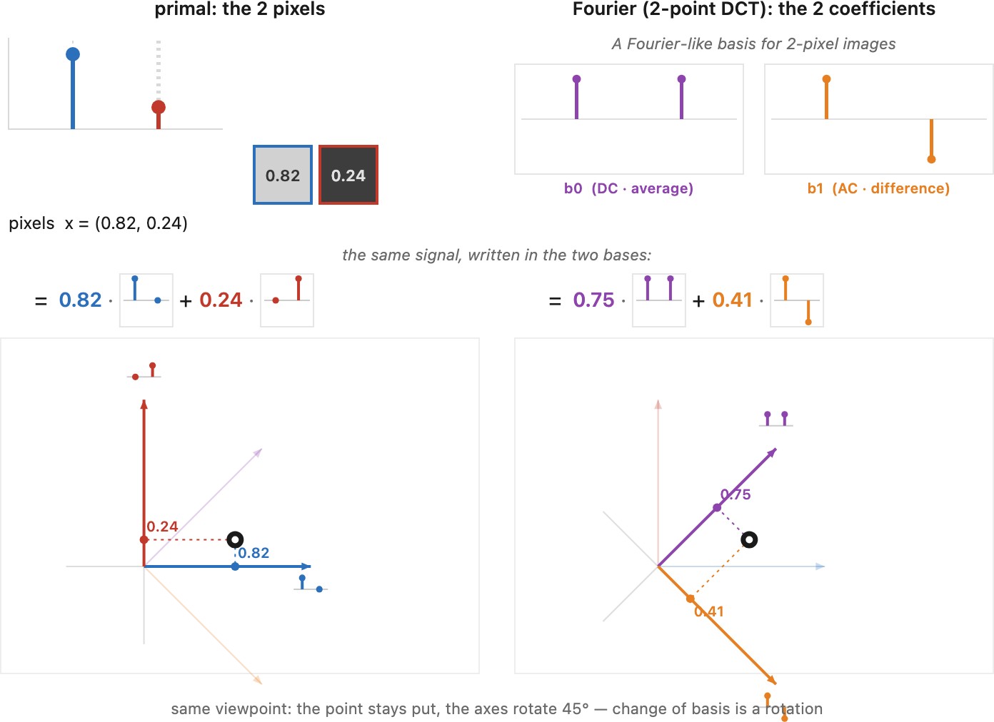
There are two ways to picture a change of basis, and they are worth holding apart: either the point stays fixed in space and the axes rotate around it, or you redraw both frames the same way and the point's coordinates move, transformed by the change-of-basis matrix. Same fact, two views; the 2-pixel figure above lets you toggle between them.
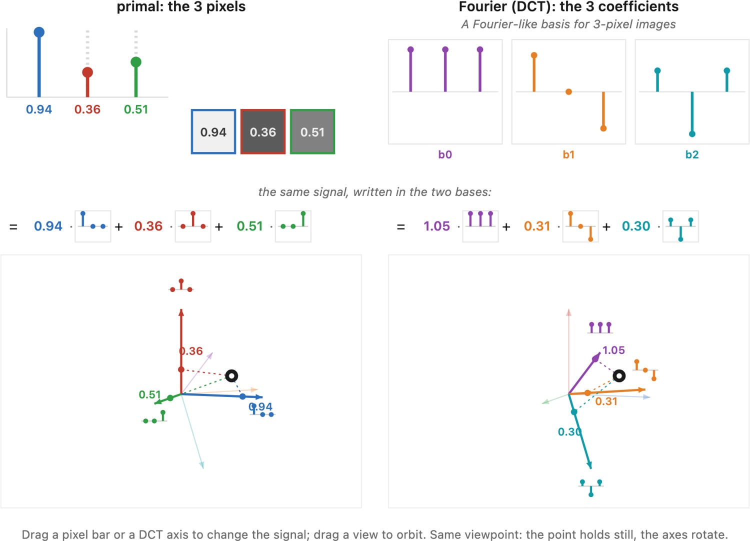
A three-pixel image is a point in 3-D. To keep this illustration real, we use the discrete cosine transform (DCT), whose axes here are a constant, a ramp, and a cosine (Figure 6.3.7). The DCT is related to Fourier analysis through an even extension of the signal. It is a different transform from the three-point DFT, whose nonconstant coefficients are complex.
Its matrix is again just numbers, the orthonormal three-point DCT, whose rows are the flat, ramp, and single-cosine waves.
The rows are orthonormal: lengths and angles are preserved, and the transpose gives the inverse. This matrix has determinant $-1$, so it includes a reflection.
Definition: one coefficient per wave⧉
optionalHere is the transform itself, in words first. Instead of describing an image by one value per pixel, the Fourier transform describes it by one coefficient per sine wave. We fix a family of sinusoidal patterns, waves of every frequency that fit in the image, and ask, for each one, how much of that wave is present? The list of answers is the Fourier transform $\hat I$ of the image, and because the operation is perfectly reversible, that list carries exactly the same information as the original pixels: it is the same image, written in a different alphabet.
For an $N$-sample one-dimensional signal the recipe is a sum: one output coefficient $\hat I(u)$ for each frequency index $u$. This is the discrete Fourier transform (DFT):
Read it back in words: to find how much of frequency $u$ the signal holds, slide a wave of that frequency across the signal, multiply point by point, and add up, a dot product between the signal and that wave. The complex exponential $e^{-2\pi i\,ux/N}$ is just a compact way to carry a cosine and a sine of frequency $u$ together, by Euler's formula
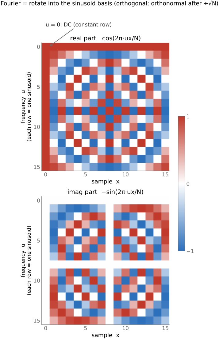
so the real part of $\hat I(u)$ measures the cosine content and the imaginary part the negative of the sine projection. Why carry both? Because a single frequency can appear at any phase, shifted left or right, and a cosine and a sine of that frequency together can reproduce a wave of that frequency at any phase and amplitude. One pair, one cosine and one sine, per frequency. (The naive sum costs $O(N^2)$, but the fast Fourier transform (FFT) computes the very same coefficients in $O(N\log N)$, the algorithm that made Fourier methods practical, and the reason spectral tricks are cheap in code.)
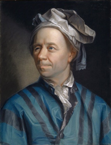 Leonhard Euler (1707–1783) was the most prolific mathematician who ever lived: he kept publishing for years after going blind, dictating from memory. The formula just above, $e^{i\theta}=\cos\theta+i\sin\theta$, is his, and it is what lets a single complex exponential carry a cosine and a sine together, the bookkeeping that makes the Fourier transform compact. His reach into this book is wide: the Euler–Lagrange equations we set to zero to minimize an energy (optical flow, Poisson blending), and the Eulerian "watch a fixed location" view of motion that names half of Chapter 12.4, Feature tracking and all of Chapter 38.3, Motion and video magnification. Portrait: by Jakob Emanuel Handmann, 1753, public domain (via Wikimedia Commons).
We use a negative exponent on the forward DFT and divide the inverse by the number of samples. Check the sign, normalization, and frequency units when translating formulas into code. A continuous transform, a Fourier series, and a finite DFT also describe different signal domains; they are not interchangeable definitions of the same array operation.

The waves are mutually orthogonal. With our unnormalized forward transform, each row of its matrix $F$ has norm $\sqrt N$, so $F^{-1}=F^*/N$, where $F^*$ is the conjugate transpose. Dividing both transform matrices by $\sqrt N$ gives the unitary convention used in geometric illustrations. The inverse of our DFT is
It adds the waves with their complex coefficients. The frequency index $u$ corresponds to $u/N$ cycles per sample, with indices above half the array interpreted as negative frequencies. In two dimensions the exponent becomes $-2\pi i(ux/W+vy/H)$, we sum over both pixel coordinates, and the inverse has factor $1/(WH)$.
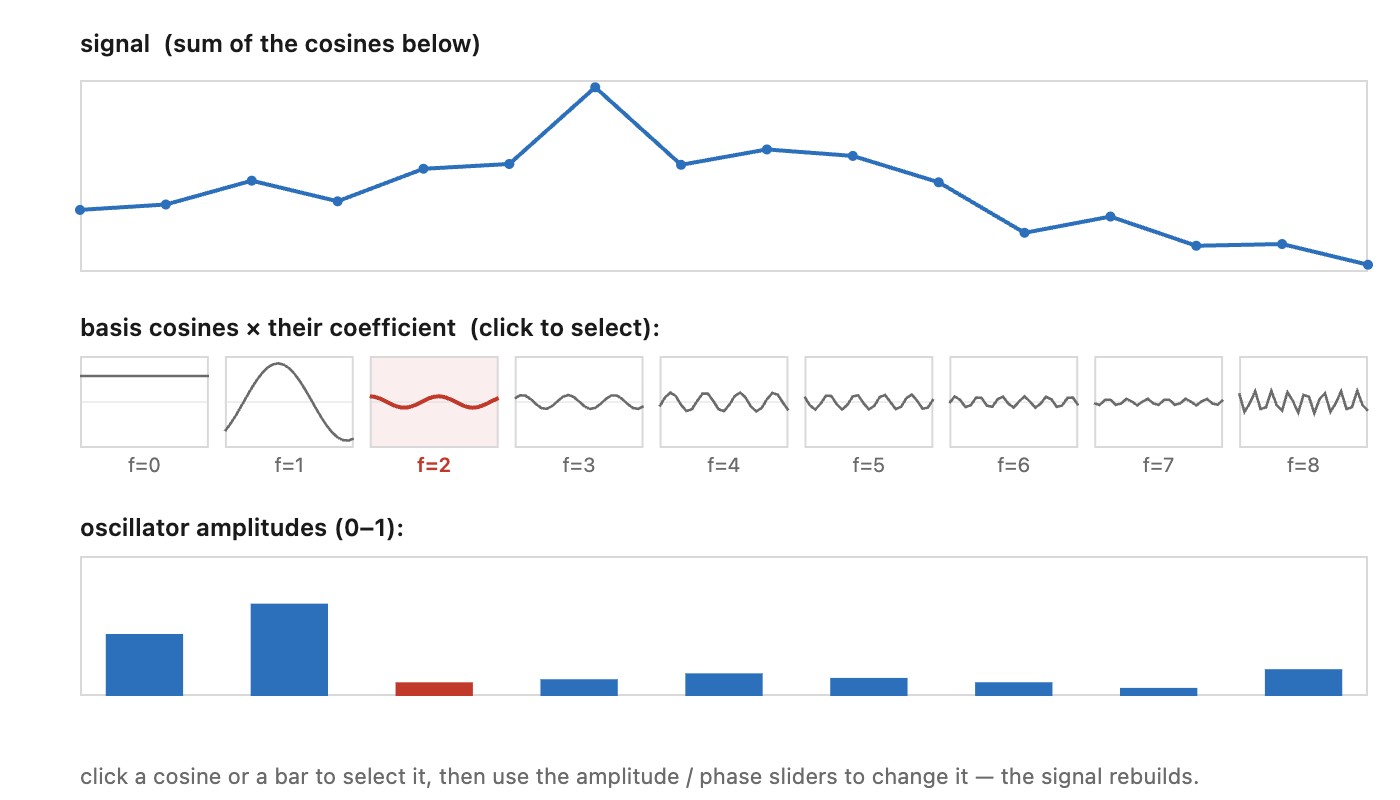
Read that inverse the other way and it becomes the most concrete statement of what the transform means: the signal is the sum of the basis waves, each weighted by its own coefficient. It is easiest to feel in one dimension first (Figure 6.3.10): a short signal is a sum of cosines, one per frequency, and adjusting a single wave's amplitude and phase reshapes the signal in the obvious way.
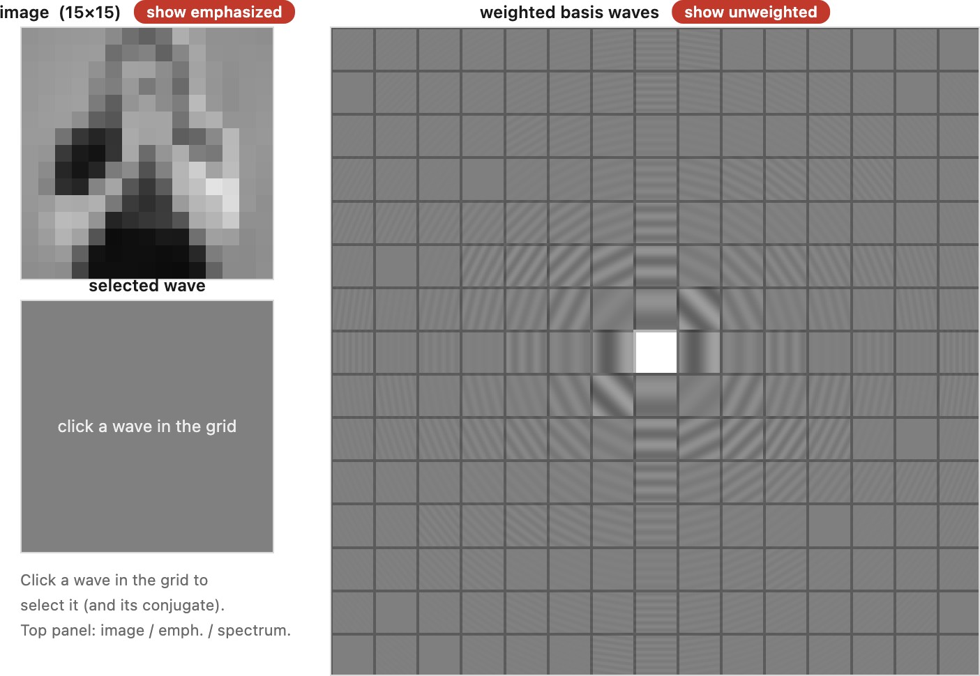
The same holds for an image, now with waves in two dimensions. Every picture, however busy, is a stack of plain 2-D sinusoids added together, and the Fourier transform is nothing more than the list of how much of each one to add. You can see this directly (Figure 6.3.11): dial the resolution down to a handful of waves, watch a recognizable image fall out of their sum, and click any single wave to see exactly what it contributes.
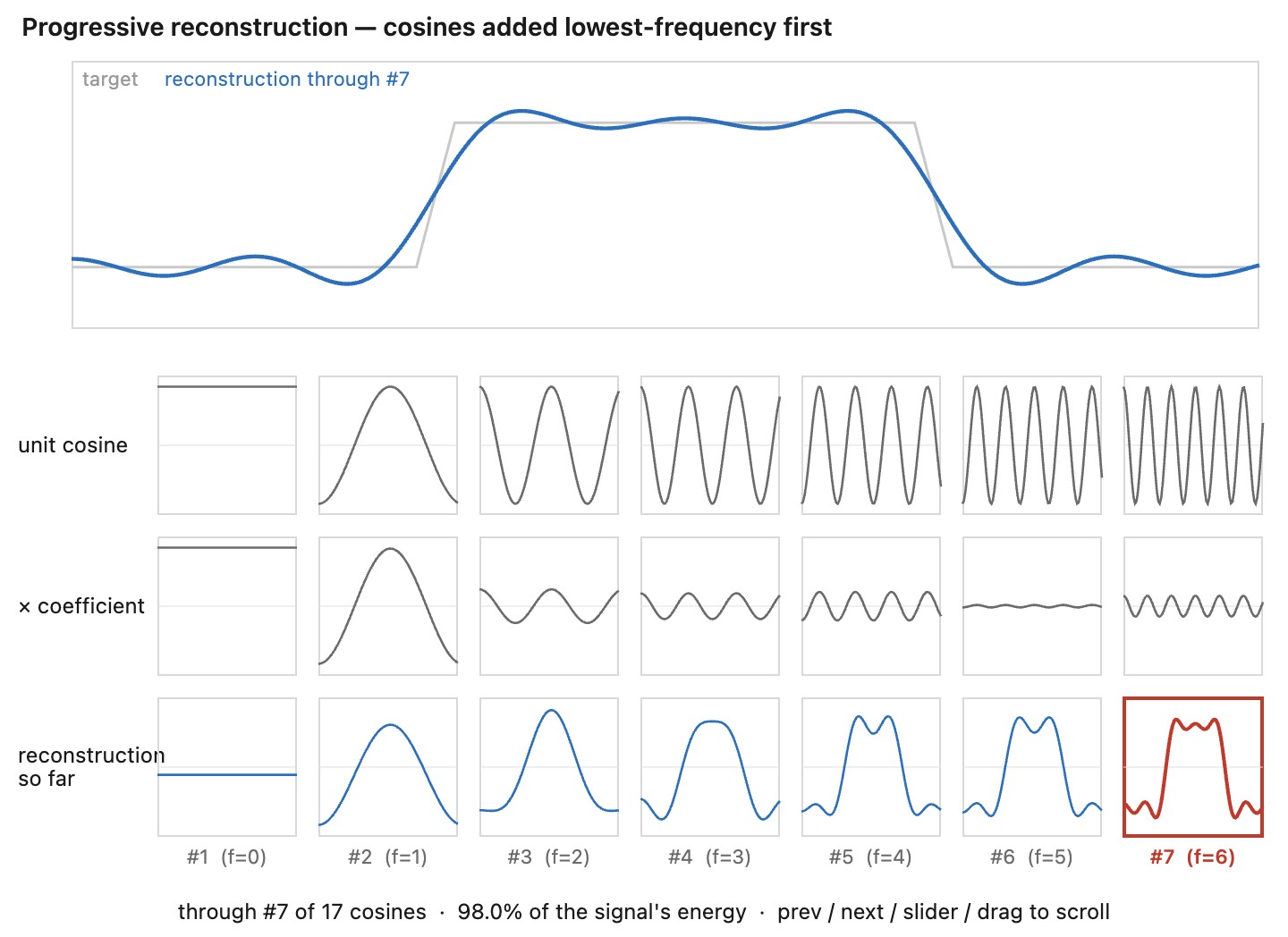
We can add waves in increasing frequency order, or in decreasing contribution to signal energy (Figure 6.3.12). A low-pass reconstruction of a sharp pulse rings near its edges. For a continuous discontinuity, Fourier-series overshoot persists while its affected region narrows, the Gibbs phenomenon. A finite DFT with every coefficient restored reproduces the original samples exactly; the intermediate ringing must disappear at those samples.
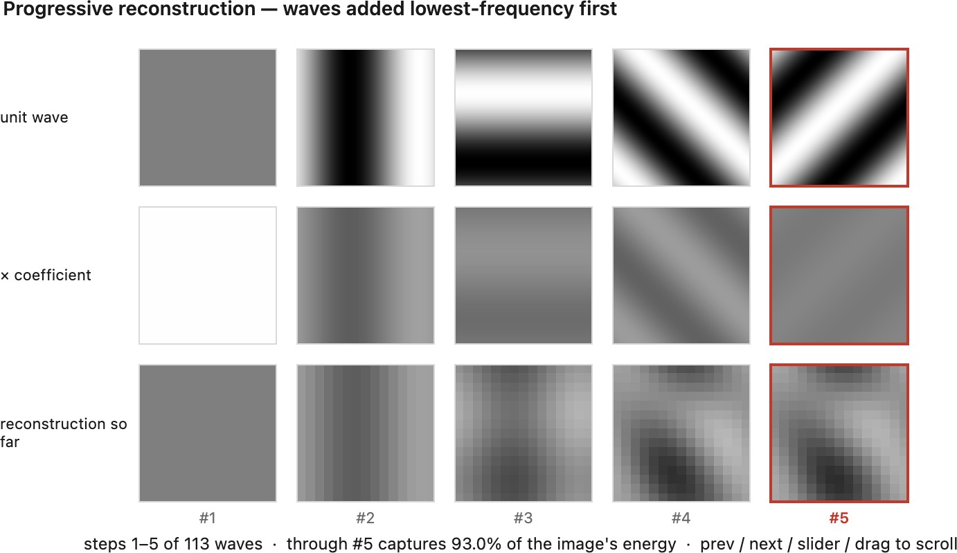
The same two orderings carry over to an image (Figure 6.3.13). Add the waves back lowest-frequency first and the picture blurs in from coarse to fine, the smooth tone first and the sharp detail last; sort them instead by amplitude, largest first, and it assembles from the highest-energy strokes down. Either way the striking part is how few waves it takes: a handful already give a recognizable image, because a natural photograph packs most of its energy into a small number of low frequencies. That concentration is exactly what image compression exploits, keeping the large coefficients and discarding the swarm of tiny ones, and it is the thread we pick up again with the DCT and JPEG.
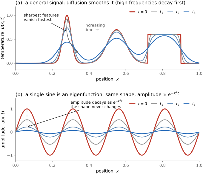
This Fourier transform was not invented for images. Jean-Baptiste Joseph Fourier (1768–1830) was trying to solve heat diffusion in a one-dimensional rod with a given initial temperature profile, and the governing equation was a coupled mess. His move, in 1807, was to write the temperature as a sum of cosines, and in that basis the heat equation diagonalizes: each frequency evolves entirely on its own, and a single cosine simply decays exponentially in time ($\propto e^{-k^2 t}$), the highest frequencies fastest, so any profile smooths out. The cosines are the eigenfunctions of the Laplacian (the diffusion operator), the same reason Fourier diagonalizes our convolutions. Notice what separation of variables has handed us: the two canonical solution families of linear differential equations meeting in one problem, sine waves in space and exponentials in time. The spatial sinusoids set the basis; their amplitudes decay as $e^{-k^2 t}$, the finest ripples dying first, so a general profile melts smooth while a single sine merely fades in place without changing shape (Figure 6.3.14). The lesson reaches far past heat: for almost any linear ordinary differential equation (ODE) or partial differential equation (PDE), find the eigenbasis and a coupled system decouples into independent scalar equations whose solutions are plain exponentials ($e^{\lambda t}$) or, for oscillatory systems, sine waves. Diagonalizing is the win.
Everything above assumed a grayscale image, one coefficient per wave. Color needs nothing new: run the same transform on each channel, giving three sets of coefficients. Every statement here holds channel by channel, so we develop it in grayscale and apply it thrice.
The matrix view makes the computation especially concrete. Put one sampled basis wave in each row of the transform matrix, using the complex conjugate for the forward projection. Multiplying that row by the image computes one coefficient. There is no separate linear system to solve because the basis waves are orthogonal; normalization supplies the inverse scale. The same basis works for every circular convolution, so changing the blur changes the diagonal gains rather than the basis itself.
Reading an image's Fourier transform⧉
optionalFor a 2-D image the recipe is the same with two frequency indices $(u, v)$, horizontal and vertical, so the transform is itself an image, the same size as the original, with a value at each frequency. We display it as two pictures: a magnitude (how much of each frequency is present) and a phase (where each wave sits). A handful of properties make these readable.
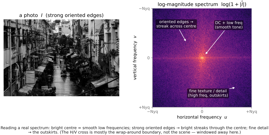
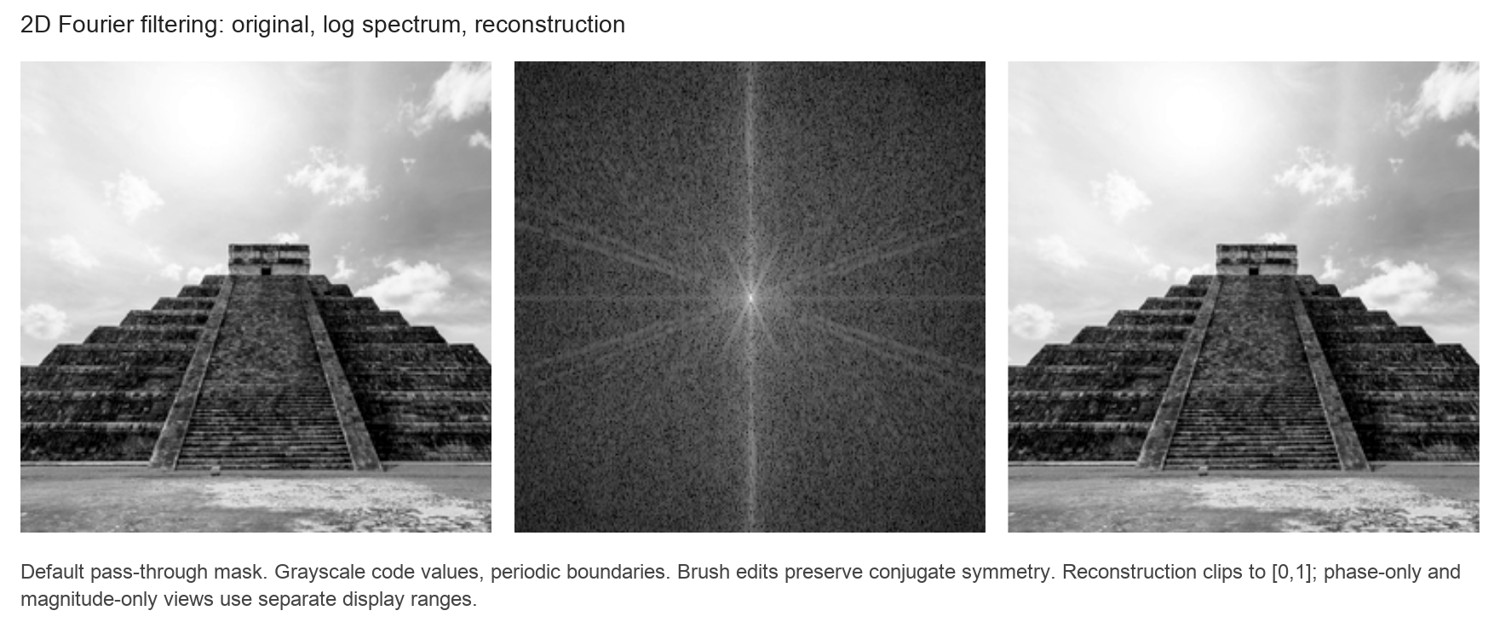
First, a real image has a conjugate-symmetric spectrum: the coefficient at frequency $(u, v)$ is the mirror of the one at $(-u, -v)$, so half the coefficients are redundant and the magnitude image is point-symmetric about its center. The very low frequencies (slow, large-scale variation) sit near the center; the high frequencies (fine detail, sharp edges) sit out toward the corners. Many photographs have larger individual coefficients at low frequencies, so a typical per-coefficient magnitude spectrum is bright in the middle and dim at the edges, often with bright streaks where strong oriented structure (a horizon, a picket fence) lives. Set a real photograph beside its log-magnitude spectrum and you can read these correspondences off directly (Figure 6.3.15): the bright center is the smooth tone, oriented scene edges show up as bright streaks through the center, and fine texture fills the outskirts. (Beware: the cyclic wrap-around assumption itself injects a cross of horizontal and vertical power, from the discontinuity where the image's left edge meets its right; serious analysis windows the image first to suppress it.)
A second reading aid is to manipulate the spectrum and watch what returns. Because filtering is multiplication in frequency, we can low-pass or high-pass a real photo by hand: transform it, multiply the spectrum by a mask, a disk that keeps only the center, or its complement that keeps only the outside, and transform back (Figure 6.3.17). Keep the center and the fine detail is gone: a smooth, blurred image, since the detail lived in the high frequencies we deleted. Keep the outside and only the edges and texture survive, the smooth tone subtracted away. This is the convolution theorem turned into an operation you can watch.
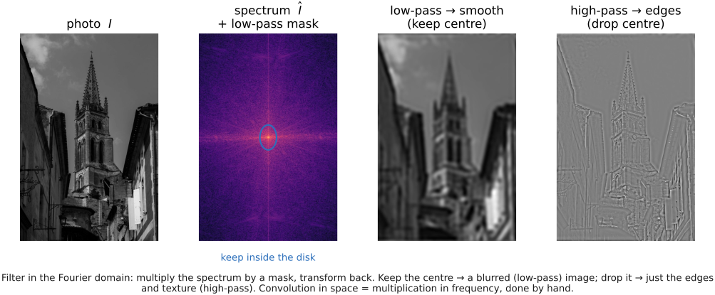
This low-pass/high-pass split is so useful that retouchers reinvented it by hand, without ever transforming to the frequency domain. The technique is called frequency separation, and it is a staple of portrait and product editing in Photoshop: blur a duplicate layer to isolate the low frequencies (the smooth tone and color transitions), subtract that from the original to recover the high frequencies (the pores, hairs, and fine texture) on a second layer, and then edit each independently: even out blotchy skin tone or color on the low-frequency layer while leaving pore detail perfectly crisp on the high-frequency layer, or vice versa. It is exactly the two-band decomposition above (a low-pass plus its high-pass complement, which sum back to the original), arrived at pragmatically by photographers who needed to touch tone and texture separately; the major retouching tutorials walk through the layer recipe in detail (Frequency separation (Photoshop retouching technique)).
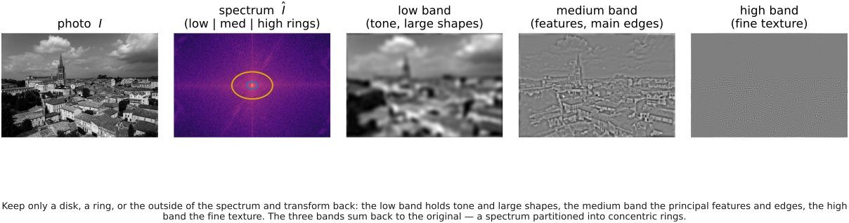
Splitting the Fourier coefficients into three disjoint regions gives low, medium, and high frequency components (Figure 6.3.19). Their sum reconstructs the image exactly because each coefficient belongs to one region. The visual importance and energy of a band depend on the image and cutoffs. Laplacian pyramids offer a related multiscale representation with overlapping responses rather than sharp frequency partitions (Chapter 6.6, Pyramids and wavelets).
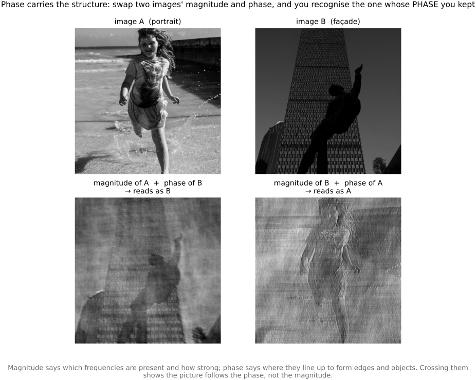
Phase describes how waves line up to form edges and objects. Swapping the phases of two photographs often makes each reconstruction resemble its phase donor (Figure 6.3.21). Magnitude still matters: it determines contrast and the strength of each frequency, and can contain substantial information about shape and texture. A coefficient of zero magnitude has no defined phase.
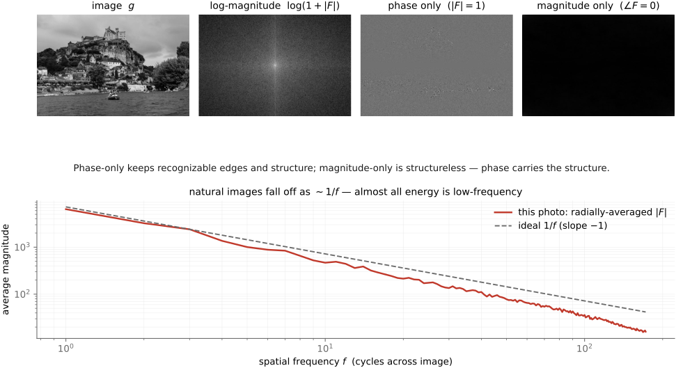
Try the swap on two photographs with broadly similar magnitude spectra. Their common spectral statistics make the importance of phase especially visible. It is a useful demonstration, not a guarantee for arbitrary images: replacing the magnitude by zeros, or retaining only a few frequencies, destroys the picture regardless of its phase.
Phase specifies the alignment of the waves; magnitude specifies their strength. Phase swaps between typical photographs often preserve recognizable structure from the phase donor, but accurate reconstruction requires both.
A circular shift of a finite image changes only phase: shifting by $(d_x,d_y)$ multiplies each coefficient by $e^{-2\pi i(ud_x/W+vd_y/H)}$, whose magnitude is one. A translation of an unbounded signal obeys the same rule. Translating and cropping a photograph also changes its contents, so its magnitude spectrum need not stay fixed. General convolutions can change magnitude as well as phase.
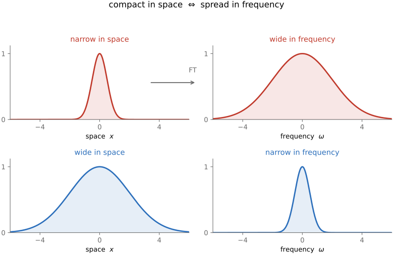
Fourth, the compact-in-space / spread-in-frequency tradeoff. A narrow, sharply localized blob in the image has a wide spectrum, and a wide smooth blob has a narrow one (Figure 6.3.22). A Gaussian makes this exact: the narrower the Gaussian in space, the wider its Fourier transform, which is itself a Gaussian. You cannot be compact in both domains at once. This locality-versus-frequency tradeoff is a genuine uncertainty principle, and it is the reason we will later want pyramids and wavelets, which sit halfway between the pixel and Fourier representations to buy some localization in both.
View each inverse-transformed band on its own before adding them. The low band gives a blurred arrangement of large light and dark regions. The high band often looks like faint signed texture on a gray background because a display offset is needed to see negative values. A faint-looking band can still matter at an edge, so compare both its energy and the visual effect of omitting it. Returning the three disjoint coefficient sets to the spectrum reconstructs the original; clipping the displayed band images before summing would not. This separates the decomposition from its visualization (Figure 6.3.19).
A small bestiary of transforms⧉
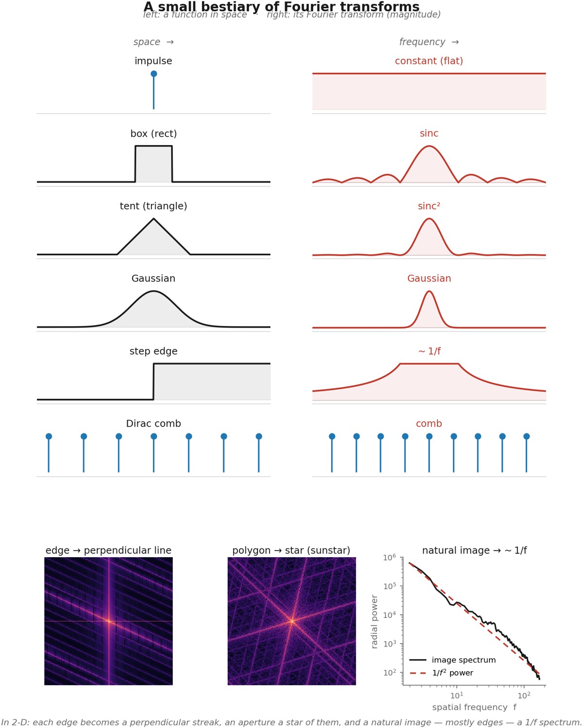
optionalA handful of shapes recur so often that knowing their transforms by sight is most of the working intuition. Each pairing reinforces the space–frequency tradeoff (narrow here = wide there) and connects back to operations we already use (Figure 6.3.23).
- Impulse (delta) ↔ constant. A single bright point contains every frequency in equal measure, a flat spectrum; conversely a constant (DC) is a single spike at zero frequency. This is why a point source probes a system's whole frequency response: the PSF's transform is the optical transfer function (OTF); its normalized magnitude is the MTF.
- Box (rect) ↔ sinc. A unit-area continuous box of width $w$ transforms to $\operatorname{sinc}(w f)$, a central lobe with side-lobes that decay only as $1/f$. Wider box → narrower sinc. A hard frequency cutoff therefore produces a ringing spatial kernel. A spatial box average has nonnegative weights and cannot overshoot a step.
- Tent (triangle) ↔ sinc². A triangle is a box convolved with itself, so its transform is the box's squared, $\operatorname{sinc}^2$, whose side-lobes now fall as $1/f^2$, giving stronger high-frequency attenuation. Both spatial box and tent averages have nonnegative weights and cannot overshoot a step.
- Gaussian ↔ Gaussian. The Gaussian is (up to scale) its own transform: a smooth positive shape in both domains, and a narrow Gaussian ↔ a wide one, the space–frequency tradeoff in its purest form.
- Step edge ↔ ~$1/f$. A sharp step's spectrum falls off as $1/f$ (its derivative is an impulse, flat in frequency; integrating divides by $f$). The full transform also includes a DC term; the $1/f$ statement describes its nonzero-frequency component.
- Comb ↔ comb. A train of impulses transforms to another train of impulses, the fact behind sampling, in the next chapter.
An infinite straight edge varies only perpendicular to itself, so its transform is supported on the corresponding frequency line. Finite edges broaden this support. Aperture edges similarly help explain the directions of diffraction spikes, but the observed intensity is the squared magnitude of the transform of the entire aperture. Many natural photographs have an approximately $1/f$ average amplitude spectrum, or $1/f^2$ power spectrum, over a limited range. This is an empirical statistical regularity. In two dimensions, larger annuli contain more coefficients: a $1/f^2$ power spectrum gives roughly equal non-DC energy per octave, not almost all energy in the lowest octave.
Natural photographs often have approximately $1/f$ average Fourier amplitude over a range of scales. Distinguish amplitude from power, and average power per coefficient from total energy in a frequency band. The image mean can dominate total energy without explaining its visible detail.
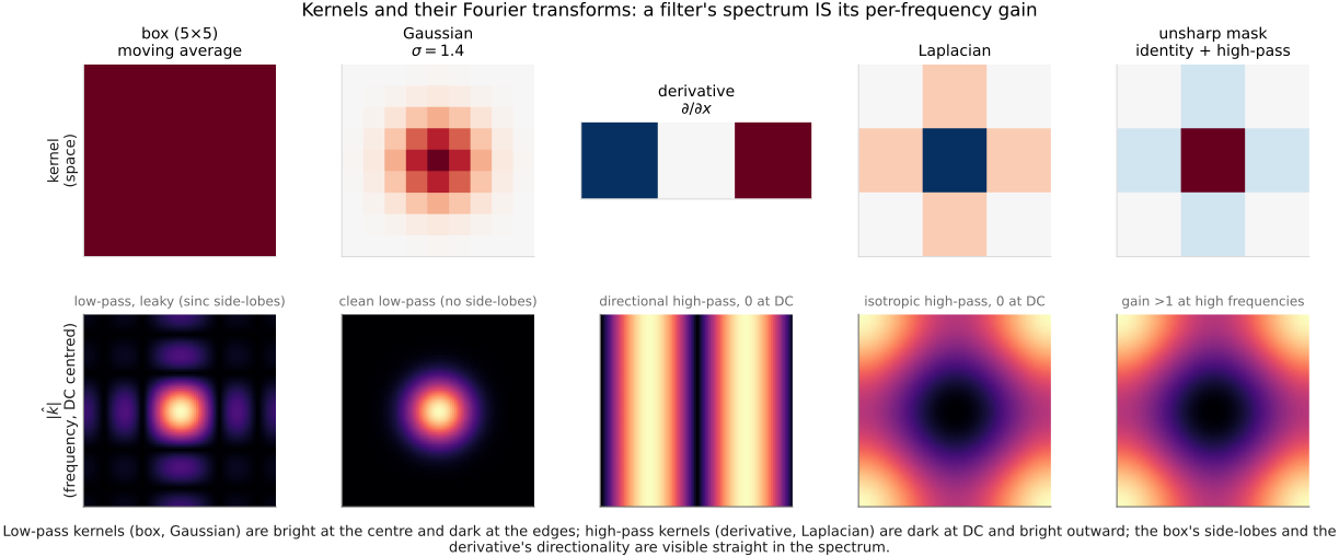
The frequency response also distinguishes practical kernels (Figure 6.3.24). A sampled box has zeros and side lobes, so it suppresses some high frequencies much less than others. A continuous Gaussian has a Gaussian transform; sampling and truncating it perturb that ideal. Derivatives kill DC, but their discrete responses depend on the stencil: a centered difference also vanishes at Nyquist. A Laplacian suppresses constant regions, while unsharp masking raises the gain of selected detail frequencies above one. Use the transform of the actual discrete kernel when predicting an implementation.
Application preview: can we deblur, given the blur?⧉
optionalWe can finally settle the promise. Suppose we know the blur, the kernel $g$ the optics applied, and we are handed the blurred image; this is non-blind deconvolution (the harder blind case, where the kernel is unknown, waits for a later chapter). The Fourier view makes the question crisp. In the frequency domain, blurring multiplied each frequency of the sharp image by the kernel's eigenvalue: $\hat I_\text{blur} = \hat I_\text{sharp} \cdot \hat g$. To invert, just divide it back out:
This is inverse filtering. It is exact for noiseless data wherever the response is nonzero. A blur diagonalized into per-frequency multiplications is undone by per-frequency divisions. So why is deblurring not a solved problem?
Because of the one number we said decides everything: how close the eigenvalue is to zero. A blur is a low-pass filter, so $\hat g$ is large at low frequencies but tiny, near zero, at exactly the high frequencies the blur destroyed. Dividing by a near-zero number is catastrophic. And real images carry noise: a little random grain the sensor added after the blur, so that what we actually observe is $\hat I_\text{blur} = \hat I_\text{sharp}\cdot\hat g + \hat n$. Divide that through and we get $\hat I_\text{sharp} + \hat n / \hat g$: the genuine signal comes back, but the noise term is divided by $\hat g$ as well. At a high frequency where $\hat g \approx 0.01$ the blur attenuated the signal a hundredfold, yet it never touched the noise, which was added afterward, so dividing by $0.01$ now amplifies that noise a hundredfold. The inverse filter faithfully reconstructs the signal and, in the same stroke, explodes the noise; the result is a sharp-looking image drowned in colorful high-frequency garbage (Figure 6.3.28). This is the central difficulty of deblurring, and the Fourier picture diagnoses it exactly: inverse filtering is unstable precisely where the blur was strong.
A Wiener filter balances inversion against noise amplification. For independent, zero-mean stationary signal and additive noise with power spectra $S_I$ and $S_n$, the minimum-mean-square-error linear estimate uses
The star denotes complex conjugation. Where the signal dominates, the factor approaches $1/\hat g$; where noise dominates, it suppresses the measurement. Frequencies with no measured information cannot be recovered by division. This formula depends on the assumed spectra and boundary model; it does not claim to be the best nonlinear estimator. Chapter 7.1, Imaging as Bayesian inference with probabilistic priors develops the statistical interpretation.
In the Fourier basis a convolution is diagonal: it multiplies each frequency by one number (the kernel's complex response, the OTF), so undoing it is a per-frequency division. The whole stability question becomes local to each frequency: how near zero is that number? Blur is low-pass, so its response is tiny at exactly the high frequencies it destroyed; the lower a frequency's coefficient, the more its noise is amplified on inversion. That is why naive deblurring fails worst precisely where the blur was strongest, and why a Wiener / regularized filter stops dividing once the signal drops below the noise floor.
Convolution by FFT⧉
optionalThe fast Fourier transform (FFT) computes an $N$-sample DFT in $O(N\log N)$ operations. It changes the cost of the transform, not its definition. This makes spectral multiplication a useful way to compute large convolutions.
Direct convolution costs $O(NK)$ for $N$ output pixels and a kernel with $K$ taps. FFT convolution costs $O(P\log P)$ for a padded array with $P$ elements. The required padding grows with the kernel, so the cost is not completely independent of kernel size. Small kernels usually favor direct convolution; separable kernels have a cheaper direct implementation.
For zero-extended input of size $H\times W$ and a kernel of size $K_h\times K_w$, use transform dimensions at least $H+K_h-1$ and $W+K_w-1$. Here is full convolution with both arrays stored from index zero:
P = efficient_fft_size(H + Kh - 1, W + Kw - 1)
A = zeros(P); A[0:H, 0:W] = image
B = zeros(P); B[0:Kh, 0:Kw] = kernel
full = real(ifft2(fft2(A) * fft2(B)))
full = full[0:H+Kh-1, 0:W+Kw-1]
# For a centered odd kernel, crop from (Kh//2, Kw//2)
same = full[Kh//2:Kh//2+H, Kw//2:Kw//2+W]
The inverse includes its usual normalization. No fftshift is needed in this convention. For reflected boundaries, extend the image first and adjust the crop. Check an impulse and an asymmetric kernel to catch shifts and accidental correlation.
Running sums compute box filters in linear time. Repeated boxes and recursive filters approximate a Gaussian efficiently, while a separable finite Gaussian can be computed exactly in two passes. Compare approximation error as well as runtime. An arbitrary large PSF is a stronger case for FFT convolution (Chapter 29.1, Algorithmic speedups).
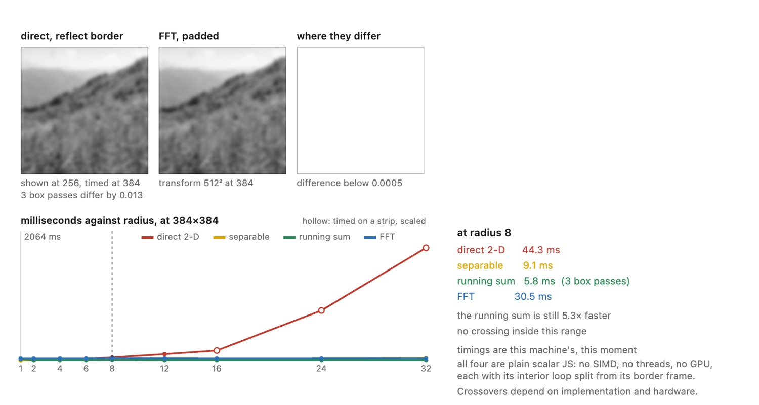
The FFT method pays for transforming a padded image, transforming a padded kernel, multiplying their coefficients, and transforming the result back. A small direct kernel performs only a few multiplies per pixel and avoids those transforms, so asymptotic complexity alone does not choose the faster method. A large nonseparable point-spread function can reverse that comparison. If many images use the same kernel, its transform can be reused. If the kernel is separable, compare against two one-dimensional direct passes rather than the more expensive two-dimensional baseline. Padding, boundary handling, and reusable transforms belong in the performance comparison as well as in the correctness check.
The radix-two Cooley–Tukey construction splits an even-length transform into transforms of the even-indexed and odd-indexed samples. Each half is reused when forming two groups of outputs, with known complex phase factors accounting for the odd positions. Recursing on the halves gives a logarithmic number of stages with linear work per stage. This is why the FFT computes the same coefficients as the direct sum with far fewer operations; it is not an approximate transform. Other factorizations handle other lengths.
Image formation as a linear system⧉
How solvable is an imaging problem?⧉
optionalThose two examples, a defocused lens you can barely invert and a corner camera you invert in one line, are a preview of the question this section addresses: given $A$ and a measurement $\mathbf{y}=A\mathbf{x}+\mathbf{n}$, how hard is it to recover $\mathbf{x}$?
Recovery depends on which variations the operator measures, their signal-to-noise ratios, and how accurately the operator is known. A null space leaves ambiguity; small gains make inversion sensitive to noise. An unknown or miscalibrated operator adds a separate estimation problem.
Before trying to invert anything, inspect $A$ to predict how the inverse will behave. Two properties tell you almost everything: the operator's shape and its conditioning (Figure 6.7.4).
A square, full-rank matrix determines one exact solution, though it can be sensitive to noise. A tall matrix has more measurements than unknowns, but only full column rank guarantees a unique least-squares solution. Repeated independent measurements can reduce noise; duplicate geometry does not fill an existing null space. A wide matrix necessarily has a null space. If $A\mathbf z=0$, then $\mathbf x$ and $\mathbf x+\mathbf z$ give the same noiseless data. Demosaicking illustrates this: one measured channel per pixel does not determine three unrestricted color values without additional assumptions.
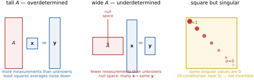
Before the general case, look at the easy one, because it organizes everything that follows: $A$ square and diagonal. Then the equation decouples completely (each measurement is just one unknown times one diagonal entry, $y_i = a_{ii}\,x_i + n_i$) and inverting is nothing but per-element division, $x_i = y_i / a_{ii}$. You can read the trouble straight off the diagonal: wherever an entry $a_{ii}$ is large the inversion is gentle, and wherever it is near zero the division blows the noise up. No subspaces, no entanglement, just a list of independent gains. This case matters because many operators can be made diagonal by a change of basis. For the convolutions that dominate imaging (blur, defocus, motion) the Fourier basis does exactly this (each frequency is rescaled on its own; → Chapter 6.3, Fourier), turning deblurring into per-frequency division and ill-conditioning into simply the frequencies the blur zeroed out. Diagonalizable operators are the ones we truly understand.
Now conditioning, which is subtler and where most of the real pain lives, because even a square, technically invertible $A$ can be useless. The plain way to see a general operator (one no single change of basis diagonalizes) is through its singular values: the set of gains $\sigma$ by which it stretches or shrinks the different directions of the scene, the diagonal case's "gains" generalized to any matrix. Inverting $A$ means multiplying each direction by $1/\sigma$. If the singular values run from large down to nearly zero (a large condition number $\kappa(A)=\sigma_{\max}/\sigma_{\min}$) then the directions with tiny $\sigma$ get multiplied by an enormous $1/\sigma$, and any noise that happened to land on those directions is amplified without mercy. A lens blur is the textbook villain: it attenuates high spatial frequencies almost to nothing (tiny singular values up there), so naive deblurring divides the noisy high frequencies by almost zero and the image dissolves into a blizzard. Figure 6.7.4 shows this in one dimension, and it is the picture to keep: the true signal, blurred and lightly noised; the operator's singular values decreasing toward zero; the naive inverse exploding into garbage; and a regularized inverse recovering the signal cleanly.
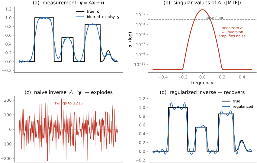
Singular values alone do not specify recoverability. Their scale depends on the units of the scene and measurement, and the noise level must be compared with the attenuated signal in each measured direction. Whitening accounts for unequal or correlated measurement noise before assessing the relative gains.
Hadamard calls a problem well-posed when a solution exists, is unique, and depends continuously on the data Hadamard 1902. A finite full-rank system can satisfy all three and still be badly conditioned: continuity does not guarantee small error amplification. Rank deficiency creates nonuniqueness, and noisy overdetermined equations can be inconsistent. These are distinct reasons to replace exact inversion with a statistical estimate.
A useful way to read the operator is to ask what happens to differences between candidate scenes. If two scenes produce exactly the same measurement, their difference lies in the null space; no noiseless inversion can tell them apart. If the measurements differ only slightly, noise may hide the difference even though the operator is technically invertible. Adding more equations helps only when they constrain directions that the earlier measurements left ambiguous. Repeating the same exposure can reduce independent noise, but it does not by itself add a missing spatial frequency or a new view.
When linearity breaks down⧉
optionalA caveat: the clean equation $\mathbf{y}=A\mathbf{x}$ is an idealization with real edges. Five departures matter.
First, clipping (see Chapter 2.8, Noise, signal-to-noise ratio and dynamic range). A photosite well holds only so many electrons and an encoded pixel only so many code values, so the moment a measurement saturates (a blown highlight, a crushed black) the response stops being linear: past the limit, doubling the light no longer doubles the number, it returns the same ceiling (or floor). Clipping is a hard nonlinearity bolted onto the linear model, which is exactly why saturated pixels poison a deconvolution or an exposure merge and have to be detected and handled specially (→ Chapter 16.4, Blind deblurring, HDR merging). Distinguish this from the gamma nonlinearity of the encoding: gamma is invertible, so we simply undo it and work in linear light, whereas clipping destroys information outright and no inverse brings it back.
Second, as discussed in Chapter 4.3, Encoding: linear, gamma or log, images are usually stored with a non-linear encoding called gamma ($V = L^{1/\gamma}$ for linear light $L$), which must be undone before solving linear problems. Figure 6.8.1 compares inversion in linear light and encoded values. Applying a linear blur model to encoded pixels introduces a model mismatch whose visible and numerical effects depend on image contrast, blur, and regularization.
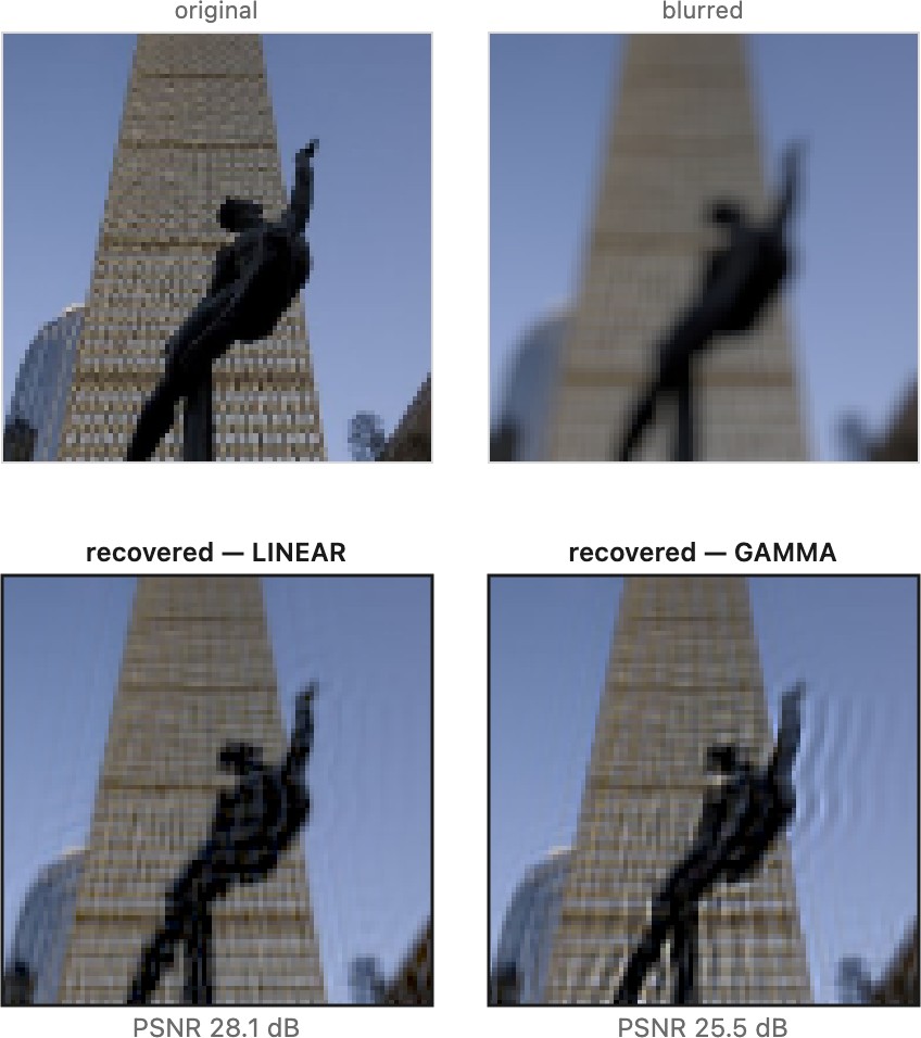
For an ideal power-law encoding $V=L^{1/\gamma}$, an exposure gain $2^{EV}$ becomes $V'=2^{EV/\gamma}V$, and a channel gain $g_c$ becomes $V_c'=g_c^{1/\gamma}V_c$. These identities are exact only for the power-law model before clipping. sRGB has both an offset power segment and a linear toe; use its actual decode and encode functions for an exact adjustment.
Quantization is different: rounding discards information. With code step $\Delta$, nearest rounding has error at most $\Delta/2$ before clipping. Modeling that error as uniform and independent, with variance $\Delta^2/12$, requires sufficiently varying or dithered input; a smooth gradient can instead produce structured banding. Its size relative to shot and read noise depends on gain, bit depth, and processing. Encoding also makes a constant code step correspond to a signal-dependent step in linear light. See Chapter 2.8, Noise, signal-to-noise ratio and dynamic range.
Third, not everything we want is a linear function of the scene. The model $\mathbf{y}=A\mathbf{x}$ recovers the image $\mathbf{x}$ (radiance on a grid), but much of computational photography is after something else entirely: the depth of each pixel, the motion in the frame, the material of a surface, the identity of a face. These are in general not linear read-outs of the light. Depth from defocus or stereo, for instance, enters through a ratio of blurs or a disparity search (a nonlinear estimation, not a matrix inverse) even though the image formation that produced the measurements was perfectly linear. The linear-operator picture governs how light becomes pixels; it does not promise that the thing you actually care about is linearly encoded in them. This is a recurring note of Chapter 5.8, Photographic representation and its limits: a photograph is a flat projection, and the quantities that projection discards, depth above all, must be inferred, not inverted.
Fourth, even where the forward model is linear, two practical gaps open around $A$ itself. Sometimes you simply do not know it: blind deblurring, the bilinear case of Chapter 6.7, Image formation as a linear system, must solve for the operator and the scene together, and is rescued only by priors on both (→ Chapter 16.4, Blind deblurring). More insidiously, sometimes you think you know $A$ but you are wrong: the point-spread function is slightly off, the noise is not quite Gaussian, the optics have drifted. A confident inversion of a subtly mistaken model manufactures confident artifacts, structure that looks real and is not. Robustness to model error is a real and under-appreciated cost of every method that leans hard on knowing $A$.
Fifth, a linear forward model can have either a linear or a nonlinear estimator. Fixed quadratic regularization gives, when the matrix is invertible,
which is linear in the measurement $\mathbf y$. A nonzero prior mean adds an affine offset. Sparsity penalties, positivity constraints, adaptive weights, and learned denoisers generally produce nonlinear estimators. The forward model and the estimator are separate choices (Chapter 7.1, Imaging as Bayesian inference with probabilistic priors).
A differentiable nonlinear forward model $F$ can also be approximated locally by $F(\mathbf x+\delta)\approx F(\mathbf x)+J_F(\mathbf x)\delta$. The Jacobian describes small changes around the current estimate, not a globally linear camera. Clipping has zero derivative beyond saturation; visibility changes and other discontinuities may invalidate this local approximation.
Repeated rounding to a low bit depth and strong shadow lifting make quantization particularly visible. A tone curve can spread a handful of input codes across a broad displayed interval, turning small code steps into bands. Dithering changes the spatial pattern of the error, while retaining adequate precision between operations avoids additional rounding. Neither recovers distinctions already removed by the first quantization.
Image representation⧉
How the array sits in memory⧉
optionalThe array is two- or three-dimensional, but computer memory is one long line of numbered addresses. Something has to decide how the grid gets flattened into that line, and there is no single right answer. Different ecosystems made different choices, which matters the instant you pass an image between them.
The examples use packed planar C++ storage and HWC Python arrays. In contiguous planar storage, the element offset is $cWH+yW+x$; in contiguous interleaved storage, it is $(yW+x)C+c$ (Figure 8.1.6). A NumPy array can have other strides after slicing or transposition, and tensor dimension order does not uniquely determine physical memory layout. Query shape, strides, and contiguity at library boundaries. Row strides are $W$ elements per planar channel or $WC$ elements for interleaved RGB, before padding; byte strides also include element size.
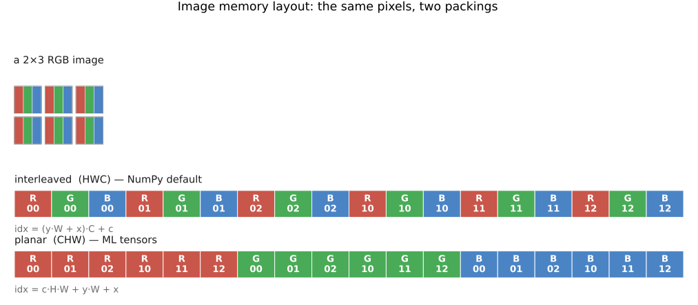
R G B R G B … row by row; pixel $(x, y, c)$ is at offset $(y\cdot W + x)\cdot C + c$. Planar (CHW): all of the red channel, then all of green, then all of blue, three contiguous planes; pixel $(x, y, c)$ is at offset $c\cdot W\cdot H + y\cdot W + x$. Same numbers, same picture; only the walk order through memory differs.The second decision is the order within a pixel. Most of the world, and this book, store the channels as red, green, blue (RGB), but a few libraries, OpenCV being the notorious one, use BGR. Mix the two and red and blue swap silently: skies turn orange, skin turns blue, and nothing throws an error. So always know which order your data is in.
Why care about any of this for everyday code? Mostly you should not. The mental model is just "a grid of pixels," and the accessor we build below hides the packing entirely. Two situations force you to think about it: performance (a loop that strides through memory in contiguous order runs far faster than one that hops around, so the right layout for an algorithm matters when speed does), and interoperability (handing an image to a library that expects a different layout means rearranging the array first). Outside those, the packing is an implementation detail.
Walking contiguous elements usually makes better use of cache lines and vector instructions. For packed HWC data, scalar loops run y, then x, then c; for planar CHW, c, then y, then x. A kernel that processes one whole pixel at once can hide the channel loop. Tiling, vectorization, compiler transformations, and hardware affect the best schedule; measure the implementation (Figure 8.1.7).
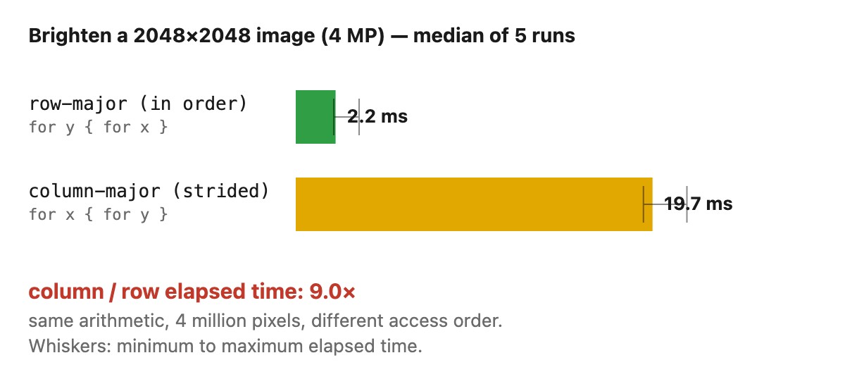
for y { for x } and the cache-hostile for x { for y }, warms up the JIT, then times several passes of each and reports the medians with their min–max spread. The arithmetic and the pixel count are identical; only the memory access order differs, yet the column-major walk typically runs several times slower on the very machine you are reading this on. Interactive: press Run to re-measure, and change the image size; watch the column-major bar stay several times longer than the row-major one, with tight whiskers showing the measurement is stable.Planar storage makes same-channel values contiguous. Interleaving keeps all channels of each pixel together, which can help operations that use them jointly. Vector implementations can handle either layout. Conversion costs and the whole pipeline matter more than declaring one layout universally faster.
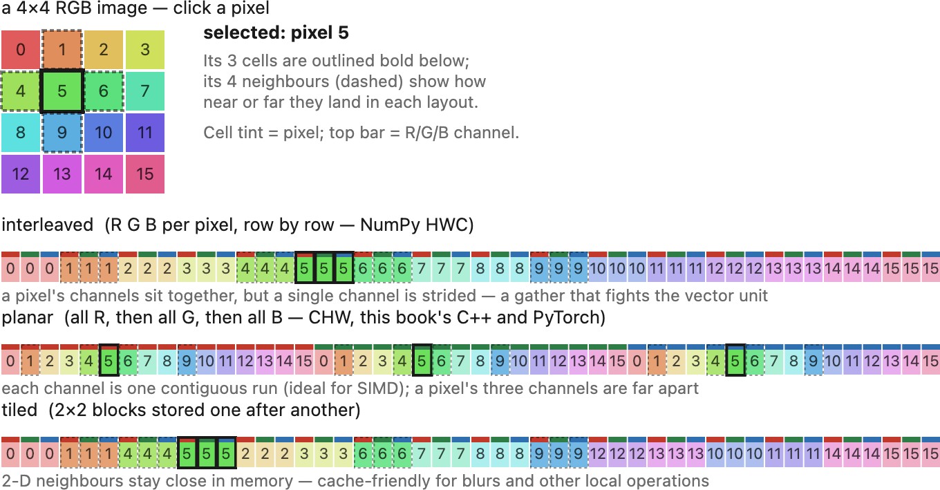
R G B together, row by row), planar (all the reds, then the greens, then the blues), and tiled (small 2×2 blocks laid one after another). To work on one channel, planar storage offers it as one contiguous run, the access a vector unit wants, while interleaving scatters it across every third cell. Tiled storage keeps a pixel's 2-D neighbors close together, which is what a local operation like a blur wants; no layout wins outright, you pick the one your access pattern rewards. Interactive: click a pixel to highlight its cells and its four neighbors across all three layouts, and flip the layout to watch the access pattern change.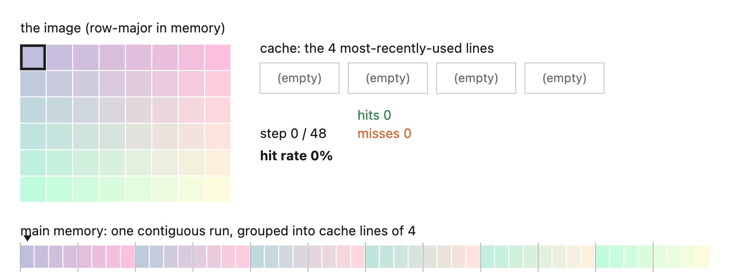
for y { for x } walks memory in order, so each miss loads a line that then serves the next several reads as hits; for x { for y } jumps a full row's stride every step, to a fresh line that is evicted before the loop returns, so almost every read misses. Same pixels, same arithmetic, very different hit rate. (A teaching model, real caches are larger and set-associative, but the locality effect is exactly this.) Interactive: play or single-step, and flip the loop order to watch the hit rate collapse.Prefer traversal that reuses nearby stored values. For scalar loops over packed HWC, use y, x, c order; for packed CHW, use c, y, x. Actual strides, tiling, and vectorized kernels can change the best schedule. Measure before changing the representation.
This book carries a concrete, working C++ image data structure; seeing it once makes the planar arithmetic above concrete. It is deliberately minimal: three integers for the shape, and a single flat buffer of floats in planar order:
struct Image {
    int width, height, channels;
    std::vector<float> data;        // planar: c*width*height + y*width + x

    Image(int w, int h, int c)
        : width(w), height(h), channels(c),
          data(static_cast<size_t>(w) * h * c, 0.0f) {}

    // The accessor: hides the index arithmetic, so the rest of the
    // code can think in plain (x, y, c).
    float& operator()(int x, int y, int c) {
        return data[static_cast<size_t>(c) * width * height + static_cast<size_t>(y) * width + x];
    }
};
This minimal accessor assumes validated nonnegative dimensions, a checked allocation-size product, and in-range indices. Use a sufficiently wide unsigned type for offset multiplication. A production image class also needs const access and explicit boundary reads; an unchecked mutable reference cannot implement zero padding safely. In Python, the book uses arr[y, x, c].
The accessor makes the storage choice concrete without spreading it through the rest of the program. A call such as img(x,y,0)=1.0f looks like indexing a three-dimensional image, while the function computes one offset into the flat buffer. Changing packing later requires changing this mapping and the code at library boundaries, rather than every mathematical expression. Read access beyond an image edge should be a separate policy from obtaining a mutable reference to a stored pixel.
The loop-order effect comes from reuse of fetched data. A cache line brings several neighboring values into the processor together. Traversing a packed row uses those values before moving on; jumping one full row per inner iteration can touch many cache lines while using only one value from each. A different schedule may recover that reuse through tiling or vectorization, which is why the benchmark measures the implemented loop rather than proving a universal ordering rule.
Pixel coordinate conventions⧉
optionalBefore we trust ourselves to index an image, two small geometric conventions have to be nailed down, because both are silent traps and both differ between tools.
The first is where the origin sits. We place $(0, 0)$ at the top-left pixel, with $x$ increasing to the right and $y$ increasing downward: the order in which image data is scanned and stored, and the convention most imaging code (and our own camera frame) uses. The catch: a few systems (classic OpenGL textures, and much plotting and math software) put the origin at the bottom-left, with $y$ increasing upward, as on a graph. Hand an image from one world to the other without flipping it and the picture comes out upside down (Figure 8.1.10). Nothing crashes; it merely looks wrong, which is the worst kind of bug to chase.
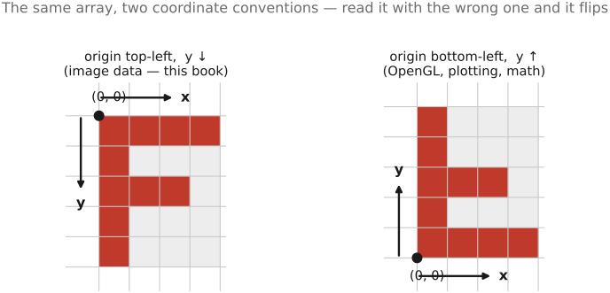
We assign integer coordinates to pixel centers. A displayed pixel cell at $(0,0)$ spans $[-0.5,0.5)$ along each axis, and the image footprint spans $[-0.5,W-0.5)\times[-0.5,H-0.5)$. This geometric cell convention does not assert a box-shaped sensor response. APIs that place integer coordinates at cell corners differ by half a pixel.
That half-pixel sounds pedantic, and for a point operation it is: a curve applied to every pixel never asks where a pixel is. But the moment you resample or warp (scale up, rotate, correct lens distortion) you are evaluating the image at non-integer positions, and a consistent half-pixel error shifts the whole result by half a pixel, blurs it, or makes a "round trip" (shrink then enlarge) fail to land back where it started. It is one of the most common bugs in resampling code precisely because it never raises an error. We fix the convention now (integer = center) and return to it in full at resampling and warping, where it earns its own discussion of "where-from vs. where-to" addressing.
Keep two facts straight and most coordinate bugs evaporate: the origin is top-left, $y$ down, and an integer coordinate names a pixel's center, not its corner. Both are conventions, not laws: other tools choose differently, so check before you trust.
Pixel lookups and boundaries⧉
Almost every operation in the coming chapters reaches for a pixel's neighbors, which forces an unavoidable question: what is $I(x, y)$ when $(x, y)$ lands outside the image? We cannot dodge it, because blurs, gradients, resampling, and warps all ask for out-of-bounds pixels right at the border, where there are no neighbors on one side. Reading past the array is, at best, garbage and, at worst, a crash, so the first discipline is defensive: route every pixel read through a single accessor function, a small get(x, y, c), so that out-of-bounds access is decided in exactly one place rather than re-improvised (and re-broken) in every loop. As a bonus, that one function is also where the memory layout, the channel order, and the coordinate convention live, so the rest of the code can think in plain $(x, y, c)$ and forget every packing decision above. It is the natural home for one more safety check, too: asserting that an index lies in $[0, \text{size})$ inside that single function turns a distant, hard-to-trace crash into an immediate, localized error (we develop this habit in the debugging chapter).
The accessor then has to decide what a pixel past the boundary means. There are four standard policies (Figure 8.1.11):
- black / zero: treat everything outside as $0$. Simple, but it darkens edges, since you are averaging in black that is not really there.
- clamp / replicate: repeat the nearest edge pixel outward. A reasonable, neutral default for many operations.
- mirror / reflect: fold the image back across its boundary, so the neighborhood just past the edge mirrors the one just inside. This avoids both the artificial darkening of zero and the streaking of clamp, and is the usual safe default for filtering.
- wrap / tile: treat the image as periodic, the left edge adjacent to the right. Rarely what you want visually, but it is exactly the assumption the Fourier transform makes, so it returns when we get there.
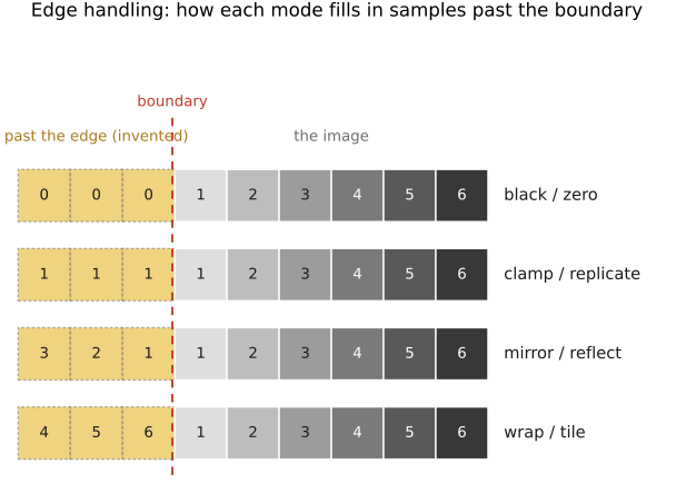
On a real photograph the four policies look like Figure 8.1.12: the same crop, continued past its border each way, surrounded by a dark frame, streaked outward, folded back on itself, or wrapped around from the opposite edge.
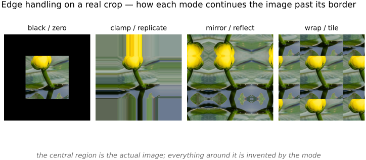
The boundary rule changes filtering and resampling near the border. We use reflection for these examples, stating whether the edge sample is repeated: libraries distinguish whole-sample and half-sample reflection. Neither reconstructs unseen content. For inverse problems, the adjoint must include the selected extension rule; see Chapter 6.9, Efficient linear solvers.
Three kinds of operation⧉
optionalThe domain/range split we just drew also sorts everything we will do to an image into three families, each the basis of one of the next several chapters (Figure 8.1.13):
- point operations touch the range only: a pixel's new value depends solely on its old value, the same rule applied everywhere (brightness, contrast, tone curves, gamma);
- domain operations change spatial coordinates; interpolation may also change values: each output pixel pulls its value from a different input location (translation, rotation, resizing, lens correction);
- neighborhood operations compute each pixel from a window of its neighbors (blur, sharpen, edge detection).
This is a preview; each family gets its own development later (point operations come first). But the taxonomy already earns its keep, because it predicts cost: a point operation reads each pixel once, while a neighborhood operation reads many input pixels per output pixel. We will flag which family every new tool belongs to as we go.
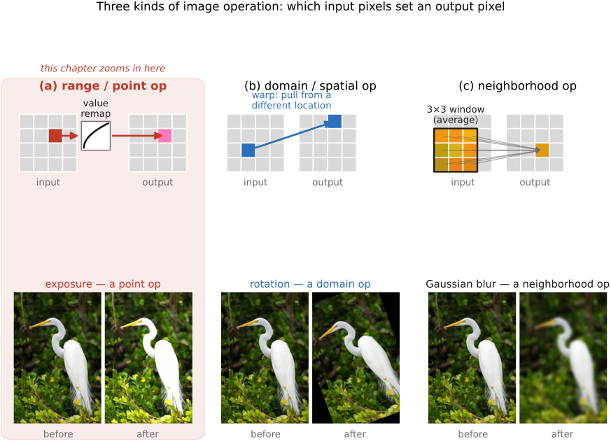
Sharpening⧉
PS2 implements box/Gaussian blur, gradients, sharpening, and the bilateral filter. → Chapter 1.5, Problem sets (appendix).
Sharpening increases contrast around edges and texture. The common unsharp mask extracts a blur residual and adds some of it to the image. It enhances detail that survived capture; it does not invert the imaging process. Chapter 16.2, Non-blind deconvolution treats reconstruction from a blur model.
Linear sharpening⧉
The linear core of sharpening was built in Chapter 6.2, Convolution: blur the image to get its slow, smooth part, subtract that to isolate the fine detail the blur threw away, then add the detail back amplified. That is the unsharp mask,
with $k$ setting the strength: flat regions have near-zero detail and are left alone, while edges and texture gain contrast. Push $k$ too high and it over-sharpens.
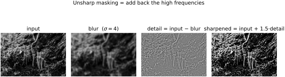
Because each step is linear, the whole operation collapses to a single convolution, $I_\text{out} = I * \big(\delta + k(\delta - g)\big)$: a positive spike at the center ringed by a negative surround. Chapter 6.2, Convolution traces that center-positive, surround-negative signature across the unsharp mask, the Laplacian, and the difference of Gaussians, and shows why they are one family.
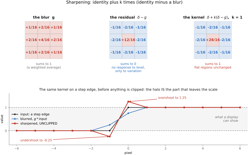
The blur radius selects the scale of detail being enhanced, while $k$ selects its strength. A larger radius makes wider halos. Judge sharpening after resizing for the intended output, since changing image size changes the meaning of a radius in pixels.
Why it's called "unsharp mask"⧉
optionalThe name is a darkroom relic; it explains the otherwise puzzling word unsharp in a sharpening tool. Before digital, photographers sharpened a negative by sandwiching it with a slightly blurred, low-contrast positive copy (an "unsharp mask") held a hair out of focus against the original. The positive mask opposes the negative’s broad density variations while leaving the finer transitions relatively stronger. Optical densities add in the sandwich, so this is an analogy to residual enhancement in a density-like domain, rather than literal subtraction of linear pixel values. The blurred copy is the “unsharp” mask, and its name survived the move to digital processing. The effect can be simulated in density (Figure 8.8.3).
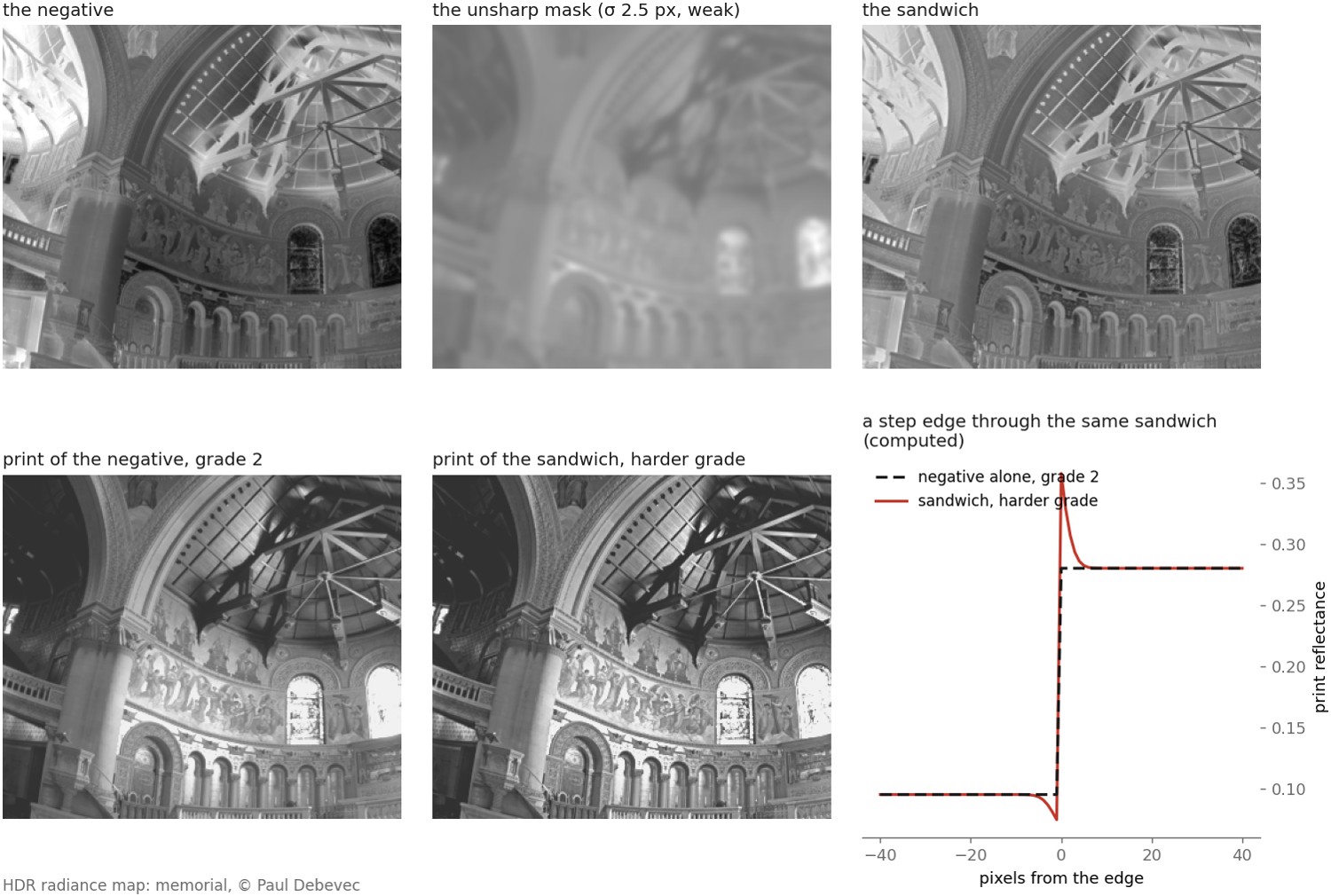
Sharpen in gamma, linear, or log?⧉
optionalThere is another choice in that formula that most people never make consciously: in what space do you compute the subtraction? The unsharp mask is a weighted difference (original minus a blur) and a blur is an average. We already know from tone mapping and from color that an average depends on the space you take it in: the mean of two pixels is not the same number in gamma-encoded values, in linear scene radiance, and in log. So the same unsharp mask, with the same radius and strength, gives three different results depending on whether you apply it to the encoded values in a rendered file, to the linear light those values decode to, or to the log of that light.
The encoding changes both the blur and the residual. A linear unsharp mask gives equal and opposite numerical overshoots around an ideal step before clipping; they need not look equally strong after display encoding. In log luminance the changes are multiplicative after exponentiation. No domain makes sharpening an exact physical reconstruction. State the encoding, keep intermediate headroom, and inspect both sides of strong edges.
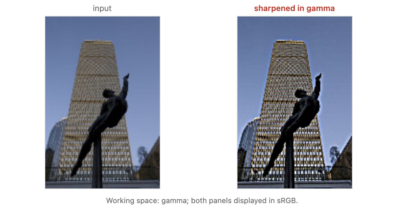
Non-linear sharpening⧉
optionalLinear unsharp masking is the standard sharpen, and it has two failure modes that motivate everything left in this chapter.
First, it amplifies noise. In a flat region (a clear sky, a smooth wall) there is no real detail, so $\text{in} - \text{blur}$ is mostly noise. Boost it and you boost the noise, turning a clean sky grainy. Second, it haloes at strong edges. Near a high-contrast boundary the detail image swings strongly positive on the bright side and negative on the dark side; amplify that and you get a bright fringe along one side of the edge and a dark fringe along the other, the tell-tale "halo" of an over-sharpened photo. Both failures appear on a real photo as the gain $k$ is pushed up (Figure 8.8.5): a scanline across a strong edge shows the boosted detail overshooting into a bright/dark ring, while the smooth background turns gritty.
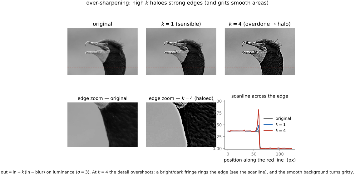
Linear sharpening uses the same gain on noise, texture, and strong boundaries. Adaptive variants reduce the gain where the residual is small or where an edge would overshoot [@ramponi-1998; @polesel-etal-2000]. A threshold is only a heuristic: faint texture can fall below it, and large noise can exceed it. Luminance-oriented sharpening limits color fringes, while a local output bound can limit overshoot.
A simple residual gate can be written as pseudocode:
b = blur(I, radius)
d = I - b
detail = sign(d) * max(abs(d) - threshold, 0)
out = I + amount * detail
# Optional: bound out by local input extrema to limit overshoot.
This soft threshold avoids a jump at the threshold, but removes some weak detail along with noise. A local bound is another nonlinear choice and can flatten peaks.
The fastest way to feel both the linear failure and its non-linear fixes is to drive them, watching a scanline through the image (Figure 8.8.6).
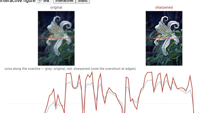
Content-dependent weights make a filter nonlinear. This differs from a fixed convolution, but does not necessarily break translation equivariance: translating the input can still translate the output. Chapter 10.1, Bilateral filtering develops one such neighborhood rule.
Learned enhancement can also synthesize plausible texture where the measurements are ambiguous. A sharper-looking result does not establish that the detail was recorded; see Chapter 14.1, What can super-resolution actually do?.
The Detail panel of Chapter 8.13, A raw developer in the browser is this chapter's shrink-then-sharpen in a single pass, with the luminance/chroma split and the edge mask as written here.
An unsharp mask amplifies whatever high-frequency residual it receives. That residual can be a real texture, sensor noise, ringing from compression, or a demosaicking artifact. A threshold can suppress small residuals, but a faint real texture may be small too. A local strength map can reduce the boost in smooth regions and preserve stronger detail elsewhere. Inspect both a smooth patch and an edge when tuning it: an image can look crisper overall while acquiring conspicuous noise or halos in particular regions.
Spatially varying blur⧉
A table of blurs, and which are convolutions⧉
optionalSummarize the blurs in one place, because the single most consequential property of any blur is whether it is shift-invariant (one kernel convolved everywhere, the only case the FFT/Wiener machinery handles directly) or spatially varying, where it is not a convolution at all. With Oliver Whyte's camera-shake model as the centerpiece, the catalog is:
| blur source | physical cause | shift-invariant? |
|---|---|---|
| Translational camera motion | the camera slides sideways during the exposure | approximately for constant depth and suitable motion; depth variation causes parallax |
| Camera shake (rotation) | wrist pitch/yaw, the dominant hand tremor | generally spatially varying; pure roll has a stationary center (Whyte et al. 2011/2014) |
| Defocus | a point's depth differs from the focus plane | approximately uniform on a single depth plane; varying depth and occlusion require more |
| Subject / object motion | something in the scene moves while the camera is still | no, only the moving region blurs, each along its own path |
| Lens aberrations | imperfect optics: coma, astigmatism, field curvature | no, mild on-axis, worse toward the field edge; per-channel for chromatic aberration |
| Atmospheric turbulence | hot air, long lenses | no, a shimmering warp that varies in space and time |
Whether convolution is adequate depends on the scene and regime. A frontoparallel constant-depth plane under lateral translation can give a uniform motion blur; one defocus depth with approximately field-invariant optics can also give a convolution. General 3-D translation, varying depth and visibility require more.
Algorithmic speedups⧉
Separability: a 2-D pass for the price of two 1-D passes⧉
optionalA separable kernel factors as $K(u,v)=h(u)g(v)$. Substitution gives
Compute the bracketed horizontal filter first, then filter its result vertically. The work per output falls from $(2k+1)^2$ weighted contributions to $2(2k+1)$. For a $25\times25$ kernel, that is 625 versus 50. Equality assumes the same kernel and compatible boundary extension; floating-point rounding can still differ.
The second pass introduces an intermediate and its memory traffic. A vertical stencil is not automatically contiguous in a row-major image, although processing adjacent output columns allows reuse and vectorization. Tiling and fusion determine how much of the arithmetic saving survives on the machine.
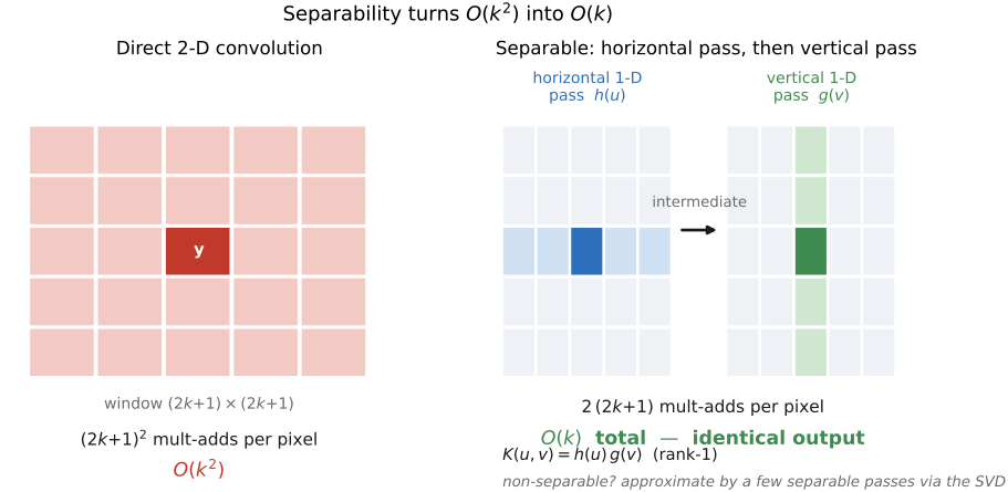
For a nonseparable kernel, its singular value decomposition gives a sum of separable terms. Retaining a few terms approximates the kernel with a corresponding error. Compare the resulting images as well as the kernel norm; see Chapter 6.2, Convolution.
The next accelerations share another form of reuse. A running sum retains what overlaps between successive windows. A prefix table retains cumulative sums for later rectangle queries. A sliding histogram retains counts so the next median need not start from a new sort. Each chooses a state that can be updated more cheaply than recomputing the answer from its definition.
Recap: big lessons in this lecture
We will lean almost entirely on ray (geometric) optics, because nearly every source and interaction we meet is incoherent, and incoherent imaging is linear in intensity. The one piece of the wave picture we hold onto is that the physical color of light is its spectral distribution, the energy it carries at each wavelength. The exceptions to the ray picture are narrow: light squeezed through a small hole (diffraction), a thin film (interference), or a fine structure (structural color), and even structural color we can usually fold into absorption and go on treating the light as rays. Ray optics and incoherent imaging are linear, with one standing catch: the quantities are always positive, so we can add light but never subtract it. Coherent light and full wave optics, where amplitudes add and can cancel, come back only for the advanced topics of metalenses, lensless cameras, and holography, and the particle picture we keep mostly for modeling noise. So most of the time we will picture light as a set of rays traveling in straight lines through homogeneous media, each carrying a radiance that is itself a distribution over wavelength. With that, we have followed light from its source, off a surface, and to the edge of the camera; the chapters that follow take up how eye and camera turn that light into color and into an image.
Counter to ray-optics intuition, a smaller aperture spreads light more: the diffraction blur (the Airy disk) grows as $\sim\!\lambda N$ with f-number, so stopping down past a point softens the image instead of sharpening it. The flip side is the rule behind every instrument that must resolve fine detail: only a large aperture can diffract little and resolve finely, which is exactly why microscopes and telescopes are built around large lenses and mirrors, and why a phone camera's tiny aperture hits a hard resolution wall it cannot pass. It is the optical cousin of "you can't sample your way past Nyquist."
Camera rotation (yaw/pitch) smears the image by $b_{\text{px}} \approx f_{\text{px}}\,\theta$, the same for every object regardless of depth. Camera translation and subject motion smear it by $b_{\text{px}} \approx f_{\text{px}}\,(\Delta \text{ or } v\Delta t)/D$, which shrinks with distance. So for ordinary distances rotation dominates, and only up close (macro) does translation take over. The focal-length dependence divides the same way: yaw and pitch blur scale with $f_{\text{px}}$, so a longer lens (higher magnification) turns the same angular wobble into proportionally more blur (the basis of the $1/f$ hand-holding rule), while roll blur $b \approx r\,\theta_{\text{roll}}$ is fixed by image position $r$, not by focal length. Magnification amplifies yaw and pitch but never roll, which is why yaw and pitch usually dominate the shake blur, the more so the longer the lens. And because roll and perspective make $b$ vary across the frame, camera-shake blur is spatially non-uniform: a single blur kernel cannot describe or undo it.
Reflected ambient light raises the visible black level. Prepare and judge the image under its intended viewing conditions; a panel specification alone does not describe the contrast the viewer will see.
An operation $F$ is linear when $F(a x+b x')=aF(x)+bF(x')$. For finite sampled signals, each output is a weighted sum of inputs with weights independent of the data. Stacking those weights into rows gives $y=Ax$. The matrix describes the operation; code can apply its weights without allocating the matrix.
A convolution uses fixed weights that depend on displacement, not on image values or absolute position. On an infinite or periodic grid it is linear and commutes with shifts. The kernel can be small or span the image. Its support determines the work of direct filtering; finite boundaries determine where the shift-invariance model applies.
Convolution can be computed per output pixel or per kernel tap. In the first order we accumulate a neighborhood; in the second we accumulate shifted copies of the image. The result is the same. Replacing shifts with known warps gives other linear operators, but they need not share convolution’s commutativity or Fourier diagonalization.
Finite differences are convolutions with signed kernels under a declared indexing convention. In the continuous setting, $\partial_x(g*I)=(\partial_x g)*I$: convolving with a derivative-of-Gaussian differentiates a smoothed image. Gradient components are linear; gradient magnitude, thresholding, and a complete edge detector generally are not.
A convolution is an approximation when blur changes with depth, motion, field position, or wavelength. A small patch may support one kernel, but occlusion boundaries need particular care. Fixing geometry can preserve linearity in intensity even when shift-invariance is lost.
Express a linear operator in a basis where it becomes diagonal. A coupled, hard-to-invert operation in one representation can be a list of independent scalar multiplications in another, and scalars are trivial to understand, compose, and invert. Fourier diagonalizes convolution, turning a blur into per-frequency multiplication. This is not a one-off trick: it is the single most reusable move in applied linear algebra, and it returns for differential equations (the heat equation, below), for principal components, and for nearly every inverse problem in this book. The idea is already visible in the smallest possible case, a $2\times2$ matrix (Figure 6.3.3).
Phase specifies the alignment of the waves; magnitude specifies their strength. Phase swaps between typical photographs often preserve recognizable structure from the phase donor, but accurate reconstruction requires both.
Natural photographs often have approximately $1/f$ average Fourier amplitude over a range of scales. Distinguish amplitude from power, and average power per coefficient from total energy in a frequency band. The image mean can dominate total energy without explaining its visible detail.
In the Fourier basis a convolution is diagonal: it multiplies each frequency by one number (the kernel's complex response, the OTF), so undoing it is a per-frequency division. The whole stability question becomes local to each frequency: how near zero is that number? Blur is low-pass, so its response is tiny at exactly the high frequencies it destroyed; the lower a frequency's coefficient, the more its noise is amplified on inversion. That is why naive deblurring fails worst precisely where the blur was strongest, and why a Wiener / regularized filter stops dividing once the signal drops below the noise floor.
Recovery depends on which variations the operator measures, their signal-to-noise ratios, and how accurately the operator is known. A null space leaves ambiguity; small gains make inversion sensitive to noise. An unknown or miscalibrated operator adds a separate estimation problem.
Prefer traversal that reuses nearby stored values. For scalar loops over packed HWC, use y, x, c order; for packed CHW, use c, y, x. Actual strides, tiling, and vectorized kernels can change the best schedule. Measure before changing the representation.