💬Comments welcome. To leave a note, select any text and click the note / highlight button that pops up — or open the panel with the tab at the top-right (‹). Notes are visible only inside our private review group.
Course notes cut from Computational Photography, an AI-powered Slopendium for this lecture. Each section links back to its home in the book; sections marked optional go beyond what the lecture needs.
Contents · 61 sections on this page, from 38 chapters of the book
Python is a convenient default for numerical experiments. NumPy represents images as arrays, while PyTorch and JAX add GPU computation and automatic differentiation. A per-pixel loop in Python can be slow; an array expression delegates the loop to compiled code. Vectorization can also create large temporary arrays, so memory traffic still matters. In conventional CPython builds, the global interpreter lock limits simultaneous execution of Python bytecode; compiled libraries can release it, and optional free-threaded builds have different behavior. Check the interpreter and extensions you deploy (Python documentation).
C++ offers explicit control of data layout, allocation, and parallel execution. That is useful for a pipeline with a tight latency or memory budget, but it requires more care with indexing, ownership, and build configuration. Standard containers and resource-owning objects reduce the need for manual allocation. Static types catch some errors; they do not catch a wrong color space or an out-of-bounds access automatically.
Halide separates an image-processing algorithm from its schedule: where and in what order values are computed, stored, vectorized, and parallelized. This lets the same algorithm support several execution strategies without rewriting its mathematical definition. Good schedules can avoid intermediate images and repeated memory transfers. They do not guarantee a fixed speedup over well-optimized C++ (Halide).
Sidebar 1: Photoshop's early language split
In 2013 Adobe, through the Computer History Museum, released the source of Photoshop 1.0.1: about 128,000 lines in 179 files, written for the original Macintosh largely by Thomas Knoll. Roughly three quarters is Pascal, the productive high-level language for the bulk of the program, and about 15% is hand-written 68000 assembly for the speed-critical inner loops. That is the split this chapter keeps returning to, thirty-five years early: hand-tune the hot pixel loops and keep the rest readable, the same trade as Python calling a compiled library, with a person doing by hand what Halide now automates. The code is now read as a cultural text too: the German research program Das digitale Bild (DFG, LMU Munich) has published a critical code study, reading the Photoshop source the way one close-reads a document (Reading the source code for Adobe Photoshop). The appendix runs the program itself (Chapter 45.33, Photoshop 1.0, running), and Part 29, Making computational photography code fast returns to hand-tuned inner loops.
Much of the computational-photography literature was prototyped in MATLAB. For years it was the platform for this kind of work: a strong numerical and linear-algebra library, and an interactive IDE that could read, display, and manipulate images natively: an image was just a matrix, imread/imshow and array slicing made experiments effortless, and the Image Processing Toolbox supplied the rest. NumPy carries the same array-as-image approach into Python, while frameworks such as PyTorch combine tensor operations with automatic differentiation and GPU execution. We mention it because older papers and code you will meet are written in it, and the array-thinking it taught carries over directly to NumPy. Choose the environment that lets you reproduce and inspect a method, rather than translating working research code only for consistency of language.
For example, NumPy's out = a + 0.5*b makes a point operation almost as direct to write as its mathematical definition. That short edit-and-run cycle matters when the algorithm itself is uncertain. Once the operation is settled, C++ can give more control over storage and execution, with a heavier build cycle and more responsibility for object lifetimes. Halide adds a scheduling language when the performance question is where to compute and retain intermediate values. These are different costs to pay at different stages of a project.
Implementing a method exposes choices that an explanation can hide: boundary handling, units, numerical precision, and failure cases. These assignments from MIT's Digital & Computational Photography course ask you to build simplified algorithms and try them on real photographs. Their sequence follows the course rather than the book; each assignment links to the chapters it uses. Full handouts are collected in Part 45, Appendices.
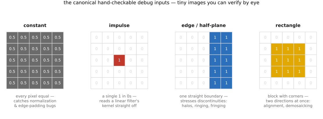
Start with small inputs you can check by hand, then inspect the photographic results. A constant image, an impulse, or a known geometric transform often reveals an error more clearly than a natural photograph. If you are taking a course, follow its own submission and AI-assistance rules.
PS3: Denoising and demosaicking. Align-and-average a burst (and the ISO/variance story); Bayer demosaicking: basic green, then edge-directed green and color-difference R/B; and Prokudin-Gorsky three-plate color alignment. (→ Part 13, Denoising, Part 15, Demosaicking and joint methods)
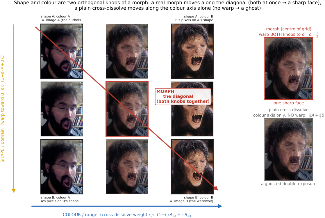
PS5: Resampling, warping, and morphing. Nearest / bilinear / bicubic / Lanczos resampling; Beier–Neely segment warps; and a full Beier–Neely morph. (→ Chapter 11.1, Warping, Chapter 11.3, Morphing)
PS6: Homographies and manual panoramas. Homogeneous coordinates, warping by a homography, solving the homography from four point correspondences, and stitching a planar mosaic. (→ Chapter 20.1, Manual panorama stitching from multiple views)
The assignments deliberately distill an area into a small algorithm that you can build and inspect. Their purpose is to expose the principle before the production machinery obscures it. A basic align-and-average burst, for example, makes registration and noise reduction visible even though a shipping camera will need more elaborate handling of motion and outliers.
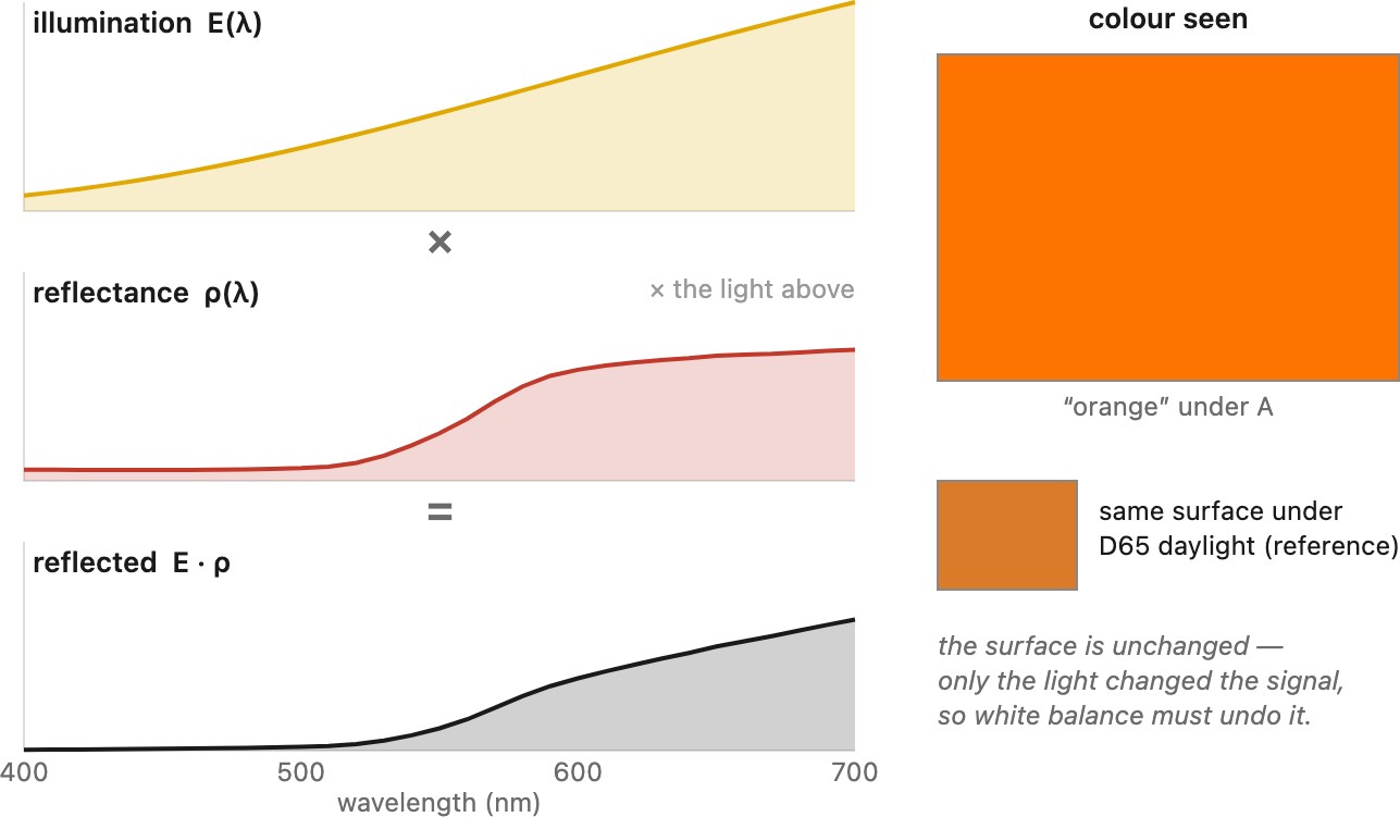
Most ordinary photographed objects emit negligible visible light of their own; they only reflect whatever light falls on them. So the color that reaches your eye is the result of two spectra multiplied together, wavelength by wavelength:
$$ C(\lambda) = S(\lambda)\,\rho(\lambda). $$
Here $S(\lambda)$ is the illuminant (the spectrum of the light source actually present) and $\rho(\lambda)$ is the surface's spectral reflectance, the fraction of light it sends back at each wavelength. Reflectance is the object's intrinsic, fixed signature: the apple's $\rho(\lambda)$ is high in the reds and low in the greens and blues, whatever the lighting. Illumination is whatever happens to be shining. Their per-wavelength product is what leaves the surface and reaches the eye (Figure 2.1.28). A red apple under white light reflects mostly red; the same apple under pure green light has almost nothing to reflect and looks nearly black, because there is no red illumination for its reflectance to act on.
Figure 2.1.28(reproduced). Color is illumination × reflectance. A surface's fixed reflectance spectrum ρ(λ) (here an apple's, high in the reds) is multiplied per wavelength by the illuminant spectrum S(λ) actually present. The product C(λ) = S(λ)·ρ(λ) is the light that reaches the eye. Change the illuminant and the product changes even though the surface has not: the same reflectance under white versus reddish versus greenish light yields three different stimuli. One swatch shows the surface's unadapted appearance under the chosen illuminant; a smaller reference swatch shows it under D65 for comparison.
This multiplicative entanglement is consequential, and it is the first instance of a principle that runs through the whole book.
💡 Big lesson (L2.6) — the multiplicative world
Much of imaging is multiplicative, not additive. The light reaching the eye is illumination times reflectance; contrast is a ratio of intensities; a shadow darkens a region by a factor, not by subtracting a constant. Because the structure is multiplicative, the natural tools are multiply, divide, and log, not just add. This is why, again and again, we will work with ratios and with logarithmic encodings rather than raw linear values. It is also why white balance is hard: to recover an object's true color we must divide out the unknown illuminant $S(\lambda)$ from the product $C(\lambda)$, undoing a multiplication we never observed directly. (The additive counterpoint, light from different sources adding, and what it means for choosing an encoding, comes in Color technology.)
Why this multiplicative structure matters so much is a question the rest of the book keeps answering. Our visual system does not care about the illumination for its own sake. It cares about objects, about the reflectance $\rho(\lambda)$ that tells it what a thing is and whether it is food, a face, or a threat. So the brain works hard to discount the illuminant, factoring the product $C(\lambda)=S(\lambda)\,\rho(\lambda)$ back apart to recover the reflectance and hold an object's apparent color and lightness steady as the light changes. That discounting is the perceptual machinery of lightness and color constancy, studied in Human vision and color, and a camera has to imitate it deliberately, which is exactly what white balance does. Much of imaging is this running effort to see past the illumination to the reflectance underneath.
Image measurements as integrals over the plenoptic function⧉
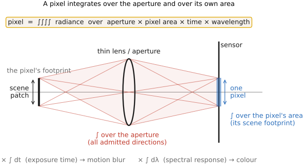
A pixel does not sample a single ray; it integrates over four groups of variables, each weighted by how the pixel responds there (Figure 2.4.2):
the aperture: all the ray directions $(\theta, \phi)$ the lens admits toward this pixel, a solid angle set by the f-number;
the pixel's area $(x, y)$ on the sensor, a finite patch, not a mathematical point;
wavelength $\lambda$, weighted by the sensor's and color filter's spectral response; and
the exposure time $t$, the interval the shutter is open.
The spectral axis, $\lambda$, is the one this book develops furthest elsewhere: collapsing a whole spectrum onto a few numbers weighted by $r(\lambda)$ is exactly where color is born, and how a sensor is built to make that measurement in three or more channels, together with what the resulting numbers mean perceptually, is the subject of Part 3, Visual perception and color and Part 4, Color spaces and color technology, and in particular the chapter on Chapter 4.6, Sensing color: multiplexing strategies. Here we treat $\lambda$ simply as one more axis the pixel integrates over.
the scene radiance integrated over aperture × pixel area × wavelength × time, weighted by the pixel's spectral response $r(\lambda)$ and the geometric weight $k$ that the aperture and footprint impose. Measurement is integrating the plenoptic function against the pixel's sampling kernel, and the support of that kernel along each axis is exactly a photographic knob. Because the underlying capture counts photons, this integral is linear in scene radiance, a fact we will need both for high-dynamic-range merging and for the noise analysis in Chapter 2.8, Noise, signal-to-noise ratio and dynamic range.
💡 Big lesson (L2.26) — a pixel value is an integral
No pixel measures "the" value at a point in space, time, or color: it reports an integral over everything the photosite cannot tell apart. Four axes appear explicitly above: the spatial footprint (the pixel's area, plus the optical blur smeared across it), the exposure time (a window, not an instant), the spectrum (wavelength, weighted by the channel's spectral sensitivity), and the solid angle of rays the aperture admits; a fifth, polarization, is usually lumped in too. Naming all the axes at once is what makes motion blur, defocus, color, vignetting, and aliasing the same phenomenon (a finite integral standing in for an idealized point sample), and the width of the integral along each axis is a knob the rest of the book spends its time controlling.
Figure 2.4.2(reproduced). A pixel value as a four-dimensional integral, a measured slice of the plenoptic function. The thin lens (drawn as an ellipse) admits a cone of rays; the value recorded at one finite-area pixel is the scene radiance integrated over (1) the aperture (which rays/directions the lens admits), (2) the pixel's area on the sensor, (3) wavelength (the spectral response), and (4) the exposure time. Aperture → depth of field; pixel area → sampling/antialiasing; time → motion blur; wavelength → color.
The four domains are the four knobs. This matters because each integration domain is governed by a control the photographer actually sets: the integral is the camera's exposure settings, written as mathematics:
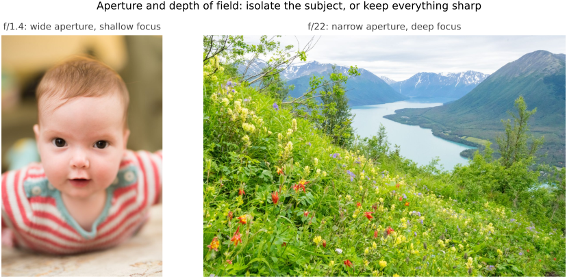
the aperture integral is set by the f-number $N = f/D$: stopping down shrinks the cone of directions each pixel sums over (less light, more depth of field); opening up widens it;
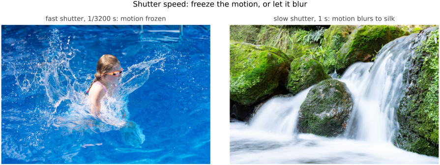
the exposure-time integral is set by the shutter speed: a longer interval integrates over more time (more light, but more motion blur);
the pixel-area integral is fixed by the sensor's pixel pitch (the physical size of a photosite) so larger photosites collect more photons at equal sensor irradiance and exposure, while larger sensor area does not by itself imply larger pixels;
the wavelength integral is shaped by the spectral response (the sensor's sensitivity curve times the color filter over each photosite) which collapses a whole spectrum into a single number per channel.
The one familiar exposure control missing from this list is ISO, and the omission is instructive: ISO is not an integration limit. It scales the result of the integral after the light is collected (analog or digital gain), rather than changing how much light is gathered, which is exactly why pushing ISO amplifies noise along with signal, as the noise section will show.
The deeper reason to write capture this way is that each of the four integration domains earns its own topic later, and much of photography is the craft of choosing how to shape these four integrals. Every later sensing topic is just what happens when you change the support of one axis:
integrating over the aperture is what produces depth of field (the lens chapter): a wide aperture integrates over a fat cone of directions, so an out-of-focus point spreads its energy across many pixels: the circle of confusion. The light-versus-blur trade lives entirely on this one axis;
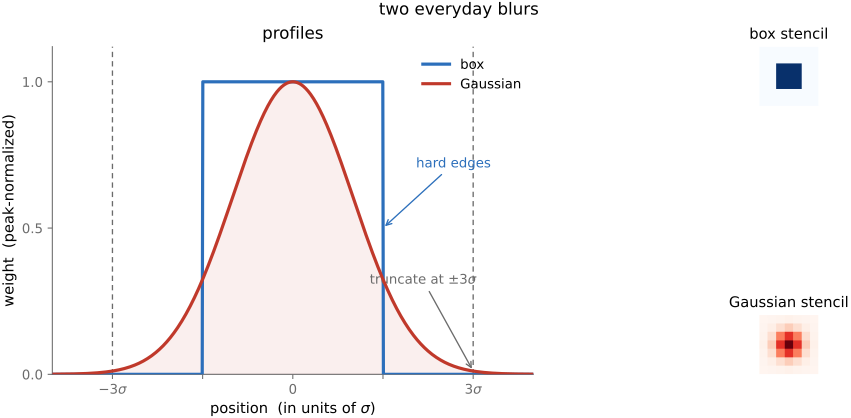
integrating over the pixel's area is sampling and antialiasing (Basic Image Processing): a finite footprint makes each sample a box-filtered average rather than a point sample, pre-blurring the image before it is laid on the grid: a wider footprint suppresses aliasing at the cost of resolution;
integrating over time is motion blur (Motion/Video): a long exposure sums a moving scene over the interval, the temporal sibling of the aperture, trading light against sharpness;
integrating over wavelength is color sensing: the spectral response collapses a whole spectrum into one number per channel, exactly as a cone does (Chapter 3.2, Perceptual color and trichromatic vision). Because a color-filter array gives each photosite a different $r(\lambda)$, color is spatially multiplexed across the Bayer mosaic and must be reconstructed by demosaicking.
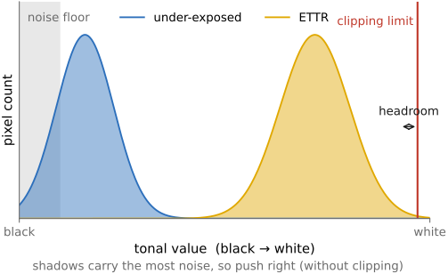
The rest of the sensing story reduces to one question, which kernel, how wide, and what does it lose: antialiasing widens the spatial kernel, depth of field is the aperture kernel, motion blur is the time kernel, and demosaicking inverts the wavelength multiplexing. Each is also a source of noise: a narrower kernel along any axis (a smaller footprint, a shorter exposure, a stopped-down aperture) integrates fewer photons, and fewer photons mean a noisier estimate, which is exactly where Chapter 2.8, Noise, signal-to-noise ratio and dynamic range picks up.
All four axes are then summed into one number: the conventional sensor couples them, discarding how the light was distributed across directions, area, color and time alike. The ideal sensor would do the opposite: decouple the axes, measuring each one separately so we could decide after the shot how to combine them. Chasing that decoupling is a whole branch of computational photography, which the end of the chapter frames.
Framed this way, the measurement integral is a general language for imaging. Every imaging system, from a pinhole to a light-field camera, is described by which weighting it applies to the plenoptic function before integrating: the choice of weights over direction, area, wavelength, and time is the design of the system. And because integration is linear, every such system is a linear operator on the plenoptic function, the viewpoint that Chapter 6.7, Image formation as a linear system develops in full.
For the sake of simplicity, we routinely speak of imaging in terms of infinitesimal quantities: a pinhole that admits a single ray, an exposure that freezes an instant, a pixel that samples a point, a single wavelength of light. These idealizations keep the geometry clean and the diagrams legible. But no real measurement is infinitesimal. A sensor reports a number only by integrating over a finite aperture, a finite area, a band of wavelengths, and a stretch of time, because every axis of the plenoptic function must be summed over to gather enough photons to register at all. The idealized ray and the frozen instant are the limit the mathematics reaches for; the finite integral is what the camera actually delivers, and the gap between the two is where depth of field, motion blur, color mixing, and noise all live.
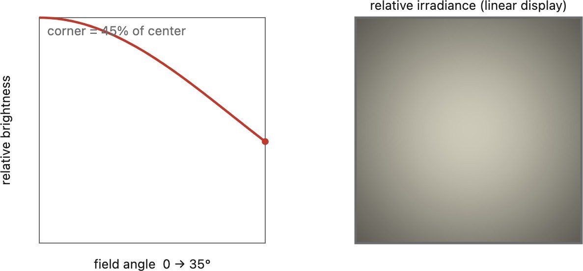
Off-axis ($\cos^4$) falloff. One prediction falls out of this irradiance integral. Rays reaching the corners of the frame arrive obliquely, so the same scene radiance delivers less irradiance there: the aperture-and-area geometry of the pixel integral works out to a $\cos^4\theta$ dimming toward the edges, called natural vignetting (Figure 2.4.3). It is distinct from optical vignetting (lens elements physically blocking edge rays, covered in Optics) in that natural vignetting is a clean consequence of the pixel-integral geometry alone.
Figure 2.4.3(reproduced). Natural vignetting: the $\cos^4\theta$ falloff. Relative pixel irradiance is plotted against the off-axis angle $\theta$, beside a preview of a frame darkening toward its corners. Even with uniform scene radiance, corner pixels receive less light, falling as $\cos^4\theta$, the combined effect of oblique incidence, the foreshortened aperture, and the longer path to the corner. This is the geometry of the sensor irradiance integral, separate from optical vignetting. Widen the field of view to exaggerate the effect.
To interpret the integral as expected photoelectrons, let $r(\lambda)$ include quantum efficiency and the conversion from radiant energy to photons, $\lambda/(hc)$. If $r$ denotes quantum efficiency alone, that factor must appear explicitly. Optical transmission and the projected-area factor belong in $k$. Fixing these weights makes the expected measurement linear; the observed count is random, and saturation or later encoding breaks this simple linear relation.
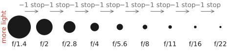
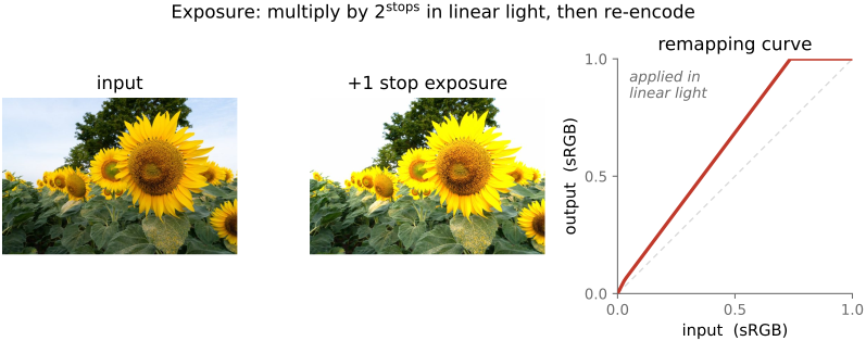
The pixel integral hands back a linear amount of light: double the aperture area or double the time and you double the number. Photographers almost never speak that way. They count light in stops, where one stop is a factor of two, because both the eye and the medium respond to ratios rather than differences (the same logarithmic story behind gamma encoding and Weber's law, Chapter 3.2, Perceptual color and trichromatic vision). A stop is the natural quantum of exposure: one doubling, one halving, one bit of light. Written on the log$_2$ scale the integral lives on, the whole messy business of exposure becomes simple addition and subtraction.
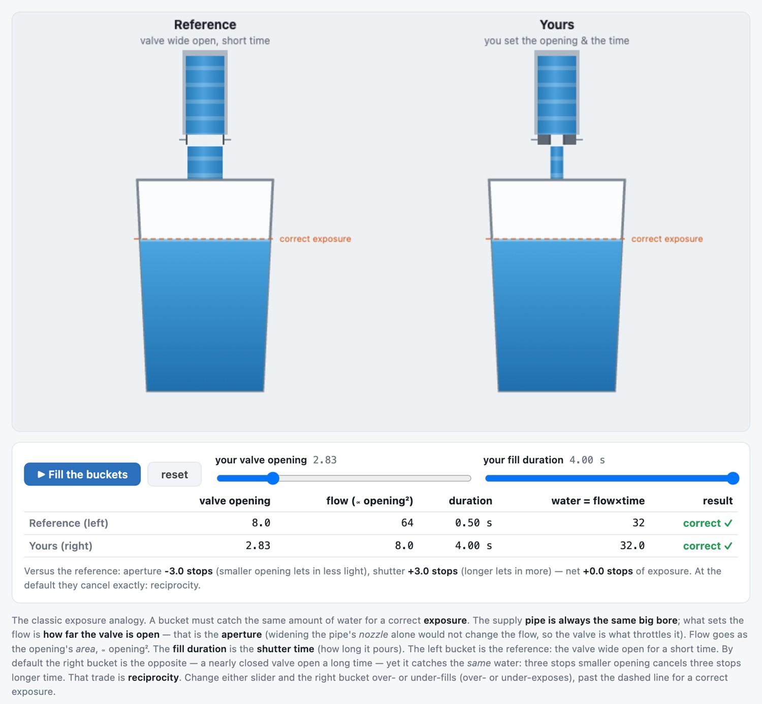
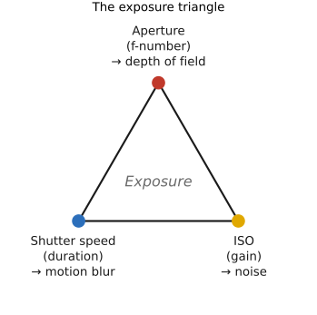
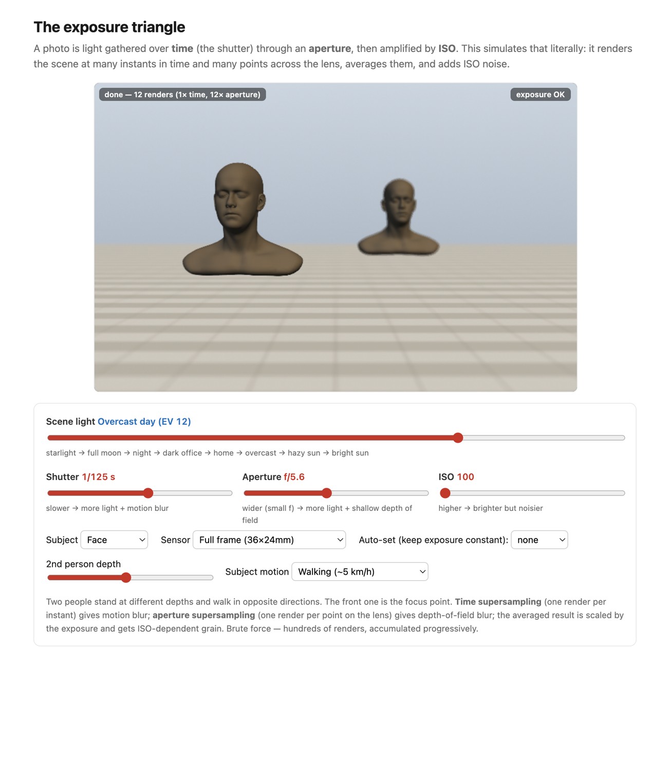
The power of the unit is that it is the same unit on every axis of the integral. One stop of aperture (a $\sqrt2$ step in the f-number, since light goes as $1/N^2$, Chapter 2.3, Lens image formation), one stop of shutter (a factor of two in time $t$), and one stop of ISO (a factor of two in gain) all change the brightness by the identical factor of two, so they can compensate one another in output brightness over an unclipped, approximately linear range. They do not preserve motion blur, depth of field, photon count or read-noise behavior. That commensurability is exactly what lets the three trade against one another, the exposure triangle: give back a stop of light on one leg, take it up on another, and the intended output brightness can remain unchanged. Many different aperture-shutter-ISO combinations therefore land on the same brightness, a redundancy photographers call equivalent exposures and rely on constantly (the faucet-and-bucket reciprocity of Chapter 5.2, Exposure and capture timing).
To name a whole family of equivalent settings with a single number, photography uses the exposure value (EV):
$$ \mathrm{EV} = \log_2\!\frac{N^2}{t}, $$
the base-2 logarithm of squared f-number divided by exposure duration expressed in seconds. EV describes aperture and shutter settings; relating it to scene luminance also requires ISO and meter calibration. One EV is one stop. Every $(N, t)$ pair on the same EV describes the same exposure, so a single EV names an entire diagonal of the aperture-shutter grid:
EV 13 (ISO 100)
$f/2.8$
$f/4$
$f/5.6$
$f/8$
$f/11$
$f/16$
shutter
1/1000
1/500
1/250
1/125
1/60
1/30
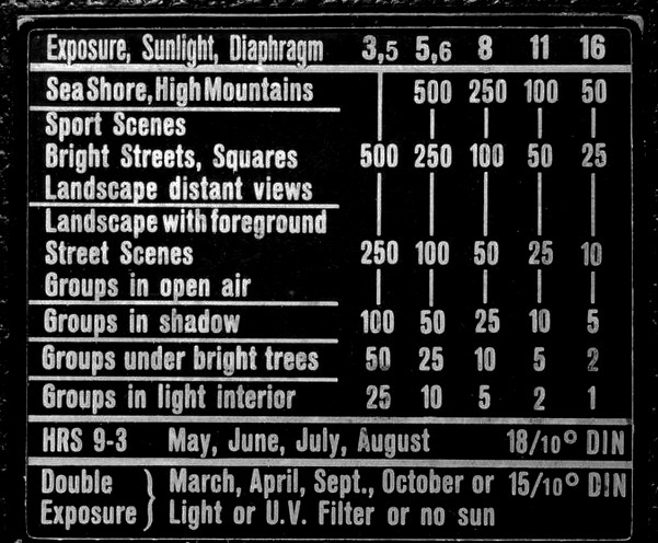
Read across: each stop you close the aperture is paid back by one stop of slower shutter, and the exposure never moves. Because EV folds the settings into one number, it doubles as a measure of scene light. At ISO 100 the same EV names how bright the scene is (sometimes called the light value): a meter's reading, $L = K N^2/(t S)$, is EV in disguise, and the old sunny 16 rule ("bright sun is $f/16$ at 1/ISO") is nothing but a printed EV chart, one EV per lighting condition.
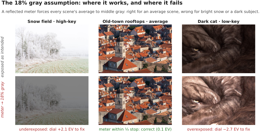
Once you have the unit, it turns up everywhere, which is the real reason to learn it. Meters report in EV, and every metered scene is placed on the EV ladder relative to mid-gray. Exposure compensation is dialed in EV ($+1$ EV to keep a snowfield white, $-1$ for a black cat), a direct nudge along the ladder. Auto-bracketing shoots frames at, say, $-2, 0, +2$ EV to merge into one high-dynamic-range image (HDR merging). A scene's dynamic range, a sensor's, a display's, are all quoted in stops (the ratio of brightest to darkest, in powers of two). Neutral-density filters are sold in stops (an ND8 is three stops), a lens's speed is "one stop faster," flash and studio lights meter in stops, and the noise story is a stop story too: because shot noise is set by photon count, every stop less light collected costs half the photons and a predictable step of signal-to-noise ratio (Chapter 2.8, Noise, signal-to-noise ratio and dynamic range). Stops and EV are the shared logarithmic language in which exposure, metering, dynamic range, filtration, and noise are all spoken; the full exposure and metering practice built on them is Chapter 5.2, Exposure and capture timing.
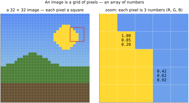
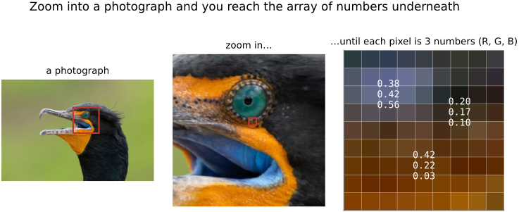
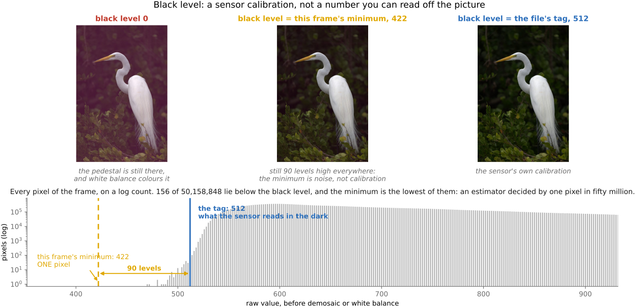
A digital sensor is a two-dimensional array of photosites, one per pixel. Each photosite is a small potential well that counts photons: arriving light frees electrons, the well accumulates that charge, and at the end of the exposure the charge is converted to a voltage and then, by an analog-to-digital converter (ADC), to a number. Because the well literally counts arrivals, the number it reports is, to good approximation, linear in the amount of light that fell on it. That linearity is not a minor technical detail: it is what lets us treat a raw image as a calibrated radiometric measurement, and it is the foundation that makes HDR merging, deblurring, and depth estimation meaningful later in the book.
💡 Big lesson (L2.35) — sensors convert photons to electrons linearly
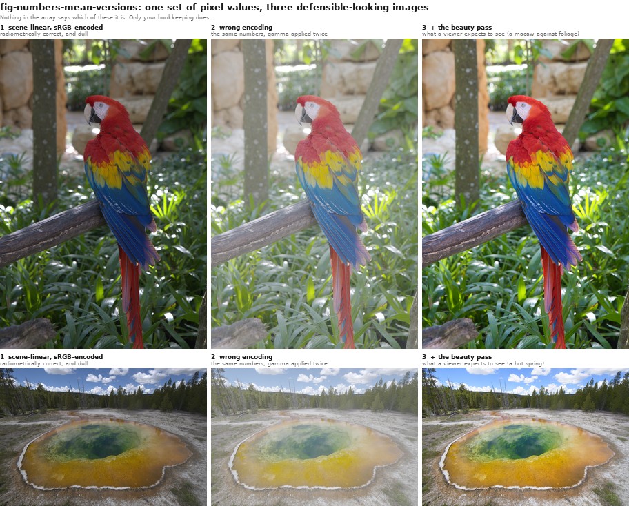
A photosite is at heart a photon counter: each absorbed photon frees a charge carrier, an electron or equivalently a hole (a missing electron), and the well accumulates them in direct proportion to the light that arrives. So the raw signal is linear in scene radiance, before any gamma or tone curve. This linearity is not a detail; it is what makes raw arithmetic trustworthy: HDR merging adds exposures, white balance is a per-channel multiply, flat-field correction is a divide, and all three are valid only because the numbers are proportional to light. Display encoding (gamma) deliberately hides this linearity for the eye, so computation should undo it and work in linear light.
Two revolutions are often conflated. The first was electronic imaging: turning light into an analog electrical signal (the era of the CCD and analog video). The second, the one computational photography lives on, was digital: putting an ADC in the path so the signal becomes numbers we can compute on. A sensor that captures light electronically but never digitizes it is a television camera, not a computer's eye.
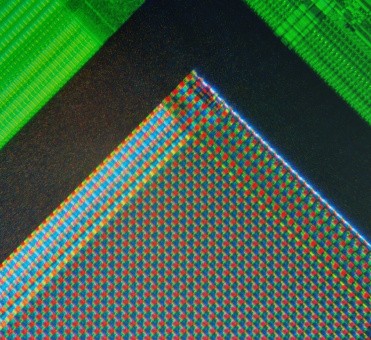
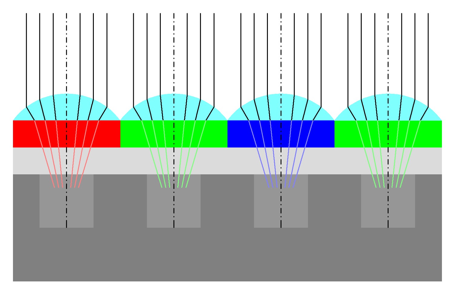
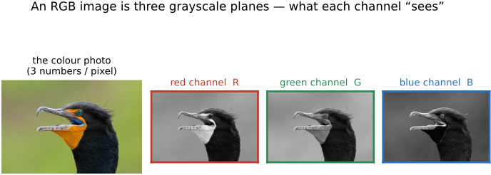
Above each photosite sits a microlens that funnels light onto the light-sensitive area, necessary because wiring occupies part of each pixel, so the fill factor is less than 100%. Under the microlens sits a color filter: a bare photosite is colorblind (it only counts photons), so a mosaic of color filters, most commonly the Bayer pattern, is laid over the grid and full color is reconstructed later by demosaicking. That is only the briefest mention here; how a colorblind sensor is made to see color, and the several ways to multiplex the measurement, is the subject of its own chapter in the next part, Chapter 4.6, Sensing color: multiplexing strategies (§4.2). Finally, the map from scene radiance to the rendered pixel value is the camera response curve: raw is roughly linear, while a JPEG has a non-linear curve (gamma plus a tone curve) baked in: recovering that curve is exactly the problem HDR has to solve.
Figure 2.7.2(reproduced). A sensor surface under the microscope. The regular grid of photosites is overlaid with the Bayer color-filter mosaic: twice as many green filters as red or blue, because the eye resolves luminance (carried mostly by green) more finely than color. Each site is one pixel's light-collecting well; full color at every pixel is reconstructed later by demosaicking.Figure 2.7.3(reproduced). A photosite in cross-section. Light enters through a microlens that gathers it onto the photosite's active area (wiring leaves the fill factor below 100%), passes a color filter (one of the Bayer mosaic's red, green, or blue), and reaches the photodiode, where it frees electrons that accumulate as charge. The charge becomes a voltage and then a digital number. Counting photons is what makes capture linear in light.
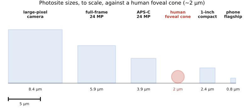
How big is a photosite, really? Pixel sizes span more than a factor of ten across cameras, and the range maps directly onto the sensor-size story below. A flagship phone crams its pixels down to about $0.7$–$1.0\,\mu\text{m}$; a 1-inch compact sits near $2.4\,\mu\text{m}$; APS-C runs $3.5$–$4\,\mu\text{m}$; a full-frame sensor is $4$–$6\,\mu\text{m}$; and the largest-pixel cameras (low-resolution full-frame bodies, astronomy and scientific sensors) reach $8\,\mu\text{m}$ and beyond. The telling comparison is biological: a foveal cone is about $2\,\mu\text{m}$ across (Chapter 3.2, Perceptual color and trichromatic vision), so a big camera pixel is several cones wide, while a modern phone pixel has shrunk below the size of a single cone (Figure 2.7.4). Size matters here because a larger collecting area receives more photons at equal irradiance and exposure, increasing shot-noise standard deviation but reducing noise relative to signal, which is the whole reason larger sensors look cleaner (→ The impact of sensor size, below). The phone's tiny wells force it to make up the deficit computationally, with burst capture and denoising rather than glass and silicon.
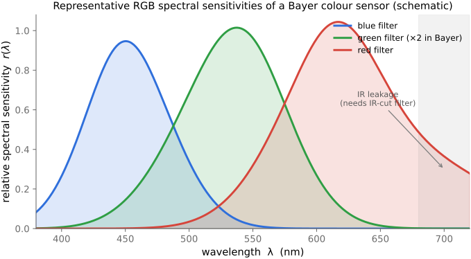
Figure 2.7.4(reproduced). Photosite sizes, to scale, against a human cone. Drawn at a common micrometer scale: a large-pixel camera (~8.4 µm), a full-frame pixel (~5.9 µm), an APS-C pixel (~3.9 µm), a human foveal cone (~2 µm, the biological yardstick), a 1-inch compact pixel (~2.4 µm), and a flagship-phone pixel (~0.8 µm). A big camera pixel spans several cones; a modern phone pixel is smaller than one cone, which is why phones must recover image quality computationally rather than optically.Figure 2.7.5(reproduced). Representative RGB spectral sensitivities of a digital color sensor. Each curve is the probability that a photon of a given wavelength, passing the red, green, or blue Bayer filter, is counted by the photosite beneath, the $r(\lambda)$ of the pixel integral. Note the broad, heavily overlapping passbands (nothing like three clean spikes), the doubled-up green sitting where the eye is most sensitive, and the long-wavelength leakage that forces an infrared-cut filter in front of the sensor. Because each channel is one number, an integral of the spectrum against its curve, very different spectra can map to the same RGB triple (metamerism, taken up with color in part 3, Chapter 3.2, Perceptual color and trichromatic vision). Curves are schematic, drawn to typical silicon-plus-Bayer shapes rather than one measured device.
Look from a distant building to a book in your hand. The eye changes focus while directing its highest-resolution region toward the words. Its optics obey the same refraction laws as a camera, but its sampling and processing differ substantially (Part 2, Fundamentals).
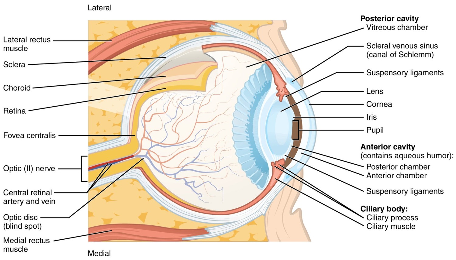
Light entering the eye passes through the cornea and the lens, the eye's two refracting elements, the same Snell's-law optics as a camera lens (the cornea does most of the bending; the lens fine-tunes focus by changing shape, accommodation). The pupil, the iris's adjustable opening, is the eye's aperture. The image lands on the retina, a thin sheet of neural tissue lining the back of the eyeball (Figure 3.1.1).
Figure 3.1.1(reproduced). Cross-section of the human eye. Light is refracted by the cornea and the lens, passes through the adjustable pupil (the aperture), and forms an inverted image on the retina at the back. The fovea is the small central pit of highest acuity; the optic nerve leaves at the blind spot.
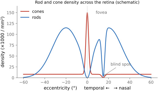
Rods and cones supply most of the signals used for image-forming vision. Rods support vision at low light levels; because they share one spectral sensitivity, rods alone cannot distinguish wavelength from intensity. Cones support daylight color vision through three receptor classes. At intermediate levels, rods and cones both contribute. Their distribution is nonuniform: cones are densest near the center of gaze, while the central foveola lacks rods (Figure 3.1.2). Looking slightly away from a faint star can therefore make it easier to detect.
Foveal cones are only a few micrometers across, with spacing near $2.5\,\mu\text{m}$ in a dense central mosaic; sizes and spacing vary across observers and retinal position. Away from the fovea the cones grow to several micrometers and thin out, while rods, about $1$ to $2\,\mu\text{m}$ across, fill the spaces between them; in Curcio and colleagues' measurements, cone density peaks near 200,000 per square millimeter at the foveal center and rod density near 150,000 per square millimeter about twenty degrees out Curcio et al. 1990. Dense sampling supports fine detail, but does not alone determine acuity. Optical blur, neural pooling, contrast, and illumination also matter. A camera photosite and a cone of similar size need not have similar sensitivity or angular resolution.
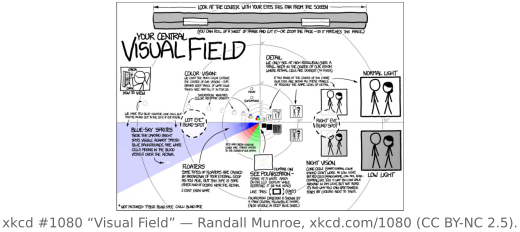
Figure 3.1.2(reproduced). *Density of rods and cones across the retina. Cones peak sharply at the fovea (the center of gaze); rods dominate the periphery and vanish at the fovea. Where the optic nerve leaves the retina, there are no photoreceptors. This produces a blind spot roughly fifteen degrees toward the temporal side of the visual field in each eye. The other eye normally supplies information from that direction. With one eye covered, a small target can still disappear into its surroundings because perception fills in the missing region (Figure 3.1.4). Filling-in depends on the stimulus; it is not a detailed measurement of the hidden object.Figure 3.1.3(reproduced). xkcd #1080 "Visual Field," Randall Munroe, xkcd.com/1080 (CC BY-NC 2.5).
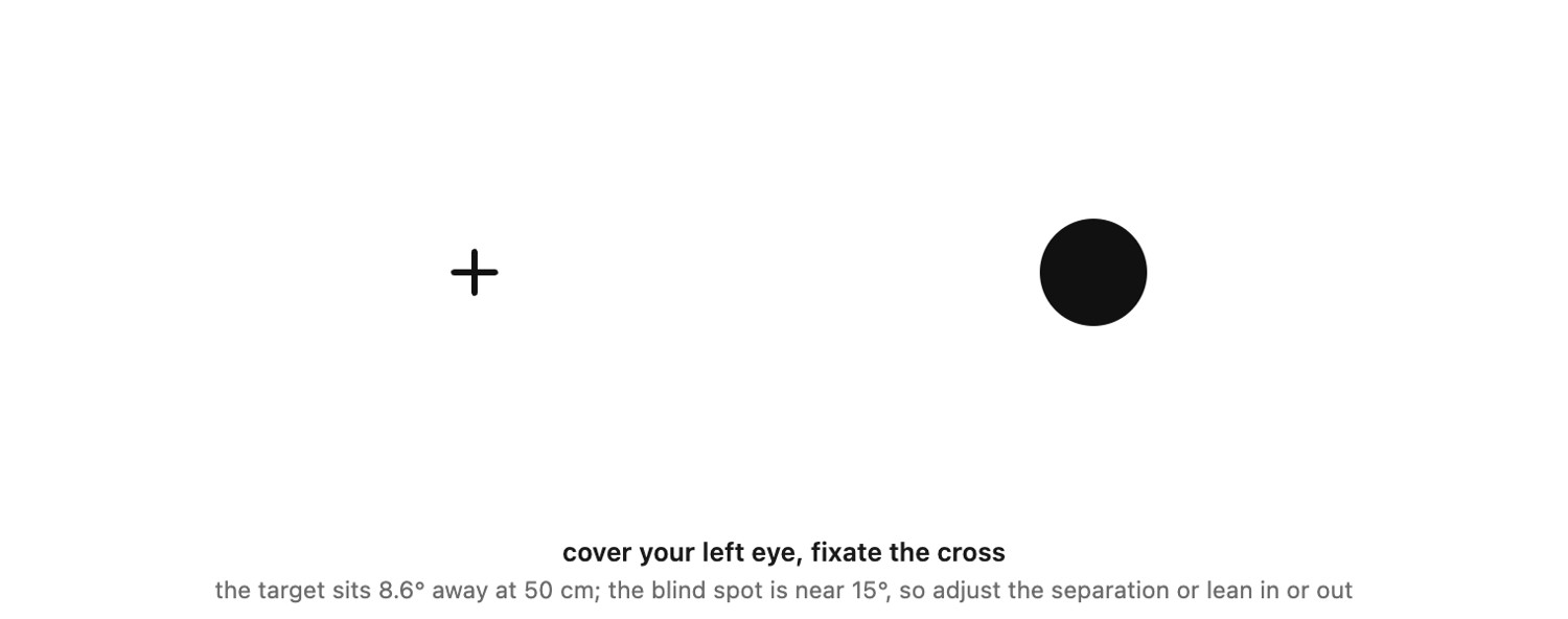
The gap at the optic disc is worth more than a label, because it is the first and cleanest evidence that what you see is constructed. Each eye has a patch of its visual field about five degrees across, some fifteen degrees to the ear side of where you are looking, that delivers nothing at all, and you have never once noticed a hole there. Two things hide it. The other eye covers that part of the field, so closing one is enough to remove the first explanation. What remains is the second and the interesting one: the missing region is filled in with whatever surrounds it, so a line broken exactly there is seen as continuous and a textured field closes over the gap. Nothing in the retina reports the fill; it is manufactured, and it is indistinguishable from the real thing (Figure 3.1.4).
Figure 3.1.4(reproduced). The blind spot, and the filling in (interactive). Cover one eye, fixate the cross, and move toward or away from the screen until the target on the other side of it disappears (with the right eye open, the target sits to the right of the cross, since the blind spot lies on the temporal side of fixation); the figure converts the on-screen separation into degrees once you tell it your viewing distance and your screen's pixels per centimeter, since the eye works in angle and the page cannot know either number. Try the three targets. A disc on a plain field vanishes, which is the hole. A break in a line vanishes and the line is seen running straight through, which is the fill. A hole in a texture closes over with the texture, which is filling-in of texture. The vanishing point sits near fifteen degrees; if it does not, adjust the separation rather than your seat.
S cones are sparse and absent from a small region at the very center of the fovea. Short-wavelength detail also suffers from the eye's chromatic aberration. Fine luminance detail is carried mainly by combined L- and M-cone signals, while purely chromatic variations have lower spatial resolution. This does not make a green channel identical to luminance, or imply that blue detail is universally sharp through filling-in. The relative importance of luminance detail helps motivate the extra green samples in the Bayer pattern (Chapter 4.6, Sensing color: multiplexing strategies).
The retina processes signals before sending them along the optic nerve. Photoreceptors connect through intermediate neurons to ganglion cells. Many ganglion cells compare a central region with its surround, making them sensitive to local contrast; others have different spatial, temporal, or chromatic selectivity. Signals then reach several brain regions, including the lateral geniculate nucleus and visual cortex. A camera-to-retina analogy is useful for the optics, but retinal output is already a collection of processed signals.
Focus errors provide another connection to camera optics. In a simplified eye, myopia places the image of a distant point in front of the retina; hyperopia places it behind the retina when accommodation is relaxed. Astigmatism gives different focusing power along different orientations. Presbyopia reduces the range over which accommodation can adjust focus with age. These are different optical problems, not one generic blur.
Lens power is expressed in diopters:
$$P=\frac{1}{f},$$
where $f$ is the signed focal length in meters. A converging lens with focal length $0.5$ m has power $+2$ diopters; a diverging lens of $-0.5$ m has power $-2$ diopters. This describes the lens, not a complete eye prescription: cylinder power and orientation also matter for astigmatism.
An autorefractor estimates refractive error from light returned by the eye; subjective comparison with trial lenses refines the result. A Shack–Hartmann sensor measures the slopes of the outgoing wavefront using a lenslet array, allowing more detailed aberration estimates. The shared imaging idea is to infer optical properties from the recorded light. Part 22, Compound lenses, and aberration correction develops wavefront measurement.
A white shirt can remain recognizably white under daylight or a warm lamp despite a change in the spectrum reaching the eye. Color constancy describes this approximate stability of surface-color judgments. It does not imply recovery of the surface's full reflectance spectrum. Illuminant estimation, adaptation, and spatial context all contribute.
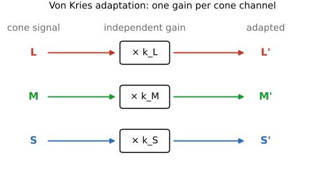
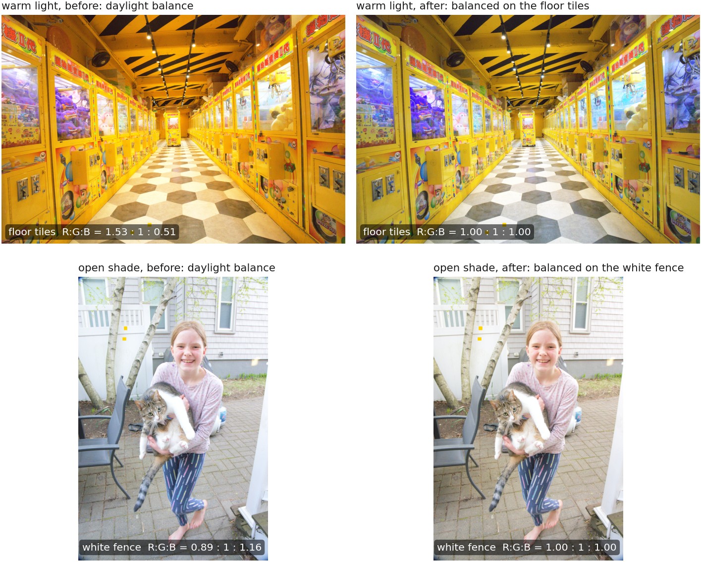
Von Kries adaptation models an independent gain on each cone class Von Kries (Figure 3.3.16). Gains chosen to map an adapting white to a reference white give a useful approximation, not exact illuminant removal for every surface. Chapter 4.2, White balance and white point develops the corresponding transform and its limits.
Figure 3.3.16(reproduced). Von Kries cone-gain adaptation. The same surface viewed under two different illuminants produces different cone responses; an independent multiplicative gain on each of the L, M, and S channels rescales them so the surface reads as the same color. This per-channel gain is the perceptual blueprint for camera white balance.
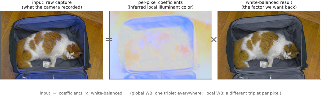
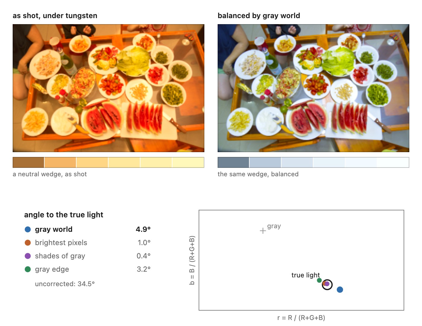
Camera white balance estimates gains or a more general transform to render the scene for the intended output. Gray-world, bright-pixel, and learned methods use different evidence. These engineering estimators need not duplicate the visual system's computation Freeman & Brainard (Bayesian color constancy).
In low light, weak cone signals and increased rod contributions reduce color discrimination. A camera that accumulates a burst may record color that was difficult to see during capture. Night Sight uses learned white balance as part of a pipeline demonstrated down to 0.3 lux Liba et al. 2019. That illuminance is a capture condition, not a universal threshold below which no person has useful color information. The desired rendering may also preserve some warmth or darkness rather than fully neutralizing the scene.
💡 Big lesson (L3.12) — the eye discounts the color of the illuminant
Chromatic adaptation and scene interpretation help stabilize surface color across illuminants. Per-channel cone gains are a useful approximation. Camera white balance makes a related rendering choice for the output conditions, with accuracy limited by the measurements and estimated illuminant.
Failure of color constancy when viewing photographs⧉
A photograph supplies cues about a depicted scene while also being an object viewed under different conditions. The display white, room lighting, image content, viewing angle, and adaptation state can all influence its appearance. A tungsten-lit scene on a daylight-balanced display may therefore look more orange than the scene did during capture. White balance helps choose the intended relationship between capture and viewing conditions; it need not remove every visible trace of the illuminant.
Experiments show that constancy depends on scene cues and on what observers are asked to match Kraft & Brainard 1999Arend & Reeves 1986Brainard et al. 2006 (Bayesian human constancy). Displayed images can support substantial constancy when they supply useful cues. A photograph does not switch that ability off. Color-appearance models describe effects of specified viewing conditions, but should not be confused with ICC rendering intents or a complete account of scene interpretation Fairchild, Color Appearance Models.
There is also a measurement limit. Two surface spectra can produce the same camera channels under one illuminant and different responses under another. No deterministic mapping of that single triple can separate the surfaces. White balance cannot reconstruct wavelengths that the illumination did not supply. This matters with narrowband sources and is distinct from a viewer's incomplete adaptation (Chapter 3.2, Perceptual color and trichromatic vision).
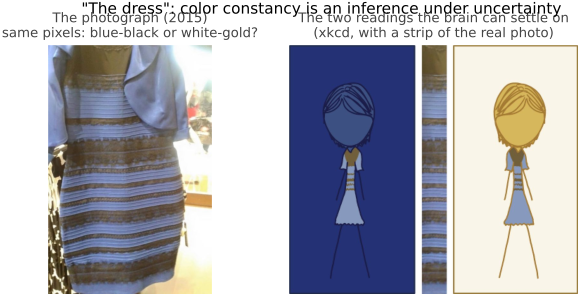
The 2015 photograph of “the dress” demonstrates that viewers can interpret the same displayed image differently Lafer-Sousa et al. 2015 (Figure 3.3.17). Assumptions about illumination contribute to the blue-black and white-gold reports. The effect supports the role of inference under ambiguous conditions; it does not prove that two simple illuminant choices fully explain every observer's response.
💡 Big lesson (L3.13) — capture and viewing conditions both affect color appearance
A photograph is viewed under conditions different from those at capture. Its appearance depends on the display or print, the surround, adaptation, and cues within the picture. White balance and rendering should target those conditions and the photographer's intent; viewers do not automatically undo the captured illuminant.
A print has two illumination contexts. Light in the room falls on the paper; within the image, shadows and highlights depict light that fell on the original scene. The viewer can recognize both, but they need not support the same adapting white. This is the dual character of picture perception discussed by Mausfeld Mausfeld 2003 (dual code). It explains why simply reproducing the captured color coordinates need not reproduce the appearance experienced by the photographer.
For example, consider a white wall photographed under a warm lamp and shown on a display in a daylight-lit room. The camera measured the warm spectrum reflected by the wall. Displaying that cast unchanged can make the wall appear more orange than it did to someone adapted to the original room. White balance supplies a rendering decision about that difference. Neutralizing every surface is not compulsory: the photographer may want the warmth of the lamp to remain. The distinction is between a measurement of the light that arrived and a choice about how the scene should look under new viewing conditions.
The inference is difficult because the camera did not separately measure illumination and reflectance. A correction toward a reference illuminant uses assumptions about the source and the surfaces. If the source supplied almost no energy in some wavelength range, the photograph contains little evidence about reflectance there. A plausible correction cannot manufacture that evidence. This connects the perceptual motivation for white balance to the spectral measurement limits developed in the color part.
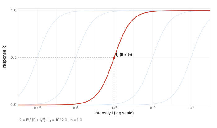
Walk into a dark cinema and details gradually become visible. The visual system changes sensitivity as the prevailing light changes. A useful model of a saturating response is the normalized Naka–Rushton curve Naka & Rushton 1966,
$$R=\frac{I^n}{I^n+I_0^n}.$$
At intensity $I=I_0$, the response is one half. Changing $I_0$ moves the operating range; $n>0$ controls the slope. This family can describe measured responses, but one curve and a moving average do not specify all of light adaptation. The curve is sigmoid when plotted against log intensity; for $n=1$ on linear axes it is a saturating hyperbola.
Figure 3.3.1 lets you change the operating point and compare axis scales.
Figure 3.3.1(reproduced). Light adaptation as a sliding response curve. The neural response $R = I^n/(I^n + I_0^n)$ is an S-shape whose half-saturation point $I_0$ marks where the response is half-maximal; adaptation slides $I_0$ to track the prevailing light, so the eye's limited response range is always spent where the light actually is. Drag the adaptation-level slider (log scale) and the whole curve translates along the intensity axis; the faint curves are the same shape at other adaptation levels. On a log-intensity axis the slide is a pure horizontal shift; switch to log-log or linear axes, or raise n to steepen the transition.
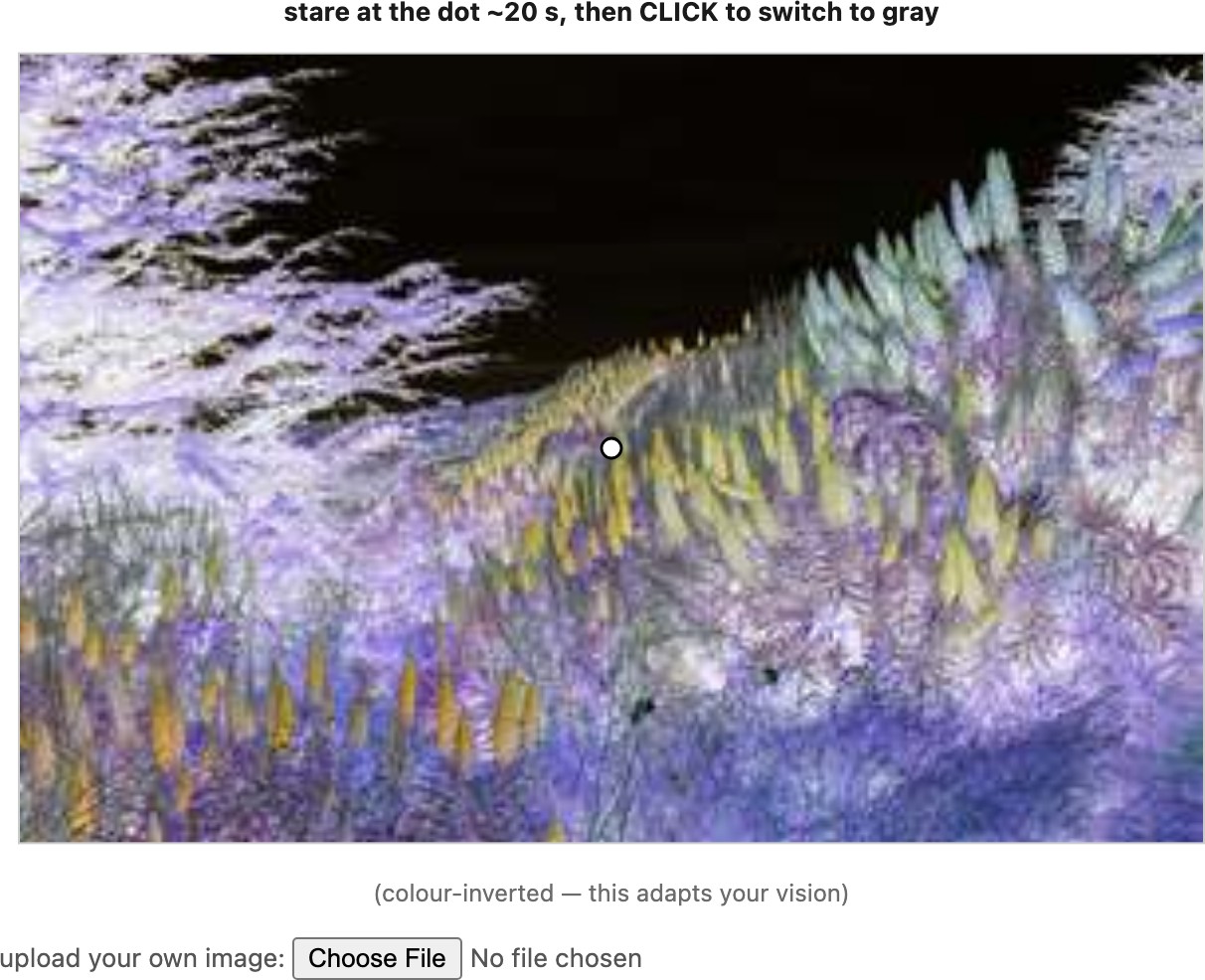
Neural gain control, photopigment bleaching and regeneration, and pupil changes contribute on different timescales. A pupil diameter change from 2 to 7 mm changes area by $(7/2)^2\approx12$, much less than the full range over which vision operates. Full dark adaptation can take tens of minutes. Local adaptation also contributes to afterimages. In the Spanish-Castle demonstration, an adapting color image is followed by a grayscale version that briefly appears colored (Figure 3.3.3); the effect is not an illusion of motion.
💡 Big lesson (L3.7) — the eye's dynamic range is enormous over time and modest at any instant
Distinguish sensitivity across adaptation states from the range visible in one scene under specified conditions. Local adaptation, glare, spatial structure, and the task all affect that range. A single stop count is insufficient to compare an eye, camera, and display.
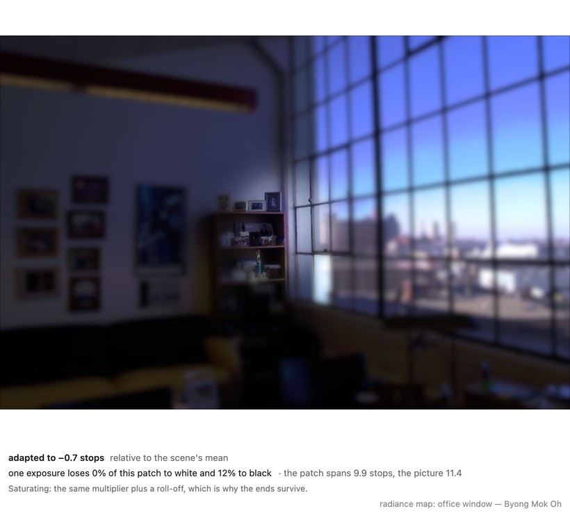
Figure 3.3.2(reproduced). One gain per fixation (interactive). A real radiance map, ten stops or more from its darkest corner to its brightest, far more than a display or any single instant of vision can show. Move the pointer. Inside the soft aperture the scene is rendered for the light at that spot; outside it, the same scene gets the one linear exposure a camera has to choose, and you can set it the two ways a photographer can: for the average, which places the mid-tones and burns the highlights out, or for the highlights, which keeps them and drops everything else into the dark. On the office the two are about six stops apart, and neither one shows you the room and the city outside the window at once, which is the whole trouble; on the design-center interior they are eleven stops apart and the gap is starker still. Nothing about the scene changes as you move, only the gain, and that is enough to make every part of it readable in turn: the readout says how much of what is under the aperture the single exposure loses at each end, to white and to black. Saturating is the previous figure's Naka-Rushton curve with its half-saturation slid to the local level, so the ends roll off; gain only is a pure multiplier, which rescales but compresses nothing, so whatever range the aperture itself contains still clips. Adaptation is lagged rather than instant, in the log domain because the mechanism is multiplicative; set the time constant to zero and the effect is uncanny, because instant adaptation is not what having eyes is like. The readout also shows where a single gain is not enough: park the aperture on a bright doorway edge and one fixation spans nearly the whole picture's range, which is what local tone mapping later in the book exists to handle. Eight radiance maps to choose from, each at its own proportions. A cartoon in five specific ways: the eye pools its adapting level over a far larger and softer region than this aperture and with a strong whole-field component, so the sharp boundary is an artifact; only the fast neural gain is modeled, not the photopigment bleaching that takes minutes nor the pupil; a real surround still contributes to the pool rather than being ignored; the eye never holds still, so you never see a scene at one gain the way a frozen aperture suggests; and the peripheral blur is a separate simplification standing for the fall-off of acuity away from the fovea, a different mechanism from adaptation and nothing like a uniform blur, present so you can see where you are looking and switchable off, and computed in linear light, which is why a blown highlight spreads into what is beside it. Radiance units in a Radiance file are arbitrary unless calibrated, so levels are quoted in stops relative to each scene's own geometric mean, not in cd/m². Radiance maps by Paul Debevec and Byong Mok Oh.Figure 3.3.3(reproduced). The Spanish-Castle illusion, a demonstration of color adaptation. Fixate the center dot on the color-inverted picture for about 20 seconds (hold your gaze steady); this bleaches your opponent channels locally. Then click to switch the same picture to grayscale and, for a few seconds, your rebounding channels paint it back in near-natural color before the afterimage fades. Pick one of our images or upload your own; it is processed entirely in your browser.
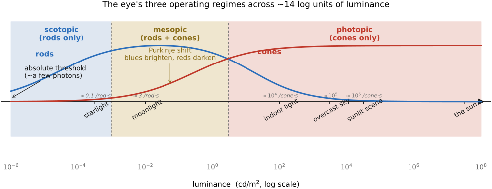
Vision is often described in three regimes. Photopic vision is cone-dominated and supports detailed color vision. Scotopic vision is rod-dominated and lacks ordinary trichromatic color discrimination. Mesopic vision combines rod and cone signals. The transitions depend on adaptation, spectrum, retinal position, and stimulus, so they are not universal luminance cutoffs.
As illumination falls, relative spectral sensitivity shifts toward shorter wavelengths, the Purkinje shiftPurkyně 1825 (Purkinje shift). A red flower can become relatively darker than nearby blue-green foliage. This is a change in relative sensitivity, not a statement that all dim scenes look blue. Luminance (cd/m²) describes light from a surface in a viewing direction; illuminance (lux) describes light arriving at a surface. A scene's lux value alone does not determine the observer's adaptation state.
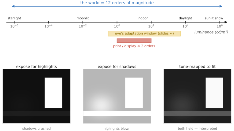
Figure 3.3.4(reproduced). The three operating regimes on a log-luminance ($\text{cd/m}^2$) axis: scotopic (rods only), mesopic (rods and cones), and photopic (cones only), with the rod and cone activity curves, the absolute threshold of vision, the Purkinje shift in the mesopic band, and real-world landmarks placed along the axis: starlight → moonlight → indoor light → overcast sky → sunlight → the sun. Each landmark also carries the photons caught per receptor per second (photoisomerizations): from about $0.1$ per rod per second under starlight (one photon every ten seconds or so) up to ${\sim}10^{6}$ per cone per second in a sunlit scene. These counts fold in the pupil (iris), which narrows from about $7\,$mm in the dark to about $2\,$mm in bright light, and switch from per-rod (scotopic) to per-cone (photopic) as the receptors hand over.
Retinal illuminance is often summarized in trolands: luminance in cd/m² multiplied by pupil area in mm²,
$$T=L_v A_p.$$
For example, a 100 cd/m² patch viewed through a 3 mm diameter pupil gives about $100\pi(1.5)^2\approx707$ trolands. This is a photometric convention, not a universal conversion to photons. For order of magnitude only, Rodieck's estimates put a rod under starlight at roughly one photoisomerization every several seconds, and a cone in a sunlit scene at around a million per second Rodieck, The First Steps in Seeing, a span the pupil, bleaching and neural gain together have to accommodate. Predicting photoisomerizations additionally requires the spectrum, ocular transmission, receptor sensitivity and collecting area, and integration time. A photon absorbed by a visual pigment can isomerize the molecule and initiate a graded receptor response; it does not necessarily cause a perceptible event.
At very low light levels, photon statistics and neural noise limit detection. Hecht, Shlaer, and Pirenne inferred that a detectable flash could produce only a few photoisomerizations distributed across many rods Hecht, Shlaer & Pirenne 1942. Recordings subsequently established that individual rods can respond to single photons Rieke & Baylor 1998. That cellular response must be distinguished from conscious detection. Tinsley and colleagues reported slightly above-chance detection of single photons incident on the cornea Tinsley et al. 2016 (humans detect a single photon), but later retinal and psychophysical work challenged the interpretation of that result (2024 study). These findings do not make the eye a reliable photon counter. Chapter 2.8, Noise, signal-to-noise ratio and dynamic range explains the corresponding photon-counting limits in cameras.
The range over which we can function after adapting is much greater than the range we can distinguish at one operating point. A bright scene and a dark cinema do not both fit into one unchanged receptor response. Adaptation moves that response so its useful slope falls near the current stimulus levels. This is why a claim about the eye's total dynamic range does not specify how many stops a display must reproduce simultaneously. HDR capture and tone mapping must account for the scene, the display, and the observer's adaptation separately.
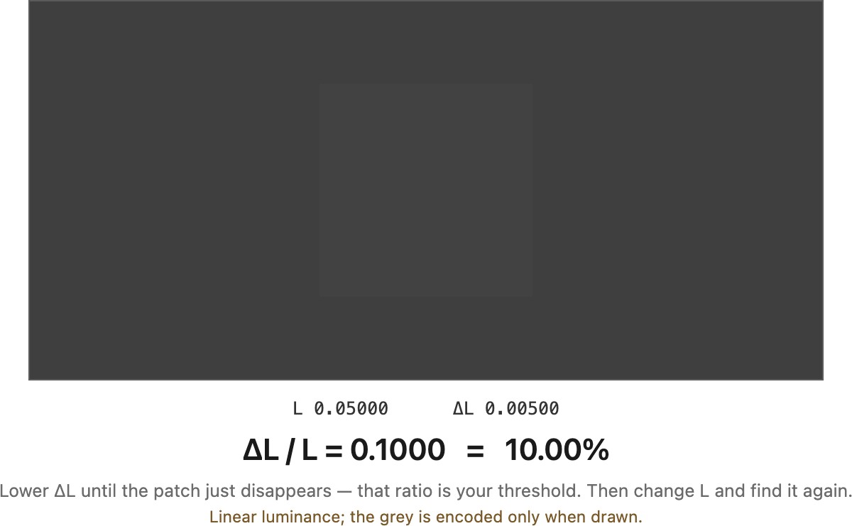
If vision reads ratios, its natural unit is contrast, and the oldest quantitative statement of that is Weber's law (Weber 1834 (Weber's law)): the just-noticeable increment in intensity is a roughly constant fraction of the background, $\Delta I / I \approx \text{const}$. The smallest brightness change you can detect grows in proportion to the brightness already there. A candle added to one candle is obvious; the same candle added to a hundred is nothing.
Figure 3.3.6(reproduced). Measure your own Weber fraction (interactive). A patch of increment $\Delta L$ on a background $L$. Lower $\Delta L$ until the patch just disappears: the ratio $\Delta L/L$ you land on is your threshold, and it is the quantity Weber's law is about — the smallest detectable increment is a roughly constant fraction of the background. Now change $L$ by a factor of ten and find the threshold again: $\Delta L$ will have moved by roughly the same factor while the ratio comes back to about where it was. In good conditions that ratio is a few percent; on a screen in a lit room expect worse, because light reflected off the glass adds a constant veil to patch and background alike, turning the quantity into $\Delta L/(L+L_0)$ and hurting dark backgrounds most. Two caveats: you know where the patch is, which lets you detect a smaller increment than a proper forced-choice experiment would, and Weber's law holds only over the middle of the range — near black the threshold stops falling and flattens out. Values are linear luminance; the gray is encoded only when drawn.
Weber's law is a statement about threshold. It describes the smallest increment you can just detect, and there it holds well across the middle of the photopic range, but it says nothing about how strong a large, plainly visible contrast looks. That suprathreshold regime has its own accounts, and two classical ones matter here. Fechner integrated Weber's law, treating each just-noticeable difference as one equal step of sensation, and reached a logarithmic relation between intensity and perceived magnitude, $\psi \approx k \log \phi$ Fechner 1860 (Elemente der Psychophysik). Stevens, from direct magnitude estimation, argued instead for a power law, $\psi = k\,\phi^{a}$, with an exponent that depends on the modality Stevens 1957 (power law). Which is right has been argued for a century and does not need settling here.
These models preserve different relations. A common scale leaves Weber contrast unchanged. Under Fechner's model it adds a constant to perceived magnitude, preserving differences; under Stevens's model it scales magnitude, preserving ratios. Neither implies unchanged brightness. Gamma encoding is a power law and does not turn a multiplier into an additive offset; a logarithm does.
For a small target on a uniform positive background $L_b$, use Weber contrast. For a periodic grating, use Michelson contrast:
The first measures a target's increment or decrement relative to its background. The second measures modulation relative to the midpoint of a periodic pattern's extrema. Both cancel a common positive multiplier, but they describe different stimuli. For luminances 80 and 120, Michelson contrast is 0.2; a 120 target on an 80 background has Weber contrast 0.5. Use linear luminance, not encoded pixel values.
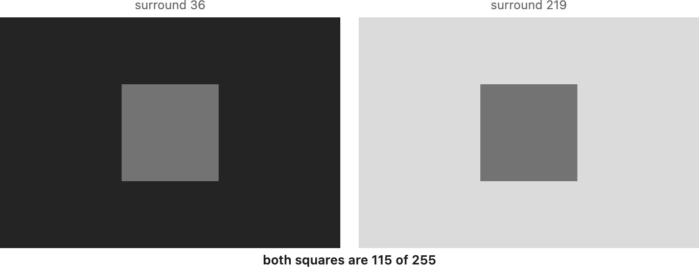
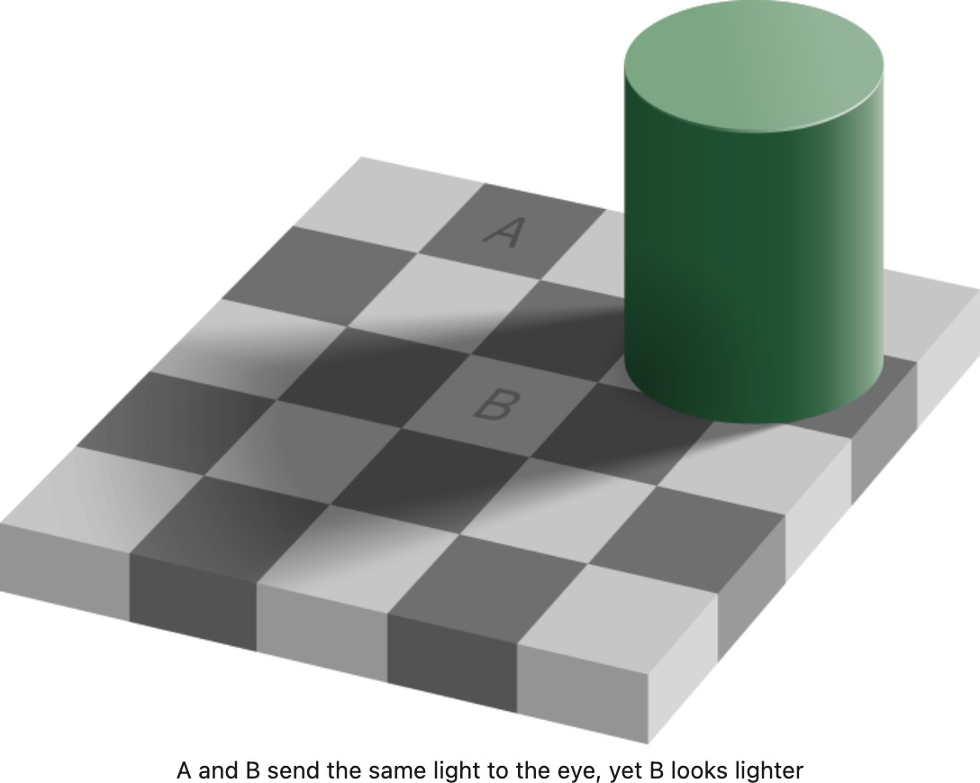
Contrast is set by context too, not by a patch in isolation. A gray patch looks lighter on a dark surround and darker on a light one, the effect called simultaneous contrast (Chevreul 1839 (simultaneous contrast)), while the Adelson checker-shadow illusion adds cues about scene geometry and illumination. Meet it in its barest form before any tone-mapping operator arrives, because every one of them is a machine for changing exactly this (Figure 3.3.7).
Figure 3.3.7(reproduced). One gray, two surrounds (interactive). The two squares are filled from the same number, printed under them; the surrounds are not. Slide the surrounds apart and the two squares separate perceptually while staying identical in the file. The bridge is the part worth doing: join them with a bar of that same gray and the difference largely collapses, because what the visual system compares is regions, and a bar that connects them makes them one region rather than two. Switch the two fields for a single slow gradient and the effect survives with no border to blame it on.
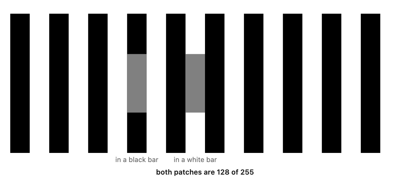
That much is compatible with a simple story: the response to a patch is divided by the light around it, so more surround means a darker-looking patch. Simple surround averaging cannot account for White’s illusion (Figure 3.3.8), which is a counterexample to simple surround division: the patch that looks lighter is the one with more white against it, which is the opposite of what dividing by the surround predicts. Perceptual grouping and junction structure contribute beyond immediate border contrast.
Figure 3.3.8(reproduced). White's illusion (interactive). Two patches of one gray on a square-wave grating, at the same height, one replacing a segment of a black bar and one a segment of a white bar. The patch in the black bar looks lighter. Ordinary simultaneous contrast predicts the reverse: lying inside a black bar means the patch's two long sides run against the white bars on either side, so it is the patch with more white against it. Turn on measure the borders and the figure counts it, at the default size 25% of one patch's outline runs against black and 75% of the other's, exactly backwards from the percept. Put the same two patches on plain black and plain white instead and the pair separates the other way, which is the control.
💡 Big lesson (L3.10) — contrast depends on a reference level
Detectable increments often scale approximately with the background in the photopic range. State which contrast definition, stimulus, and viewing conditions a measurement uses. Absolute pixel error and perceived difference answer different questions; neither replaces the other.
A white page in shadow can look lighter in surface color than sunlit coal even if the coal sends more light to the eye. Lightness is perceived surface reflectance; brightness is the perceived amount of light. Lightness constancy is approximate stability of the former as illumination changes. It is not exact recovery of physical reflectance.
In the simple product model, separating illumination and reflectance from one image is underdetermined. Vision uses context, edges, spatial organization, and prior experience. A sharp edge can be a reflectance boundary or a shadow; a smooth variation can be illumination or a surface pattern. No rule that classifies edges by sharpness alone solves the problem.
Adelson's checker-shadow illusion shows two equal pixel values that appear to belong to different surface lightnesses Adelson 2000 (Figure 3.3.9; source explanation). Shadow cues and local relationships support different interpretations of the two squares. Retinex models use spatial comparisons to estimate lightness Land & McCann 1971, and intrinsic-image methods explicitly separate reflectance and shading. These are models of the inference, not established descriptions of a single neural algorithm.
Figure 3.3.9(reproduced). Adelson's checker-shadow illusion. The square labeled A (in light) and the square labeled B (in the cylinder's shadow) have identical luminance, yet B looks far lighter, shown side by side with a proof strip connecting the two equal-gray squares. The visual system discounts the inferred shadow and reports surface lightness, not luminance.
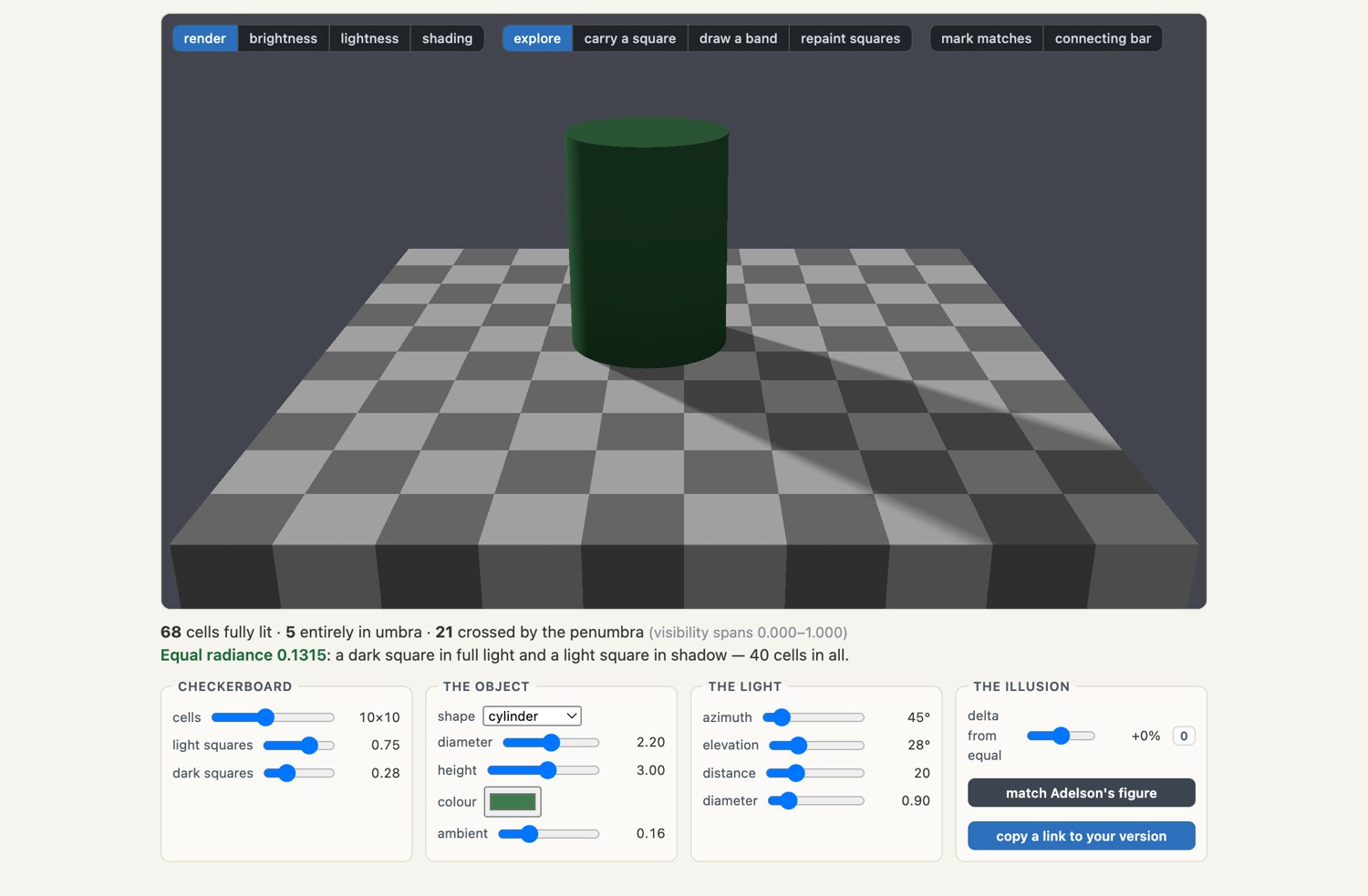
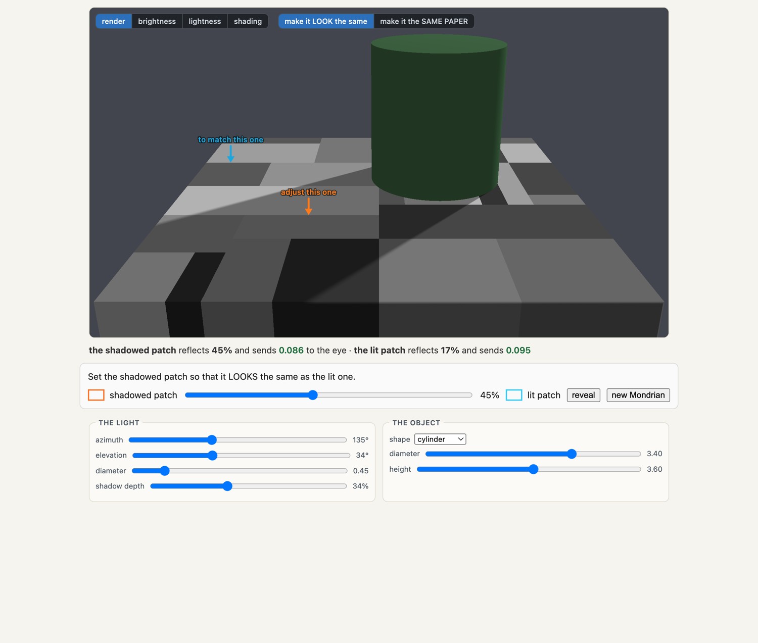
Video 1. Video: Incredible Shade Illusion! by brusspup, a physical demonstration of the checker-shadow effect: cover the surround and the two squares are plainly the same gray (YouTube).Figure 3.3.10(reproduced). The same illusion, generated rather than painted (interactive). Adelson's original is artwork: the two squares are drawn with the values that make the point. Here the scene is actually rendered — a checkerboard, an object standing on it, and a shadow computed from supersampled shadow maps cast by a light of finite diameter, which is where the penumbra comes from. The equality that carries the illusion is one deliberate choice: the umbra level is set to dark ÷ light, so a light square in shadow leaves exactly the radiance of a dark square in the open. Move delta off zero and the equality breaks, and the illusion goes with it. Two departures from physics are also deliberate: the object gets a correct per-point cosine, but the board gets the cosine at its center everywhere, and nothing gets distance falloff — a real point source would light the near edge of the board more than the far one, and that gradient would give the game away. The readout is computed from the G-buffer rather than asserted: a cell counts as fully lit only if every one of its pixels saw every light sample, and as umbra only if none did; cells the penumbra crosses are excluded, because their radiance genuinely varies across the cell. Switch between the render, the brightness it actually carries in false color, the lightness of the surface alone, and the shading alone — the decomposition the visual system has to solve. Change the board, the object (a cylinder, a chess rook, a chess pawn, or a teapot), the light and the shadow softness; drag the object to a different square, and copy a link to your version. Repaint squares hands you the board itself: click a square and it flips from light to dark or back, and the change sticks, so you can put a light square where the shadow falls and a dark one where it does not and watch the measurements follow. The pattern is not what makes the illusion, the reflectances and the shadow are. Match Adelson's figure sets the scene to his: eight squares across, the cylinder standing back and to the right, and a reflectance ratio of 3.1 to one, which is what his released image measures, since a light check reads 200 there while squares A and B both read 120, and undoing the sRGB encoding turns those into 0.578 and 0.184. The brightness scale is jet, chosen because it is not smooth: hue races through it, so two patches carrying the same radiance land on the same conspicuous color rather than on two shades of gray nobody can compare across a picture. (The chess pawn was generated with Meshy.)Figure 3.3.11(reproduced). The matching experiment, run inside a rendered scene (interactive). This is the previous figure's machinery, a real board with a real object casting a real soft shadow, carrying Arend & Reeves 1986's task instead of Adelson's demonstration. The checkerboard is replaced by a Mondrian, because a checkerboard has only two reflectances and the answer can be guessed, while a Mondrian has a dozen and offers nothing to lean on, which is exactly why Land used them (Land & McCann 1971). One rectangle lies entirely inside the umbra and one entirely in the open, and that is measured off the G-buffer rather than asserted: a rectangle qualifies only if every one of its cells saw every light sample, or none of them did. The two are pointed at by arrows that keep clear of the board and vanish while you move the slider: a box drawn around a patch is a local contrast, and it would do the judging for you. Your job is to set the reflectance of the shadowed one until it matches the lit one, under one of the two instructions Arend and Reeves showed give different answers. Make it look the same asks for equal light arriving at your eye, which needs a much paler paper in the shadow. Make it the same paper asks for equal reflectance, which sends far less light to your eye and looks darker. Then press reveal: both answers are marked on the scale beside where you landed, along with a constancy index, 1 for a paper match and 0 for a light match. Neither answer is wrong. The gap between them is the size of the discount the visual system applies to an illuminant it has inferred, and the fact that a wording change moves your setting between them is the finding. Switch to lightness to see the reflectances alone, shading for the illumination alone, and brightness for what actually reaches the eye.
loading community examples…
Figure 1.community Built a variant worth seeing: an object, a board, or a light that makes the illusion stronger or breaks it? Copy the link from the figure and share it with other readers.
The Gelb effect illustrates the importance of context Gelb 1929 (the Gelb effect). A black paper illuminated by a hidden spotlight in a dark surround can appear white. Adding a white reference can make it appear darker. The result depends on how the visible surfaces are grouped and interpreted; it does not establish perfect constancy in ordinary scenes.
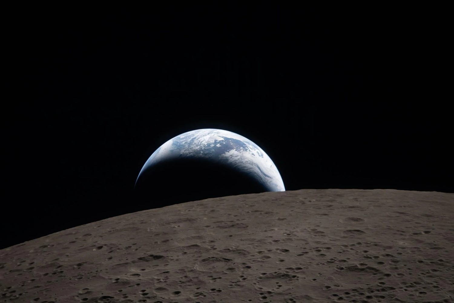
The Moon provides a familiar comparison. Its average reflectance is low, yet against a dark sky it can appear bright and nearly white. Brightness and surface lightness are different judgments: strong illumination can make a dark material bright. Images containing both Earth and Moon help compare their reflected light (Figure 3.3.13), although exposure, geometry, and rendering also affect the photograph.
Figure 3.3.13(reproduced). The moon is far darker than it looks. Here the crescent Earth rises over the cratered gray surface of the Moon, and even beside our own sunlit planet the lunar ground reads as the dark material it is: an average reflectance near $0.12$, about that of worn asphalt. On its own against a black sky the full moon still reads as bright and near-white, because nothing sits beside it to set the scale; here the bright Earth supplies exactly that missing reference. NASA.
Video 2. Video: The DSCOVR spacecraft's EPIC camera watches the fully-lit far side of the Moon cross the sunlit face of Earth, from a million miles out. Both discs are in full sunlight, yet the Moon is unmistakably the darker, grayer one, a moving demonstration that its reflectance is far below Earth's. NASA/DSCOVR EPIC imagery (YouTube).
Estimating stable surface properties helps recognize materials across lighting changes. Illumination is also useful information: it describes shadows, shape, weather, and time of day. Vision does not simply discard it, and a photographer may choose to emphasize it.
💡 Big lesson (L3.11) — surface appearance can remain stable as illumination changes
Surface-lightness and color judgments can remain relatively stable as illumination changes. This constancy is partial and uses several cues. It differs from recovering the complete reflectance spectrum, and it does not imply that brightness or the appearance of lighting stays fixed.
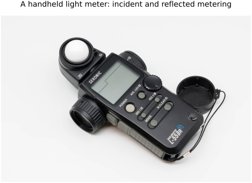
An incident-light meter or a known gray reference helps choose an exposure without mistaking a dark subject for weak illumination. Their use does not guarantee the same rendering in all conditions: orientation, lighting variation, meter calibration, and clipping still matter (Chapter 5.2, Exposure and capture timing).
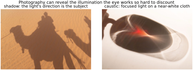
Lighting can be the subject of a photograph. A long cast shadow records the direction of sunlight; a caustic on a nearly uniform cloth records how glass redirects it (Figure 3.3.14). The print represents those variations as ink reflectance, while a display represents them as emitted light. The viewer can still interpret them as illumination in the depicted scene.
Figure 3.3.14(reproduced). Photography can reveal the illumination the eye works so hard to discount. Left: a camel ride at low sun, where the long cast shadow of camel and riders on the orange sand is the picture, so the light's direction and hour become the content. Right: a caustic thrown by a curved glass onto a nearly white cloth, a bright cusp with a red chromatic fringe; because the cloth's reflectance is close to uniform, the frame records the focused light itself. On a uniform surface the illumination pattern becomes the image, and once printed that light is turned into a fixed reflectance on the page. Photographs by Frédo Durand.
loading community examples…
Figure 2.community Upload your own photo that makes lighting and shadows the subject to share with other readers.
A photographer can deliberately make illumination the subject. On a nearly uniform white cloth, a glass casts a caustic whose structure comes mainly from the redirected light rather than a change of material. A low sun can make a person's shadow a stronger graphic shape than the person. Printing the photograph fixes those variations as different ink reflectances, so the pattern can be examined under new lighting long after the original caustic or shadow has disappeared. This does not prevent the viewer from recognizing depicted illumination; it separates the light on the print from the light represented by the print (Figure 3.3.14).
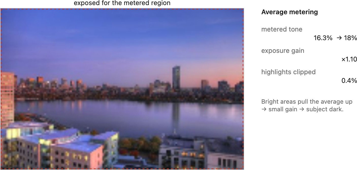
The metering connection is concrete. A reflected-light meter cannot tell whether a weak signal came from low illumination or a dark subject. Measuring a gray card of known reflectance under the subject's light removes one unknown from that comparison. An incident meter measures the arriving illumination instead of relying on the subject's reflectance. Both approaches help avoid brightening a black subject merely because it is black. They still require representative lighting and an exposure compatible with the range the camera can capture.
These coordinates discard scale: doubling the light leaves $x,y$ unchanged. Black has undefined chromaticity. Given $xyY$ with $y>0$, recover $X=xY/y$ and $Z=(1-x-y)Y/y$. Thus chromaticity plus luminance specifies the original tristimulus values; chromaticity alone does not.
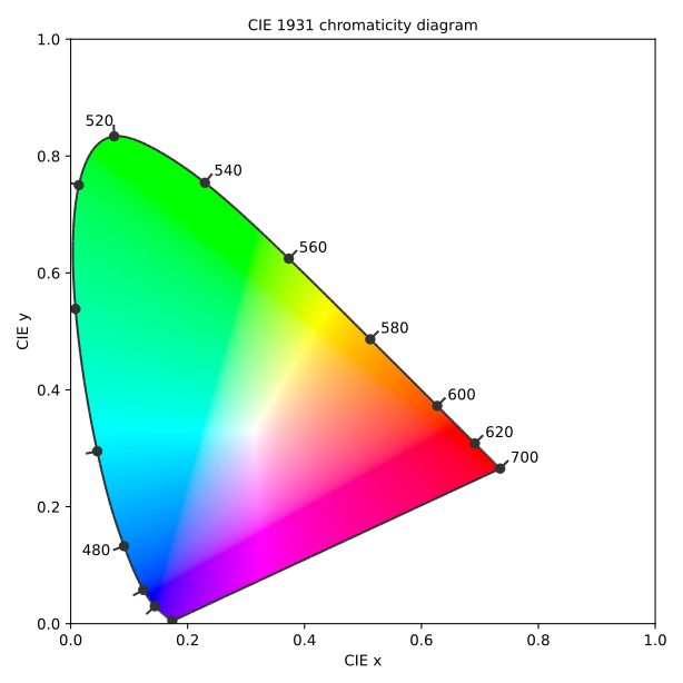
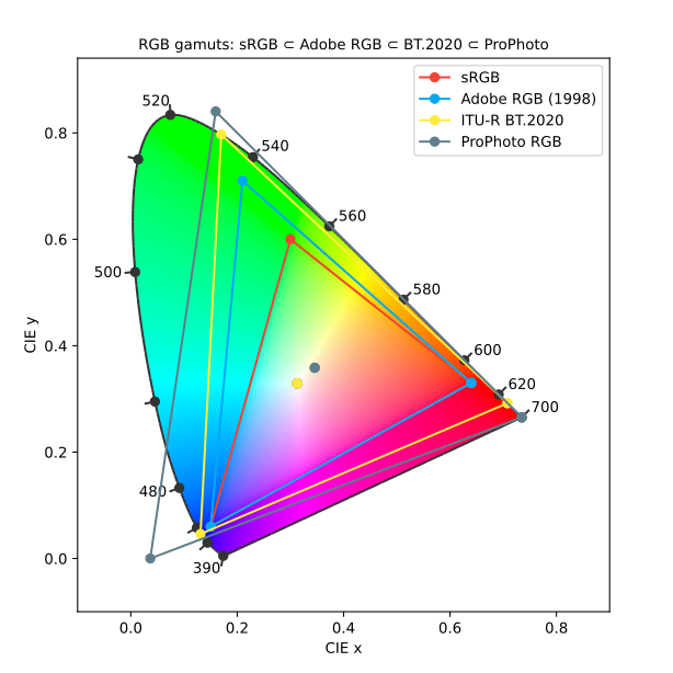
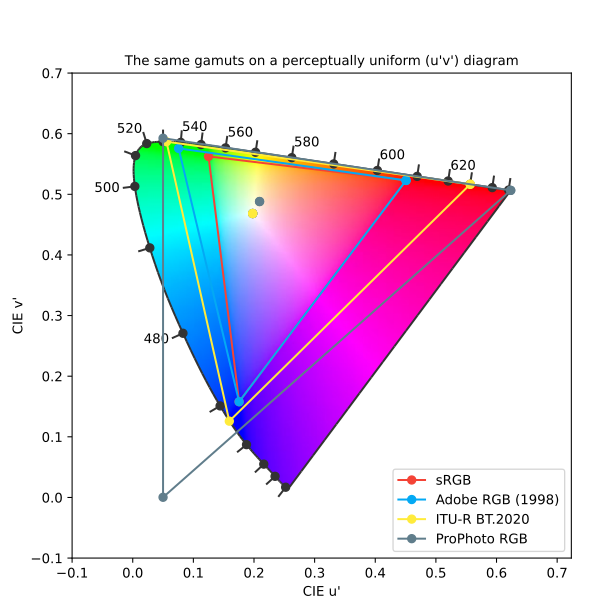
Monochromatic lights trace the spectral locus. Nonnegative mixtures lie in its convex hull, closed by the line of purples. The reference white is a selected point within this region, not an intrinsic center of the diagram. Euclidean distance in $xy$ is not a perceptual color difference.
Figure 4.1.7(reproduced). The CIE $xy$ chromaticity diagram. The horseshoe boundary is the spectral locus (pure monochromatic wavelengths, labeled in nanometers); the straight base is the line of purples. All physically realizable chromaticities lie inside; the white point sits near the center. Brightness has been divided out, so this is a map of hue and purity only (chromaticity).
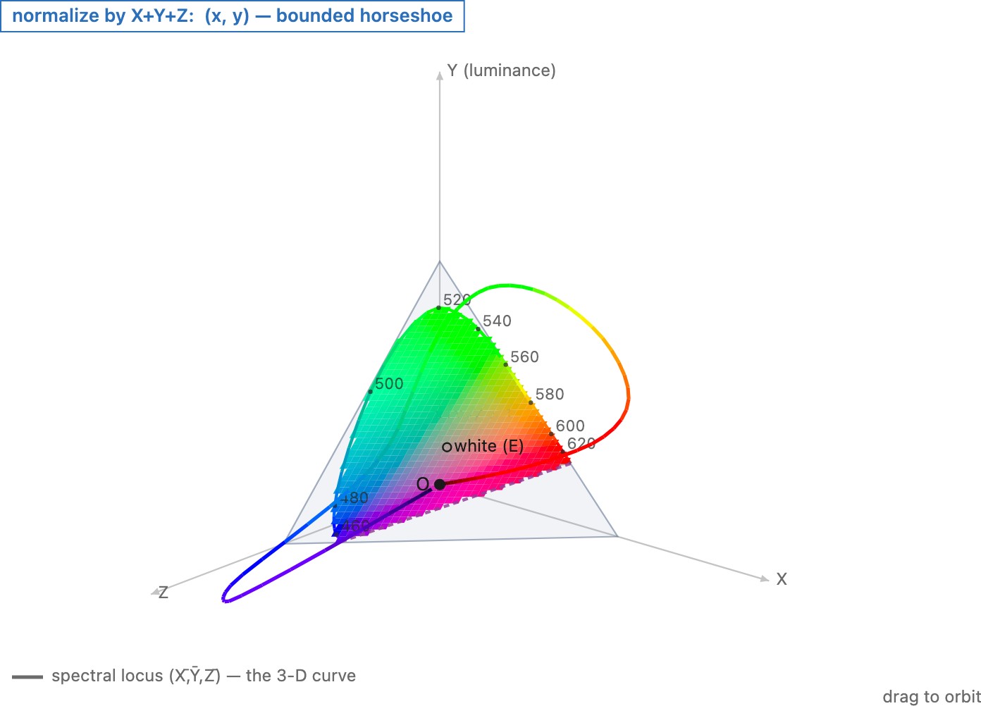
Geometrically, nonnegative spectra project to a cone of realizable tristimulus values Koenderink, Color for the Sciences. Normalizing by $X+Y+Z$ intersects each nonzero ray with a plane. Normalizing by another linear quantity gives a different cross-section. Although the underlying three-dimensional coordinates are related linearly, the normalized two-dimensional coordinates are related projectively.
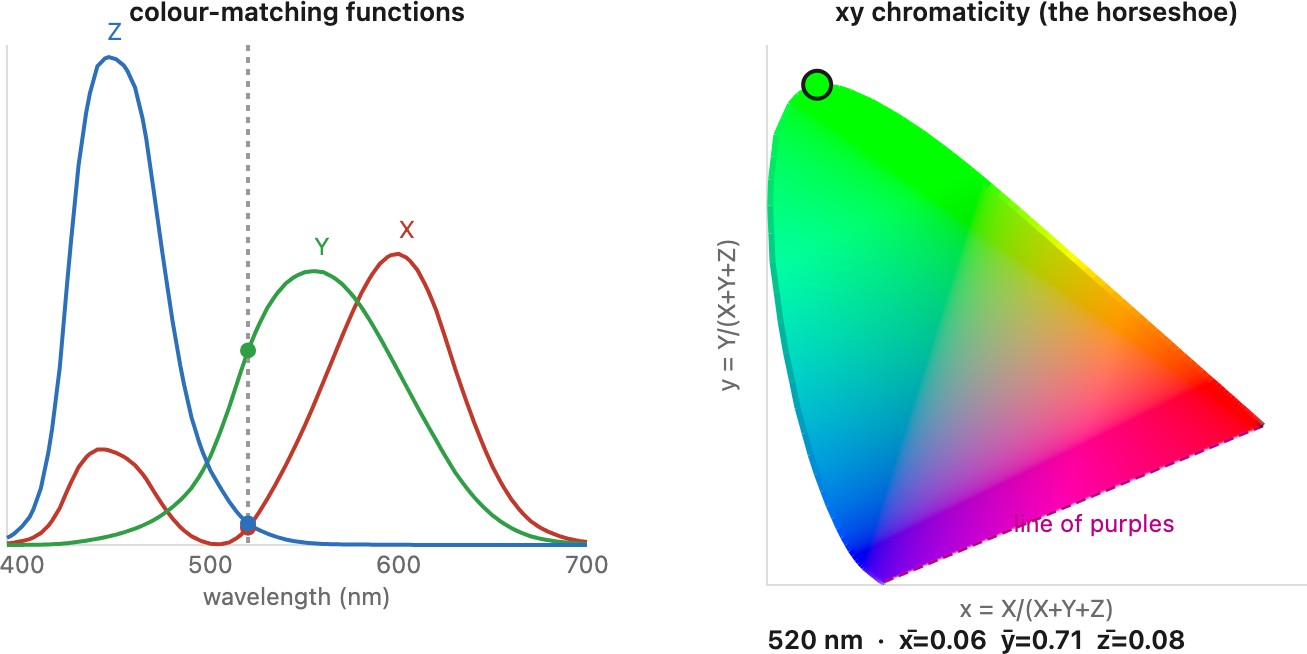
Figure 4.1.8(reproduced). The chromaticity diagram as a flat cross-section of Koenderink's 3-D cone, orbitable. CIE $XYZ$ space is drawn with luminance $Y$ vertical; the spectral locus is the 3-D curve of the color-matching values $(\bar X, \bar Y, \bar Z)$, and rays from the origin $O$ through it sweep out the cone of all realizable colors. A normalization plane slices that cone, and where each ray pierces it is the flattened chromaticity point. With the default plane $X+Y+Z=1$ (the Maxwell triangle) the slice is the familiar bounded, colored horseshoe: brightness divides out and every color lands in a finite region. Tick "normalize by just Y" to slice with the plane $Y=1$ instead, dividing by luminance alone: the coordinates $(X/Y, Z/Y)$ run to infinity as $\bar Y$ falls to zero at the spectral violet and red ends, so that chart is unbounded. That is exactly why the standard normalizes by the sum rather than by $Y$.Figure 4.1.9(reproduced). The chromaticity horseshoe, interactive, and where it comes from. It opens on the familiar CIE $xy$ ($XYZ$) view: left, the CIE color-matching functions; right, the spectral locus in $xy$ chromaticity, the curved horseshoe colored by wavelength, its interior filled with the actual color at each chromaticity, and closed along the bottom by the line of purples. Slide the wavelength and the same monochromatic light lights up on both panels. Switch the frame to LMS to swap the color-matching functions for the three cone sensitivity curves and the $xy$ diagram for the cone-response chromaticity ($l = L/(L+M+S)$, $m = M/(L+M+S)$): there the locus is the curved rim of the cone of all spectra (Koenderink), and its curve is literally the shape of the cone sensitivities. The two frames are just a linear transform of each other, so the horseshoe keeps its shape and only the coordinate frame changes. The third frame, MacLeod-Boynton, is the one that looks different, because it divides by something else. Instead of the sum of the three responses it divides by luminance: $l = L/(L+M)$ across, $s = S/(L+M)$ up, on the Smith-Pokorny fundamentals, which are scaled so that $L+M$ is exactly $V(\lambda)$. Every point in that plane is then the same brightness, a horizontal move is a pure trade of $L$ against $M$ and a vertical move is pure $S$, so the two axes are the two chromatic opponent mechanisms rather than an arbitrary pair of coordinates. The locus collapses onto the bottom edge for everything past about 520 nm, which says something real: beyond the green, wavelength barely moves the $S$ cones at all, and hue is carried almost entirely by the $L$ against $M$ balance.
MacLeod–Boynton chromaticity MacLeod & Boynton, cone-excitation chromaticity diagram (1979) uses cone fundamentals scaled so their L and M components sum to the luminance function. It plots $l=L/(L+M)$ and $s=S/(L+M)$. To interpret a horizontal displacement as an L–M trade at fixed luminance, hold the omitted scale $L+M$ fixed. The coordinates themselves do not force all plotted stimuli to have equal luminance, just as $xy$ does not.
A positive XYZ or LMS triple need not be physically realizable: positivity of three projections is weaker than existence of a nonnegative spectrum producing them. Reflectance introduces further constraints, since it must lie between zero and one under a specified illuminant. Do not confuse this surface-color problem with unconstrained emission.
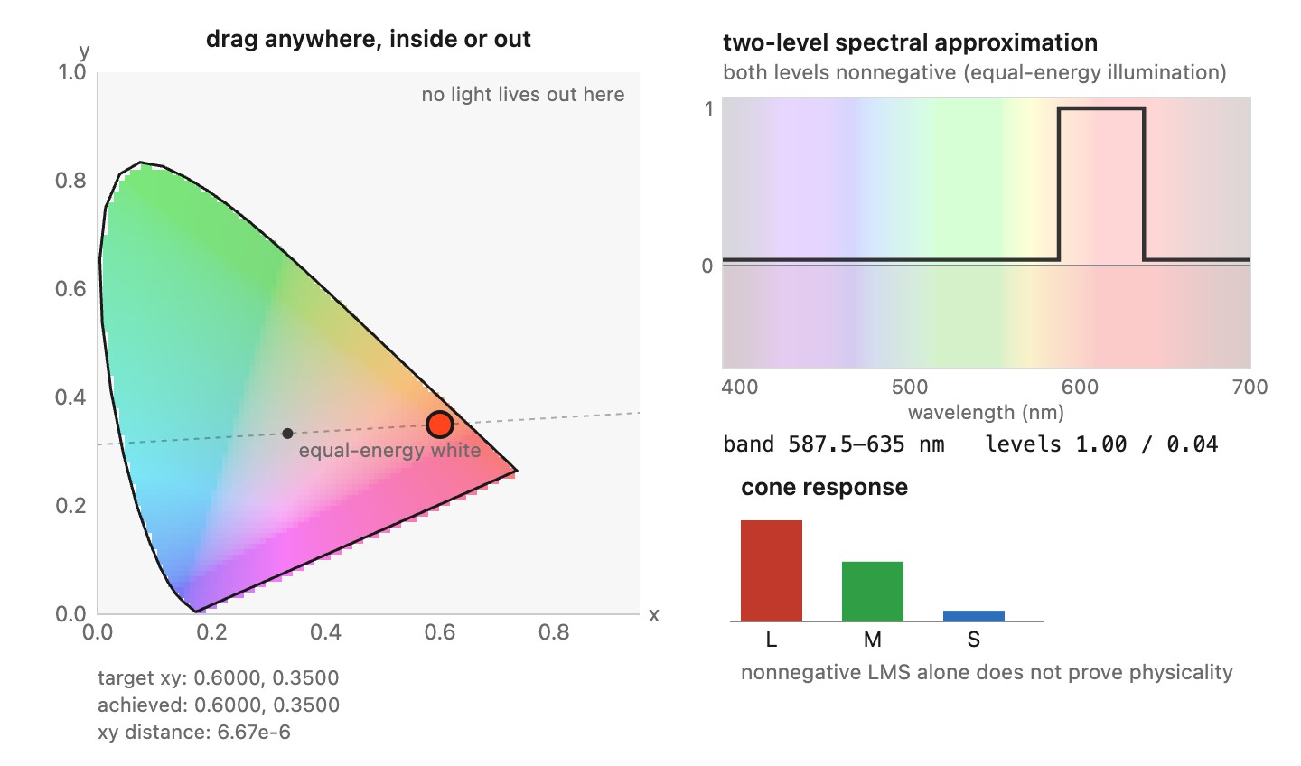
Figure 4.1.10(reproduced). What spectrum would it take to make this color, interactive. The previous figure says where the boundary is; this one says what the boundary means. Drag the point anywhere on the diagram, including outside the horseshoe. Inside, the answer is an ordinary reflectance, and the figure shows one: a two-level step, high on a band of wavelengths and low outside it, which is Schrödinger's optimal color whenever the low level comes out at zero. Outside the horseshoe no such spectrum exists, and rather than refuse, the figure shows the one you would need: one of the two levels goes below zero, and so does one of the three cone responses. That is the entire content of the word non-physical, and it is far easier to believe after watching the level cross zero as the point crosses the locus. The search is exact rather than fitted. For a fixed band, the chromaticities reachable by varying the two levels are precisely the straight line through equal-energy white and that band's own chromaticity, drawn dashed through the point, so finding the spectrum means finding the band whose line runs through the target and then solving for the levels. Every point on the plane lies on some such line, which is why the figure always has an answer; whether that answer is non-negative is exactly the question of whether the point is inside the horseshoe. The vertical scale puts the larger level at 1, so what changes as you drag is the sign, not the size.
Why divide by the sum rather than by luminance alone? Dividing by $Y$ is an appealing choice when the goal is to separate luminance from color, but coordinates such as $X/Y$ can become very large when $Y$ is small compared with another component. By dividing nonnegative XYZ coordinates by their sum, we instead put each normalized component between zero and one and make the three sum to one. The resulting diagram is bounded. This is a practical benefit of the chosen normalization, not a statement that its distances are perceptually uniform. Figure 4.1.8 makes the choice visible as a change of slicing plane.
The curved locus also has a physical origin. Sweep a monochromatic test through wavelength. At each setting its position comes from the three matching-function values at that wavelength, normalized by their sum. Those values vary together along the sensitivity curves, so the plotted point follows a curve rather than the sides of a triangle. Mixtures fill the convex region determined by that locus. The diagram's outline reflects the observer's spectral sensitivities; it is not an arbitrary shape chosen for a plotting convention.
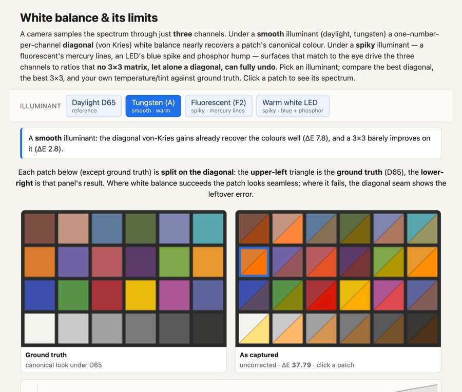
Two illuminants can have the same white chromaticity yet render colored objects differently. If a source delivers little or no energy in bands that distinguish two reflectances, three channel gains cannot recover the missing distinction. Even smooth illuminants need not be related by an exact diagonal correction.
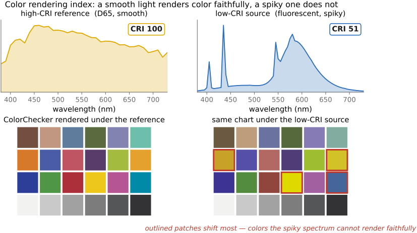
The color rendering index (CRI) compares specified test colors with a reference source at a similar correlated color temperature. The commonly quoted general index $R_a$ averages eight test colors; it is not a complete assessment of saturated colors, preference, or camera fidelity. A high score does not specify the illuminant spectrum. Contemporary lighting specifications may also report more detailed fidelity and gamut measures. For photographic work, examine the actual source and the materials that matter, especially when mixing lights.
Figure 4.2.5(reproduced). High versus low color rendering index. A ColorChecker chart rendered under a high-CRI reference (D65, CRI 100) and under a low-CRI spiky fluorescent (the CIE standard "F-series" fluorescent illuminant number four, CRI $\approx 52$), each white-adapted so the neutrals stay neutral, so the chromatic distortion is what shows. Both spectral power distributions and CRI scores are printed; the patches the spiky spectrum mis-renders are outlined. White balance keeps the grays true but cannot recover the colors the gappy spectrum never lit.Figure 4.2.6(reproduced). The limits of white balance, interactively. A Macbeth ColorChecker is rendered from spectral reflectances under a chosen illuminant (daylight D65, tungsten A, a spiky fluorescent, or a warm-white LED; the fluorescent is a synthetic spectrum with peaks at 430, 490 and 570 nm, not CIE F2, and the camera channels are XYZ converted to linear sRGB, not measured sensor sensitivities). The demo shows the captured chart beside the D65 ground truth, the selected patch's resulting spectrum, and the best correction by a diagonal (von Kries) gain versus a full $3\times3$ matrix, each fitted by least squares in linear RGB, with the mean CIE76 $\Delta E$ printed after gamut clipping, plus manual temperature/tint sliders. Smooth illuminants usually correct well, though not always exactly; spiky ones tend to leave a residual that no $3\times3$ removes. A nonzero residual alone does not identify a particular metameric pair; it shows that three gains or nine coefficients cannot undo a change that happened wavelength by wavelength.
A matrix fitted on chart patches can reduce their residuals without accurately correcting other materials. Separate fitting and evaluation sets when testing a camera transform. Neither a low training error nor a neutral gray row establishes general spectral recovery.
Linear image values are proportional to the measured or represented light. An encoding maps them to stored numbers. The choice matters both for precision and for processing: adding encoded values generally does not add the corresponding light.
Uniform integer steps in linear light devote relatively few levels to dark regions. Human contrast sensitivity often depends more closely on relative than absolute differences, so a nonlinear encoding can use a limited bit budget more effectively Poynton 2012. This is an engineering approximation, not a universal law of brightness. Visibility also depends on the background, spatial structure, noise, and viewing conditions.
For example, a range of 100:1 divided into successive one-percent ratios needs about $\ln(100)/\ln(1.01)\approx463$ intervals. This motivates allocating codes by relative precision, but it does not prove that eight bits always suffice. Smooth gradients and subsequent editing can expose eight-bit quantization.
The name “gamma correction” encourages the wrong mental model. An encoding changes the numbers used to represent light; decoding reverses that change. There may also be a display nonlinearity to compensate and a deliberate contrast change to apply, but these are separate jobs even when all three involve power curves. Poynton's discussion emphasizes the continuing value of perceptual encoding after the original CRT motivation Poynton 2012. Removing an old display technology does not remove the need to allocate a finite code range according to visibility.
An RGB space chooses primary chromaticities and a reference white; its stored representation also specifies a transfer function. Different choices serve different devices and workflows. sRGB is a common SDR delivery space. Display P3 extends its red and green coverage. Adobe RGB extends especially into greens and cyans useful in some print workflows. Rec. 2020 has still wider primary chromaticities. ProPhoto is a large working space with imaginary primaries.
With fixed integer precision, a larger gamut generally spreads codes more widely in color. The effect varies across the gamut and depends on the transfer function. Use sufficient precision for editing, then choose the delivery space from the output requirements. A screen cannot display every working-space value merely because software can store it.
Figure 4.4.1(reproduced). The choice, as a photographer meets it. Lightroom's export panel asks for a color space alongside the file format and the JPEG quality, and the menu is the zoo of this chapter: sRGB for the web and for anyone whose screen you cannot know, Display P3 and Adobe RGB when the destination is wider, ProPhoto RGB and Rec. 2020 for editing and for delivery to displays that do not exist yet. Nothing in the pixel values says which one was meant, which is why the choice has to be recorded in the file and why getting it wrong shows up as color that is merely plausible rather than right. Screenshot of Adobe Lightroom Classic.
💡 Big lesson (L4.8) — there is no single RGB: gamut versus bit budget
Choose a working gamut large enough for the content and operations, with sufficient numeric precision. Choose a delivery space the receiving system can interpret. Wider primaries alone do not improve an image, and converting an sRGB image to a wider space does not recover colors previously clipped.
Display-oriented spaces describe a reference set of primaries. Working spaces can instead choose imaginary primaries to enclose more physical colors. ProPhoto’s green and blue are outside the spectral locus; its red is not the imaginary pair’s other member. Such coordinates are useful for calculation, but their nonnegative cube contains values no physical light can produce.
Camera raw is different. Its channels are spectral measurements, often one color sample per photosite in a mosaic, not weights of three emission primaries. A camera would admit an exact universal XYZ matrix if its sensitivities spanned the standard observer’s matching functions. Real cameras generally only approximate this condition, so color correction is fitted and depends on spectra and illumination. It is not meaningful to invert an arbitrary three-by-many sensitivity matrix and call the result three physical display primaries.
Camera profiles can provide multiple illuminant calibrations. Do not assume every DNG contains exactly two matrices at fixed temperatures; use the tags and conventions of the actual profile. Camera color-space menu settings usually govern rendered output and previews, while raw channel interpretation remains camera-specific.
The correction matrix also propagates noise. With equal independent input variances $\sigma^2$, output channel $i$ has variance $\sigma^2\sum_j M_{ij}^2$. More generally use $M\Sigma M^T$. Negative coefficients do not alone prove amplification; their magnitudes and the input covariance matter. The filter design and color fit balance sensitivity, color accuracy, and noise, as developed in Chapter 4.6, Sensing color: multiplexing strategies.
Figure 4.4.2(reproduced). RGB primaries on the chromaticity diagram. The triangle vertices are the red, green, and blue primaries of each space, and the triangle they enclose is that space's gamut. sRGB / Rec. 709 is the small triangle, and Adobe RGB, Rec. 2020 and ProPhoto enclose progressively larger areas: each really does contain the one before it, primary by primary. ProPhoto is the one to look at twice. Two of its three primaries lie outside the spectral locus, so they are not colors at all, and a corner of its triangle names nothing that can be seen. A change of space is a $3\times3$ matrix between these triangles.Figure 4.4.3(reproduced). The same RGB gamuts on a perceptually uniform diagram. The identical sRGB, Adobe RGB, BT.2020 and ProPhoto primaries of the previous figure, replotted on the CIE 1976 UCS ($u'v'$) chromaticity diagram, which spaces colors far more evenly by perceived difference. Compared with the $xy$ diagram, the oversized green lobe collapses and the blues open up, so the triangles take on very different shapes and relative areas, from the very same numbers. The lesson: $xy$ (and $XYZ$) measures color, it does not tell you how different two colors look. Rendered by colour-science.Figure 4.4.4(reproduced). Chromaticity and color spaces, interactive. Every gamut is drawn at once on the CIE horseshoe, faintly, and one is selected from the row of buttons: that one is drawn in full, carries the draggable handles, and drives everything else. Selecting it also sets the encoding that space is really used with, sRGB, Adobe RGB and Display P3 at $\gamma \approx 2.2$ in 8 bits, Rec. 2020 at 2.4 in 10, ProPhoto at 1.8 in 16; both sliders stay free afterwards. The axes run a little below zero so a primary can be dragged outside the locus, which is where two of ProPhoto's live. A checkbox swaps $xy$ for the perceptually uniform $u'v'$ diagram, and the coverage readout is measured in $u'v'$ either way: sRGB holds 33.3% of the visible chromaticities, Adobe RGB 38.8% (1.17× sRGB), Rec. 2020 57.4% (1.72×), ProPhoto 76.7% (2.30×), and the editable triangle live as you drag it. Below the diagram, what quantization costs in that space. At every code in the space's own cube, step one level along $R$, $G$ and $B$, decode both ends through that space's transfer and that space's primaries, and measure the step as a full CIELAB $\Delta E$, lightness and chroma together and not brightness alone; the histogram is the distribution of those steps, and 1 $\Delta E$ serves as a rough proxy for a just-noticeable difference, which in practice varies with the color and the viewing conditions. Its axis is fixed, $0.001$ to $10\,\Delta E$, so two spaces can be compared by eye rather than by reading the ticks; steps past either end are counted into a bar outside the axis instead of being squeezed in. It answers to all three knobs. Widen the primaries and the same codes have more color to cover: at 8 bits and $\gamma = 2.2$, 0.3% of sRGB's code steps are visible, against 8.0% for Rec. 2020 and 23.3% for ProPhoto, which is exactly why ProPhoto is specified at 16, where it is back to 0.0%. Change $\gamma$ instead, in sRGB at 8 bits, and you get the other half of the story: 6.5% of steps visible at $\gamma = 1$, 0.3% at 2.2, none at 3.0, while the median step grows. Gamma does not remove the error, it levels it. Underneath, the dynamic range those same codes buy, from the dimmest non-black code up to white: 8.0 stops at $\gamma = 1$, which is one stop per bit and no more, against 17.6 at $\gamma = 2.2$ in the same 8 bits, 24.0 for Rec. 2020's 10 bits at 2.4, and 28.8 for ProPhoto's 16 at 1.8. Unlike the histogram, that number is set by the encoding alone and not by the primaries, since every space here puts white at $Y = 1$. Read it as an upper bound: the slider is a pure power, whose slope at zero is infinite, so it reaches further into the dark than a real transfer curve with a linear toe. sRGB's actual piecewise curve gives 11.7 stops at 8 bits, not 17.6. On the right, one sample throughout, a measured reflectance cube rendered under D65, with every pixel the selected space cannot hold flagged. Only 2.4% of these paints leave sRGB, 0.6% leave Display P3 and none leaves Rec. 2020, which is this section's argument in three numbers: real pigments barely need more than the oldest gamut.
This distinction explains two different kinds of color-conversion experiment. Between linear RGB working spaces built from the same standard observer, convert a color to XYZ and then to the destination coordinates; the two matrices compose into one exact coordinate transform. For a camera, photograph a set of known reflectances under a specified light and fit a matrix from the measured camera responses to their target XYZ values. It can fit those samples well and still make errors on other spectra. Two spectra that the camera records identically cannot be separated by any later matrix, even if the standard observer distinguishes them. More training patches improve the fit over a chosen population; they do not restore spectral information absent from the three measurements.
The choice of a working gamut also affects quantization. With a fixed integer bit depth, a wider set of primaries spreads the available code combinations over a larger range of colors. It can retain a saturated color that a smaller space clips, yet give coarser steps in a region shared by both spaces. Increasing bit depth or using floating point reduces that pressure. This is why a space suited to intermediate editing need not be the best choice for compact delivery. The working space must retain the colors the pipeline needs; the output space must match the interpretation supported by the destination.
A caution about that diagram before we read too much into the triangle sizes: the $xy$ chromaticity plane is a space for measuring color, not for judging how different two colors look. It stretches the greens enormously and cramps the blues and purples, so neither the relative areas of these gamuts nor the distances between their primaries track perceived difference. Re-plot the identical primaries on a perceptually more uniform diagram, the CIE 1976 UCS ($u'v'$) space, and every triangle changes shape (Figure 4.4.3): the relative areas and distances change. The newer diagram is more uniform, but it is still not a universal perceptual ruler. That $XYZ$ (and its $xy$ projection) is not perceptually uniform is precisely what will force the deliberately non-linear spaces of Chapter 4.5, Advanced color: opponents, perceptually-uniform, and preferred.
Two design processes can lead to an RGB space. In a display-oriented design, begin with the primaries a reference display can emit, then describe colors as amounts of those lights. In a working-space design, begin with the colors that editing should retain, then choose a coordinate system that encloses them. The latter need not correspond to a manufacturable display. An imaginary primary is acceptable as a coordinate axis because no lamp is being asked to emit it while the image is stored or edited. Physical realizability becomes an output constraint when those values are converted for a screen or printer.
This distinction explains why choosing a larger working space does not upgrade the monitor. It changes which intermediate colors can be represented without clipping to the working cube. Displaying them still requires conversion and, where needed, gamut mapping. Conversely, a delivery space can be chosen for compatibility with the intended viewing path even when a larger space was useful during editing. The export dialog asks for an engineering choice about that destination, not a ranking in which the largest triangle is always best.
The noise formula can be read numerically. A correction row with coefficients 1.8, -0.9, and 0.1 has squared length 4.06. With equal independent input noise, its output standard deviation is therefore about 2.01 times the standard deviation of one input channel. The row may improve the color fit while increasing that channel's noise. This is why a camera characterization should be evaluated for both reconstruction error and noise propagation, using the actual covariance rather than assuming that every color matrix has the same cost.
Advanced color: opponents, perceptually-uniform, and preferred⧉
Preferred colors: skin, sky, and other memory colors⧉
Viewers bring expectations to familiar objects, especially faces. A camera can produce a colorimetrically plausible image yet render a face in a way its subject dislikes. Skin rendering therefore requires both accurate measurement and a deliberate rendering objective.
The vectorscope’s conventional skin-tone line is a useful reference under some lighting and rendering conditions. It is not a universal target. Complexions, blood perfusion, body site, illumination, makeup, exposure, and camera processing all affect the measured hue. Pulling every face toward one line can remove real variation.
Figure 4.5.10(reproduced). The skin-tone locus. On a vectorscope, skin tones across a wide range of people cluster along a single line (the I axis, between red and orange), differing mainly in lightness and saturation, not hue. This tight locus is why colorists pull skin toward one reference line, and why cameras are tuned to render it well.
CIELAB skin measurements must specify their illuminant and observer. The individual typology angle Chardon et al. 1991 (ITA°) is a descriptor based on $L^*$ and $b^*$, conventionally expressed as $\mathrm{ITA}=\arctan((L^*-50)/b^*)$ in degrees in its intended domain. It discards $a^*$ and is not a complete color description. Do not infer a person’s complexion category from an uncalibrated JPEG or treat fixed hue limits as an inclusive skin detector.
Figure 4.5.11(reproduced). Skin tones in CIELAB (interactive). A schematic of the skin locus, from very light to very dark: the cloud is generated by a simple two-parameter formula in CIELAB with added jitter, not measured from skin. In the ITA° view ($L^*$ vs $b^*$) the individual typology angle $\mathrm{ITA}° = \operatorname{atan2}(L^*{-}50,\, b^*)$ cuts the locus into the conventional classes, at 55°, 41°, 28°, 10° and −30° from very light to dark; in the hue view ($a^*$ vs $b^*$) the tones cluster near a hue angle of about 50°, drawn as a reference ray, though real skin hue also varies with pigmentation, lighting and imaging. Two sliders mimic the two pigments that set skin color, melanin (darkens and yellows, in the epidermis) and hemoglobin (reddens, in the dermis) Tsumura et al. 2003; their values are not concentrations, and since the sliders and the cloud come from the same model, the synthetic color landing on the cloud is not independent validation. Interactive: switch between the ITA° and hue views, and move the melanin and hemoglobin sliders to place a synthetic skin color on the locus, reading off its $L^*a^*b^*$, ITA°, and hue angle.
Melanin and hemoglobin strongly influence skin reflectance, but skin is not exactly a two-parameter color surface. Hemoglobin oxygenation, layer thickness, scattering, and illumination also matter. Tsumura et al. Tsumura et al. 2003 estimate pigment-related image components using a model and statistical assumptions; arbitrary RGB attenuation vectors are not that calibrated method.
A physical forward calculation keeps the spectral integration explicit:
A log-RGB approximation can simplify separation under suitable conditions, but the logarithm of a spectral integral is not the integral of a logarithm. Label any reduced model and validate it against measured spectra. For spatially resolved rendering, subsurface scattering also matters: a BSSRDF relates entering light at one surface point to exiting light at another. Chapter 35.5, Light domes develops computational capture for face relighting.
Historical calibration choices also mattered. Shirley reference cards and film practices centered light-skinned subjects, contributing to poor rendering of darker skin Roth 2009 (the Shirley card). Evaluate capture, exposure, noise, and rendering across the people and conditions the system must serve, instead of assuming a reference face represents everyone.
Video 3. Vox’s account of Shirley cards and the history of skin-tone reproduction.
Memory-color studies also examine sky and foliage. Preferred reproduction can differ from measured color, but it varies with context, observers, and the intended image. A blue swatch alone does not establish that a pixel is sky, just as a warm swatch does not establish skin. Preferred-color edits need semantic context and should preserve distinctions that matter to the photograph. There is no universal table of Lab prototypes that defines correct skin, sky, and vegetation.
A small RGB attenuation model lets us inspect the algebra behind the two-factor construction. The coefficients below are chosen for illustration. They are not measured absorption spectra, and the result is not an implementation of Tsumura et al.'s calibrated separation method. Spectral integration and scattering prevent a general identification of RGB logarithms with physical pigment densities.
Listing 1 · illustrative attenuation and color conversionembed
import numpy as np
# --- linear sRGB (D65) -> XYZ -> CIELAB, and linear -> sRGB --------------
M_RGB2XYZ = np.array([[0.4124, 0.3576, 0.1805],
[0.2126, 0.7152, 0.0722],
[0.0193, 0.1192, 0.9505]])
WHITE = np.array([0.95047, 1.0, 1.08883]) # D65 reference whitedef srgb_encode(lin): # linear light -> sRGB, [0,1]
lin = np.clip(lin, 0.0, 1.0)
return np.where(lin <= 0.0031308, 12.92*lin, 1.055*lin**(1/2.4) - 0.055)
def lin_rgb_to_lab(lin): # linear light -> CIELAB
t = (M_RGB2XYZ @ np.asarray(lin, dtype=float)) / WHITE
d = 6/29
f = np.where(t > d**3, np.cbrt(t), t/(3*d*d) + 4/29)
return np.array([116*f[1] - 16, 500*(f[0]-f[1]), 200*(f[1]-f[2])])
# Illustrative two-factor attenuation in RGB, not a calibrated skin model.# These chosen vectors demonstrate log products becoming sums; their# parameters are dimensionless controls, not measured pigment concentrations.
RGB_BASE = np.array([0.95, 0.88, 0.80]) # chosen baseline (linear RGB)
SIGMA_MEL = np.array([0.35, 0.60, 1.00]) # melanin: absorbs blue > green > red
SIGMA_HEM = np.array([0.12, 0.85, 0.80]) # hemoglobin: absorbs green (540-580 nm) + bluedef skin_linear(melanin, hemoglobin): # nonnegative illustrative controls
v = np.log(RGB_BASE) - melanin*SIGMA_MEL - hemoglobin*SIGMA_HEM
return np.clip(np.exp(v), 0.0, 1.0) # linear-light RGBdef skin_srgb(melanin, hemoglobin): # -> display sRGB, [0,1]return srgb_encode(skin_linear(melanin, hemoglobin))
def skin_lab(melanin, hemoglobin): # -> CIELAB (D65)return lin_rgb_to_lab(skin_linear(melanin, hemoglobin))
Increasing either nonnegative control reduces the linear channels according to its coefficient vector. In log RGB the two changes add; exponentiation returns to linear RGB before conversion to CIELAB or display encoding. This example shows the computation and its domains without claiming that two parameters span all skin appearance.
The other useful implementation is a color-region selector. The region must be chosen for the editing task; there is no universal CIELAB box that identifies skin, sky, or vegetation. Hue intervals can cross zero, and neutral pixels need separate handling:
Listing 2 · an explicitly chosen CIELAB regionembed
import numpy as np
def in_lab_region(lab, lightness_range, hue_range, chroma_range):
# A geometric selection in CIELAB, not an object classifier.
L, a, b = lab
chroma = np.hypot(a, b)
if chroma == 0:
returnFalse# hue is undefined on the neutral axis
hue = np.degrees(np.arctan2(b, a)) % 360
lo, hi = (v % 360for v in hue_range)
inside_hue = lo <= hue <= hi if lo <= hi else hue >= lo or hue <= hi
return (lightness_range[0] <= L <= lightness_range[1] and
chroma_range[0] <= chroma <= chroma_range[1] and inside_hue)
# Arbitrary warm-color box for an editing experiment, not a skin-tone standard.
selected = in_lab_region([60, 20, 20], (20, 90), (20, 70), (5, 60))
A warm wall and a face can both satisfy this test. Combine a color selection with spatial or semantic evidence when the intended adjustment concerns an object. Using a geometric region for a selective edit is different from claiming that it recognizes the material.
The pigment model is useful because the two major absorbers do different things. Melanin in the epidermis absorbs broadly; increasing it tends to darken the reflected signal. Hemoglobin in dermal blood has a more structured spectrum and helps determine the reddish component and changes associated with perfusion. Light can pass through both regions and scatter before leaving the skin, so their effects combine along its paths. The simplified log model turns multiplicative attenuation into additive components, making separate controls convenient. Its usefulness does not make the fitted RGB components direct physical concentration measurements.
Subsurface transport adds a spatial effect. Light entering at one point can emerge nearby, so the color at that exit point depends on illumination over a neighborhood. A local surface-only model misses this redistribution even if its color parameters are correct. Controlled illumination in a light stage helps measure how a face responds as the incident direction changes, providing evidence for relighting models. Color calibration, pigment approximation, and spatial scattering address different parts of why the rendered face looks convincing.
The response includes filters, optics, and quantum efficiency under the stated convention. Sampled implementation needs wavelength-bin weights. Shot noise is determined by detected electrons, while read noise is added by the readout; the full model is in Chapter 2.8, Noise, signal-to-noise ratio and dynamic range. A broad response alone is not a color measurement: distinct response shapes supply the information that separates spectra.
The exact shape of a color sensor's three spectral-sensitivity curves (the $r(\lambda)$ of the red, green, and blue channels, built earlier by the color-filter array on the photosites of Chapter 2.7, Sensors: photosites, CCD vs CMOS) is one of the camera's most constrained choices, because it is pulled in three directions at once that cannot all be satisfied.
Fidelity to human vision. For a camera to record the color a human would see, its three curves should be a fixed linear combination of the eye's cone fundamentals (equivalently, of the CIE color-matching functions), the Luther–Ives condition. A sensor that met it could be mapped to human color by a single $3\times3$ matrix with no error. Practical camera sensitivities generally only approximate it, because silicon-plus-dye curves are simply the wrong shape, and the penalty is a metameric error no color matrix can remove: two spectra that look identical to the eye read as different RGB, and two that look different can read the same. The color-correction matrix in Chapter 8.10, Auto-exposure and auto white balance is a least-squares compromise: right on average, wrong on the hard cases (saturated reds, narrow-band LEDs, foliage).
Quantum efficiency and noise. Broad transmission bands can increase total photon collection; this is distinct from quantum efficiency at a specified wavelength: the wider each filter, the more photons reach the well and the higher the SNR. Strong overlap can make color separation poorly conditioned, because separating similar channel responses can require large signed coefficients that amplify measurement noise (compare the distinct physiological opponent processing in Chapter 3.2, Perceptual color and trichromatic vision). Narrow, well-separated filters give clean color but throw photons away and read noisier. The green-doubled Bayer is one point on this curve: spend photons and resolution where the eye cares most (luminance), economize on chroma.
White balance across illuminants. Because each channel integrates illuminant × reflectance × sensitivity, changing the light changes the raw RGB of a fixed object. Undoing that, white balance often approximates the change with per-channel gains. Matching cone sensitivities does not make this diagonal relighting model exact; a response set that matches human colorimetry well need not be the best basis for diagonal adaptation. Good spectral design makes white balance more reliable across illuminants (→ Chapter 8.10, Auto-exposure and auto white balance).
These three pull against each other: the curves that best match the eye are broad and overlapping (bad for separation), the curves that separate color cleanly are narrow (bad for QE and for matching the eye), and keeping white balance stable across odd illuminants wants yet another shape. Every color sensor is a negotiated settlement among them (Figure 4.6.24).
Figure 4.6.24(reproduced). The spectral-sensitivity trilemma. (a) Match the eye: the human cone fundamentals (smooth, heavily overlapping) beside a real sensor's RGB, the mismatch (the sensor is not a linear transform of the cones, the Luther–Ives condition) is the metameric error no color matrix can undo. (b) Photons vs separation: narrow filters separate color cleanly but pass few photons (low quantum efficiency, noisy); broad filters catch far more light (shaded area) but overlap so heavily that recovering color means differencing correlated channels and amplifying noise. (c) Tunable nanocrystals: a colloidal quantum-dot layer's absorption peak shifts with dot size (quantum confinement), so spectral sensitivity becomes a design parameter: sharper, higher-absorption, and extendable into the infrared and ultraviolet. Schematic.
Recap: the full color pipeline, color management and ICC optional⧉
ICC profiles describe transforms between device or encoding values and a profile connection space (PCS). In the conventional ICC v2/v4 architecture, that space uses D50-referenced XYZ or Lab. A color-management module combines source and destination transforms. Profiles can use matrices and curves or multidimensional lookup tables; a printer is not generally one three-by-three matrix away from RGB.
Figure 4.8.1(reproduced). The ICC color-management workflow. An image's device-dependent values pass through the source device's profile into a device-independent profile-connection space (PCS, $XYZ$ or CIELAB), then through the destination device's profile into its values. Every device-to-device move routes through the PCS, so each device need only know how to talk to the common space.
Assigning a profile declares the meaning of unchanged values. Converting profiles changes values to meet a color-reproduction objective. For example, the triple $(0.8,0.2,0.1)$ denotes different colors in sRGB and Adobe RGB. Assigning Adobe RGB to sRGB data leaves that triple unchanged and changes its interpretation. A conversion starts with the sRGB interpretation and computes destination values for the intended match, subject to the destination gamut and rendering intent. Assign the known source interpretation before conversion. For an untagged image of uncertain origin, sRGB is a common fallback assumption, not recovered metadata.
Intent
Objective and limitation
Media-relative colorimetric
Relate source white to destination white and retain in-gamut colorimetry relative to those whites. Out-of-gamut behavior depends on the conversion.
ICC-absolute colorimetric
Retain source media-white colorimetry, useful for proof simulation; destination limits still apply.
Perceptual
Re-render colors to accommodate differences between media, potentially changing in-gamut values. The mapping is profile- and implementation-dependent.
Saturation
Favor vivid graphic reproduction over strict colorimetric matching; behavior is profile-dependent.
Black-point compensation is a separate option that maps tonal ranges between different black points, commonly used with relative colorimetric conversion. Compare it with the selected profiles instead of treating it as another rendering intent. See the ICC introduction and black-point compensation white paper.
Profile construction and connection account for chromatic adaptation. Bradford is widely used in this architecture Bradford chromatic-adaptation transform, but do not prepend an extra adaptation to an already specified profile conversion. The complete Bradford formula and its white-to-white checks are in Chapter 4.2, White balance and white point. A camera’s raw gains are not simply that same XYZ transform.
For printing, use the profile matching the actual printer, ink, paper, and driver settings. If the application converts to printer values, configure the driver accordingly; if the driver owns conversion, supply the input it expects. A printer profile should not be embedded as though it described an ordinary web RGB image.
For an unchanged scene and lens transmission, optical exposure scales as
$$H\propto \frac{t}{N^2},\qquad N=\frac{f}{D}.$$
Twice the integration time collects twice the light. Multiplying the f-number by $\sqrt{2}$ halves it. Thus f/2.8 at 1/250 s and f/4 at 1/125 s give approximately the same optical exposure, but the longer integration blurs motion more and the smaller aperture increases depth of field.
A stop is the base-two logarithm of a light ratio. The setting-based exposure value uses time in seconds:
Increasing this EV by one halves optical exposure. Positive exposure compensation is a different convention: it asks an automatic mode for a brighter result relative to its metered choice. In aperture priority at fixed ISO, +1 stop will ordinarily double time. In manual mode with Auto ISO it may instead double gain while leaving the light collected unchanged.
ISO is not a third optical control. At fixed aperture and time, increasing gain scales the signal and its shot noise together. It can reduce the importance of noise added downstream of that gain, or select a sensor conversion-gain mode with lower input-referred read noise. It can also reduce highlight headroom. On an ISO-invariant sensor over the relevant range, low-ISO raw data brightened later can be close to a higher-ISO capture. The comparison in Chapter 2.8, Noise, signal-to-noise ratio and dynamic range applies only after matching output brightness and checking clipping.
The common association between high ISO and noise usually includes a reduction in collected light: we raise ISO because the scene is dim or the shutter must be fast. Add light, open the aperture or lengthen time when the photograph permits it. Raising ISO alone does not improve photon statistics.
Reflected-light metering measures light coming from the scene; it cannot separate a dark object in strong light from a pale object in weak light without additional information. Spot metering makes the chosen patch explicit. Evaluative metering uses more of the frame and may use recognized subjects. A gray card is a useful reference under the subject's illumination, not proof that a meter assumes exactly 18% reflectance. Snow and dark clothing are good tests of when compensation is needed.
Expose to the right means collecting more light while retaining the highlights that matter. It is useful when time, aperture and saturation allow it; it is not a requirement to force every histogram against the edge. A longer exposure that blurs the subject is a poor trade for cleaner shadows. Inspect individual channels when possible, because a colored light can saturate one channel before the luminance preview looks white. Keep a margin when the camera's warnings refer to a processed preview rather than raw data.
💡 Big lesson (L5.1) — photographers measure light in stops
A stop is a factor of two. Time steps by two and f-number by $\sqrt{2}$. ISO and a software exposure slider can change rendered brightness by a stop without collecting another photon.
The f-number normalizes the physical opening by focal length. At the same f-number, a longer lens has a proportionally larger entrance pupil. For an extended scene of equal radiance, that compensates for the change in image scale so the on-axis irradiance is approximately unchanged, apart from transmission and close-focus effects. Aperture diameter alone would not give that useful comparison across focal lengths.
The familiar series f/1.4, f/2, f/2.8, f/4, f/5.6, f/8, f/11, f/16 follows from area. Each full-stop step multiplies the f-number by about the square root of two and therefore halves optical exposure at fixed time. Doubling time compensates for that step. For example, f/4 at 1/250 s and f/5.6 at 1/125 s collect approximately the same light per sensor area, with different motion blur and depth of field. Equal collected light does not make them interchangeable photographs.
Before built-in meters, exposure tables related film speed to illumination and subject conditions. A handheld incident meter measures light arriving at the subject, while a reflected meter measures light leaving a selected area. Through-the-lens metering accounts for some effects of the actual optical path. None of these devices knows which part of a photograph we intend to emphasize.
For repeatable work, meter a defined patch or use a controlled reference under the same illumination. Record compensation and whether settings were locked. Absolute photometry requires more than the settings printed in EXIF; Chapter 17.2, Camera response and radiance calibration develops that distinction.
Figure 5.2.11(reproduced). Before light meters, an exposure table. The back plate of a Rolleiflex twin-lens reflex engraves an exposure guide: rows of lighting conditions (bright sun, cloudy, dull) against film speed, giving the aperture and shutter to use. The photographer read the scene by eye and looked up the settings, exactly the "sunny 16" idea made into a chart. (Photo Gisling, CC BY-SA 4.0, via Wikimedia Commons; see credits.)Figure 5.2.12(reproduced). A handheld light meter with both metering modes. The white dome (top left) reads incident light: held at the subject and pointed back at the camera, it measures the light falling on the subject over a hemisphere, independent of the subject's own tone, so it sidesteps the 18%-gray problem. The narrow spot viewfinder (the tube) reads reflected light: aimed at the scene, it measures the light coming off a chosen patch, which is what every in-camera meter does and why it is fooled by very light or very dark subjects. (Sekonic L-558R.)
A reflected reading changes when a gray card is replaced by a white card under the same light. If an automatic system treats the brighter reading as a reason to shorten exposure, it can render the white card too dark. An incident reading taken at the subject responds to the illumination instead of that change of card reflectance. The white card can then remain lighter than the gray one under the same exposure. This is the practical attraction of an incident meter in a controlled setup; it does not determine the photographer's desired rendering.
The cost is access. You can aim a reflected-light spot meter at a distant subject from the camera position. Taking an incident reading requires sampling the light at a representative subject position and choosing how to orient the receptor. Mixed lighting and directional sources make that choice consequential. Meter type changes which quantity is measured, not whether judgment is needed (Figure 5.2.12).
Printed exposure guides made the first choice without measuring the scene. Film packaging and exposure calculators listed settings for bright sun, overcast light, and shade. The sunny-16 rule summarizes one such starting point: in bright sun, use f/16 and a time near the reciprocal of the film-speed number, about 1/100 s for ISO 100. It is a lighting estimate, not a measurement of every subject or a guarantee against clipped highlights.
Photocells made the estimate responsive to actual light. A separate or body-mounted meter could still see a different field from the taking lens and miss the loss from an added filter. Through-the-lens metering brought the measurement into the optical path that forms the photograph, accounting for transmitted light. Sensor-based metering brings it closer still: the camera analyzes a live readout from the imaging sensor. Preview processing and capture settings can differ, but the remaining decision, which tones matter and where to place them, still requires an inference about the scene and the photographer's intent.
A face beside a window can have plenty of light and still photograph badly if the eyes fall into shadow. Move the subject or the source before changing exposure. Exposure scales the measurement; lighting changes the relationships within the scene.
Describe a source by its direction, apparent size, intensity, spectrum and timing. Direction places the shadows. Apparent size controls their penumbra. Intensity sets the photon budget and the balance with other sources. Spectrum affects color, and timing determines whether a flash freezes motion or a lamp produces bands. These properties are related in practice, but none substitutes for the others.
A large source can soften a shadow without filling it. Shadow contrast also depends on light arriving from other directions and on the surroundings. A small source can be useful for revealing texture or making a crisp graphic shadow. Soft light is a useful choice for many portraits, not a requirement for a good photograph.
Move a light sideways and the shadows move; enlarge it without changing its central direction and their edges soften. These are different changes. A small frontal source can make texture difficult to see because its shadows lie behind the relief from the camera's viewpoint. Raking side light reveals the same relief with visible shadows. A large source spans a range of directions, so a point near a shadow boundary can see part of the source while another part is occluded. That partial visibility produces the penumbra. A reflector, diffuser, or softbox should therefore be judged from the subject's position: what luminous area does the subject actually see?
Highlights provide another way to inspect the source. On a glossy object, their shape depends on both the source and the material's reflection function. A small bright source can produce a concentrated highlight; a broad source can produce an extended reflection. On glassware or a polished object, moving or enlarging the source can change the visible form more than changing exposure. Lighting controls the reflected image of the environment as well as the shadows cast onto the subject.
Direct on-camera flash can produce a small-source shadow and a strong frontal reflection, which may be exactly the desired appearance. For softer directional light, bounce off a suitable wall or ceiling. The illuminated area becomes the source seen by the subject. Its location, apparent size, color and distance matter; a distant dark ceiling can consume most of the available flash energy.
A small diffusion cap on a flash does little to enlarge the apparent source outdoors. Indoors it may spread light onto walls that then become larger sources. A softbox or scrim works through the illuminated area visible from the subject, so bringing it closer generally increases its angular size.
A white reflector redirects available light into shadows. A silver surface is more directional, and a colored surface tints the reflected illumination. A black panel removes fill. Move the panel while watching the face before adding another lamp.
Red-eye is more likely when the source lies close to the viewing axis and the pupil is large. Moving the flash away from the lens axis or changing the lighting geometry can reduce the return from the eye. Software can alter its appearance afterward, but it does not change the lighting recorded on the rest of the face. The geometry is a retroreflection: an on-camera flash a centimeter or two from the lens sends light through the pupil, the retina and the blood-rich choroid behind it return it red, and it comes back along nearly the same line into the lens. Moving the source off axis throws that return cone clear of the lens, and a pre-flash that contracts the pupil shrinks it. Many animals show green or white eyeshine instead, from the reflective tapetum behind their retinas (Chapter 3.6, Animal eyes).
Figure 5.4.3(reproduced). Try it yourself (web edition). A live bounce-flash simulator. A face sits in a small room, with a flash just above the camera. Aim the flash with the presets or the two angle sliders: point it straight at the face for the harsh, flat, hard-shadowed look of a bare flash, or bounce it off the white ceiling or a colored wall so that whole surface becomes a big soft light that wraps the face (a colored wall also tints the light). The left panel is the photograph; the right panel renders the same scene from a wider angle so you can see how the flash fills the room, softening as the bounce surface grows. Color controls let you gel the flash, switch the white balance, and add a warm ceiling light. The bounce is computed live so the soft light and its shadows are physically consistent. In the printed edition this stands in as a screenshot.Figure 5.4.4(reproduced). The reflector: bouncing the sun (interactive). A face is lit by the sun, a single hard, parallel source that keys one cheek and drops the other into shadow. A photographer's assistant holds a large white reflector to the side: it catches the sun and throws it back as a big, soft second source that fills the shadow without adding a lamp of its own. This is global illumination put to work, the fill light is the sun arriving by way of one bounce. Drag the assistant around the subject (azimuth) and in or out (distance) and watch the fill soften and shift; the right view shows the whole setup, sun, reflector, assistant, and camera, from any angle. A gold reflector warms the fill and a silver one is brighter, and the same physics runs a flash bounced off a wall or a studio umbrella. The 3D assistant is generated with Meshy AI.
A parametric developer stores a recipe applied to source data. A layered editor stores image elements, masks and operations in a document. These approaches overlap: developers have local masks and retouching, and layered editors can retain reversible adjustment layers and embedded raw sources. The useful distinction is what can be revised and reproduced, not whether an edit is global or local.
Begin by selecting a frame whose expression, focus and motion are suitable. Check highlight clipping and the darkest important detail before spending time on polish. Set white balance for the intended rendering, correct geometry when needed, then establish overall lightness and contrast. Local adjustments can separate the subject or control a bright window without forcing the rest of the frame to follow the same curve. Revisit earlier choices when they interact.
Noise reduction and sharpening should support the intended output. Strong denoising can erase fine structure; sharpening can emphasize both texture and noise. A lens profile can correct systematic geometry or falloff, but resampling changes sampling density and brightening corners also amplifies their noise. “Correction” is still an operation with a cost.
Save a master with enough precision and a documented color interpretation. Export a separate version for the destination, including its color profile, dimensions and output sharpening. If masks depend on an external model or application cache, preserve those dependencies or save the rendered mask. The same recipe numbers can produce different pixels under another processing version.
Figure 5.5.3(reproduced). The two digital darkrooms, annotated with where each tool is explained in this book. (Left) a Lightroom-style develop panel: white balance, exposure/contrast, highlights/shadows, tone curve, HSL, clarity/dehaze, sharpening/noise reduction, lens corrections, local masks, labeled with the chapters that derive them (point operations, tone mapping, color constancy, denoising). (Right) a Photoshop-style workspace: layers, masks, clone/heal, content-aware fill, curves, labeled with theirs (convolution, Poisson/seam, diffusion). Parametric and non-destructive against pixel-level and compositing, though both can now make local, reversible edits: the difference is how the work is stored.
A parametric edit stores a recipe alongside the source rather than repeatedly replacing its pixels. For example, the recipe may record an exposure adjustment, a crop rectangle, and a local mask. Changing the crop later re-renders from the source instead of enlarging an already cropped export. Applying a common white-balance or rendering adjustment to a series likewise changes the recipes while preserving the captures.
This is different from claiming that every operation is reversible in an exported image. A JPEG export may clip highlights, quantize tones, and discard material outside the crop. The editable state survives because the source and recipe survive, not because the export contains enough information to undo every decision. Pixel layers, retouching strokes, and generated content may add further data that must also be retained.
A developer also helps manage a shoot: importing, comparing frames, rating, keywording, and applying a common recipe to a series. A layered editor is useful when the document must keep separate image elements, retouching, masks, or text. Many workflows use both. These are useful emphases, even though modern tools overlap and neither category is restricted to global or irreversible edits.
The control panel is a list of computational problems:
Photographic control
Computational connection
Exposure, levels, curves
Point operations and tone mapping
White balance and color mixer
Color transforms and illuminant estimation
Sharpening, texture, clarity
Filtering and local-contrast changes
Noise reduction
Statistical reconstruction
Raw development
Color-mosaic reconstruction and rendering
Crop, straighten, perspective
Coordinate transforms and resampling
Selections and local masks
Segmentation and spatially varying operations
Clone, heal, composite
Copying, reconstruction, and boundary matching
Generative fill
Conditional image synthesis
The names do not uniquely specify an implementation. A healing tool need not use the same algorithm as another application's healing tool. Learning the underlying problem lets us ask what information a control changes, which assumptions it makes, and which artifacts to inspect.
Two output constraints are easy to confuse. A print cannot emit the luminance of a sunlit scene, and its ratio between darkest and lightest regions may also be smaller. Scaling all values addresses the first mismatch but not the second. For a sense of scale, a sunlit scene with deep shade can span ten thousand to one or more, while a print under room light spans a few hundred to one at best. Tone mapping, local adjustments and lighting choices affect which distinctions survive.
A bright source can be suggested by a glow or surrounding dark tones even when the display cannot reproduce its luminance. That is a perceptual representation, not an absolute photometric measurement. Likewise, gamut mapping chooses a reproducible color when the target cannot display the original one. Chapter 18.10, HDR displays and display mapping and Chapter 4.7, Synthesizing color describe the output limits; Chapter 5.5, Developing and editing a photograph shows the photographer's choices within them.
Figure 5.8.16(reproduced). The dynamic-range gap. A logarithmic luminance number line from 10⁻⁶ to 10⁶ cd/m² shows the real world's ~12-order span (starlight to sunlit snow); the eye's adaptation window slides along it (huge over time, far smaller at any instant); and the medium's ~2-order print/display band sits as a narrow stripe. Beside it, one high-dynamic-range scene rendered three ways, exposed for the highlights (shadows crushed), exposed for the shadows (highlights blown), and tone-mapped to fit, annotated with the historical compensations: Brunelleschi's silver sky and an added flare/glow standing in for a brightness no print can emit.
The history of depiction makes the intensity mismatch tangible. The lecture contrasts a painted sky with Brunelleschi's use of a reflecting silver surface for the sky in his perspective demonstration. A pigment and a reflection have different access to the surrounding illumination. Neither comparison can be reduced to an image's normalized pixel range.
The Zone System coordinates exposure, negative development and printing around planned tonal placements Adams, The Negative. Dodging and burning modify those placements locally. Characteristic curves compress the ends of the range, while perceptual tone-reproduction methods can also model visibility, glare or adaptation Ferwerda et al. 1996. These are distinct responses to limited output, not interchangeable names for a gamma curve. Retinex provides a related account of appearance through spatial relationships Land & McCann 1971, but it should not be read as proof that the eye simultaneously measures the entire luminance span across all environments.
With the mechanics settled, the only choice left is the kernel's shape. Two are worth knowing.
The box filter gives every sample in a $(2r+1)\times(2r+1)$ window weight $1/(2r+1)^2$. Its square footprint is not rotationally symmetric, and its frequency response has lobes and zeros. However, its nonnegative weights cannot create overshoot beyond the neighborhood’s range; a blurred step becomes a ramp, not a ringing edge. Running sums can make large box averages inexpensive.
The Gaussian is the workhorse. Its weights fall off smoothly with distance from the center, following the bell curve
where $r$ is the distance to the center and $\sigma$ (the standard deviation) sets the width, the blur's "radius" in spirit. Read it back: a neighbor's weight decays exponentially with the square of its distance, so nearby pixels count for a lot and far ones fade smoothly to nothing. The Gaussian is smooth, rotationally symmetric (no directional bias), and, as the next chapter shows, uniquely well-behaved in frequency, which is why it is the default blur almost everywhere.
Figure 6.2.12(reproduced). The blur zoo: box vs. Gaussian. Top, the 1-D profiles: the box is flat then drops to zero abruptly; the Gaussian is a smooth bell that decays with distance, truncated near ±3σ. Bottom, the matching 2-D stencils (the actual weight grids). The box's hard edge causes directional blurring and faint ringing; the Gaussian's smooth falloff is isotropic and artifact-free, which is why it is the default. Both are normalized to sum to one so brightness is preserved.
Run both on an actual photograph and the difference in feel is plain: the box smears fine texture into faintly blocky, slightly directional mush, while the Gaussian dissolves it smoothly and isotropically. Use a Gaussian when the blur should look natural (Figure 6.2.13).
Figure 6.2.13(reproduced). The blur zoo on a real photo. The two everyday blurs, a box average (top) and a Gaussian (bottom), run on the same detailed photograph at increasing radius, matched per column to the same amount of smoothing ($\sigma \approx r/\sqrt{3}$, equal second moment) and computed in linear light. The box's hard square window leaves a blockier, faintly directional smear; the Gaussian's smooth falloff degrades fine-scale texture gracefully and without a preferred direction, the reason it is the default blur.
Better than reading about them, you can try the blurs directly (Figure 6.2.14): switch kernels, change the width, and watch what each does to real texture.
Figure 6.2.14(reproduced). A blur playground. Pick a photo and a blur kernel (box, disk, triangle, the "bilinear" tent, or Gaussian) and set its size; the original and the blurred result sit side by side, with the kernel drawn below. Box, triangle, and Gaussian factor into two cheap 1-D passes; the disk is a true 2-D circular average, the shape a defocused lens paints (→ Chapter 2.5, Depth of field).
An ideal Gaussian has infinite support. At a distance $3\sigma$, its weight is $e^{-9/2}\approx0.011$ of the peak; a one-dimensional cut at $\pm3\sigma$ discards about 0.27% of the mass. Choose support for the required accuracy and renormalize the sampled, truncated weights. Square truncation preserves separability; circular truncation generally does not. Sampling and truncation make rotational symmetry approximate.
To simulate physical mixing, decode to linear light, filter, then encode for display. Aesthetic smoothing can deliberately use another space, but it should be named. Linear-light processing is essential when the blur is part of a calibrated forward model. For images with transparency, filter premultiplied color and alpha consistently to avoid color bleeding from transparent pixels.
The visible encoding error is easiest to see where black meets white. Averaging their encoded values gives a middle code value; decoding that value generally yields less light than averaging the original linear intensities. A blurred highlight can therefore acquire a dark transition when filtering is done in the display encoding. The arithmetic is still linear in the stored numbers, but it no longer represents linear mixing of light.
Recall the three families of image operation from Chapter 8.3, Tone point operations, sorted by what each output pixel is allowed to read. Resampling is the domain family: the underlying continuous image is remapped in position; discrete resampling generally blends its recorded colors. Formally a domain transform applies a function $f$ from the plane to itself (from $\mathbb{R}^2$ to $\mathbb{R}^2$) to the image's coordinates, with the rule that if the point $(x,y)$ carried color $c$ in the input, then $f(x,y)$ carries that same color $c$ in the output. The range (the colors) is untouched; only the domain (the coordinates) is remapped.
That one definition spans a huge amount of ground. When $f$ is a uniform scale it is resizing; a rotation straightens a horizon; an affine or perspective $f$ fixes keystoning or stitches a panorama; and a freely chosen $f$ is a warp: picture the image printed on rubber and stretched. The free-form case, including how a user even specifies such an $f$ (and the morphing it unlocks), gets its own Chapter 11.2, Antialiasing for complex transforms. Here we take $f$ as given and concentrate on the hard part shared by every domain transform: the new positions almost never land on the input grid, so we must invent values between the samples.
We have treated $A$ as a linear operator on the scene radiance $\mathbf{x}$, taking the illumination as given. But radiance is not the only quantity imaging is linear in. Light adds and scales, so the image is equally linear in the illumination: double every source and every pixel doubles; light a scene by the sum of two illuminants and you get the sum of the two images. That superposition is what makes light stages, photometric stereo, and relighting work.
The image is linear in still other quantities: for a fixed scene a convolutional blur is linear in its kernel exactly as it is linear in the image (the fact that makes blind deblurring so slippery), and a pixel is linear in the sensor's spectral response. Each is a different axis along which the same measurement is a linear map.
The complication is that these linearities usually multiply. A pixel is the product of what the surface reflects and what the light delivers; a blurred image is the product (convolution) of a sharp image and a kernel. Such a measurement is bilinear: linear in each factor with the other held fixed, but not jointly, and more generally multilinear when several unknowns combine. Joint least-squares objectives for bilinear models are generally non-convex even though each factor alone is linear, so when both factors are unknown we cannot simply invert a matrix; we alternate between them, or factor the product apart with priors. Everything earlier in this chapter (conditioning, invertibility, the reliance on priors) carries straight over, now doubled.
Color constancy separates illuminant spectrum and surface reflectance inside the sensor’s wavelength integral. That integral is bilinear in the two spectra when the other transport factors are fixed. A channel-wise RGB product is only an approximation, as discussed in Chapter 4.2, White balance and white point. The ambiguity is visible even in a scalar product: multiplying one factor by a constant and dividing the other by it leaves the measurement unchanged. Priors or calibration must constrain that scale and other ambiguities.
Brainard and Freeman used a Bayesian formulation to reason about color constancy, while Tenenbaum and Freeman used bilinear models to separate style from content. The recurring issue is how observations constrain two interacting factors. Gray-world assumptions, reflectance statistics and calibration constrain different aspects of the ambiguity; merely naming both factors does not make them separately observable. Chapter 7.1, Imaging as Bayesian inference with probabilistic priors develops how such assumptions enter an estimate.
Imaging as Bayesian inference with probabilistic priors⧉
Everything above assumed the forward model is linear: a known operator $A$ acting on one unknown. A whole second family of problems drops that, and because it recurs constantly it deserves a name before we leave the chapter. In these the measurement is a product of two unknowns, and we must recover both factors from their product alone.
The canonical version is pure arithmetic. Hand someone the number 12 and ask which two numbers were multiplied to make it. The answer is radically underdetermined: $3\times4$, $2\times6$, $1\times12$, $2.4\times5$ all fit, and nothing in the product alone prefers one. Only extra knowledge (a prior on what each factor is allowed to be) breaks the tie. That is the same logical move as regularization above, now doing even heavier lifting.
💡 Big lesson (L7.5) — factorization is inverting a product, and it is fundamentally ill-posed
Factorization problems seek to decompose a number, or an image, into a product of two unknown pieces (scalars, or whole matrices) given only the product. This is fundamentally ill-posed: many factor pairs multiply to the same result, and unconstrained formulations often admit the degenerate "put everything in one factor, leave the other the identity" split. Additional constraints, calibration, or priors breaks the tie. In the fully general case it is our linear problem $\mathbf{y}=A\mathbf{x}+\mathbf{n}$, except we must now solve for the operator $A$ as well as the unknown $\mathbf{x}$. Examples include white balance, intrinsic images, matting, and blind deblurring.
In the fully general case, factorization is our familiar linear problem $\mathbf{y}=A\mathbf{x}+\mathbf{n}$ with the ground shifted beneath it: now $A$ is unknown too, and we must recover the operator and the scene it acted on from their product alone. That extra unknown is what tips these problems from merely ill-conditioned to ambiguous.
A striking number of imaging problems are exactly this shape:
White balance: the raw sensor value is (to first order) the illuminant times the surface reflectance: $\text{observed}=\text{light}\times\text{material}$. From the product we must separate what color the light was from what color the object is. How hard the factorization is depends on how much we let the light vary. Global white balance assumes one illuminant for the whole frame, so a single triplet of coefficients (three numbers) explains every pixel: there are fewer illumination parameters, but unknown reflectances still leave an ambiguity. Local (spatially varying) white balance lets the light change across the scene, so each pixel becomes its own independent product of two color triplets, the local light times the local material. That is far more ambiguous, and it takes a strong prior on how illumination varies to pin it down (Figure 4.2.3) [@hsu-etal-2008; @boyadzhiev-etal-2012].
Intrinsic images: an image is shading times reflectance (albedo), $I=S\times R$: the geometry-and-illumination term times the material term. Split them and you can relight, recolor, or lift shadows.
Matting: a composited pixel is $\alpha F+(1-\alpha)B$: foreground color, background color, and opacity $\alpha$, coupled multiplicatively into one observed color (the equation of Compositing, segmentation and matting).
Blind deblurring: the blurry photo is the sharp image multiplied by an unknown blur matrix (blurring is a linear operator, so the observation is the product of that operator with the image) and we know neither the image nor the blur (Chapter 16.4, Blind deblurring).
Figure 4.2.3(reproduced). Local white balance as a per-pixel factorization, on real mixed-lighting data. Under a warm lamp on one side and cool daylight on the other, the raw capture is, pixel by pixel, a white-balanced image times a spatially varying color coefficient. Read left to right, the input factors into two color triplets at every pixel: $\text{input}=\text{coefficients}\times\text{white-balanced}$, the raw capture on the left, then the per-pixel coefficient field (the local illuminant color) times the white-balanced result we want back. We are not given the coefficients; we infer them as the per-channel ratio of the input to the result, computed in linear light. A global white balance would collapse the whole coefficient panel to one constant triplet; the local problem is to recover a different triplet at every pixel, which is why it needs a strong prior on how illumination varies. Data from Boyadzhiev et al., "User-Guided White Balance for Mixed Lighting Conditions" Boyadzhiev et al. 2012.
These factorization (or blind, or separation) problems share two features. First, they are even more ill-posed than a linear inverse problem, because an unconstrained model can admit a trivial split: dump everything into one factor and leave the other the identity (the "$1\times12$" answer, which for blind deblurring is precisely the "no blur, the image is already sharp" trap). Additional constraints, calibration, or priors (illuminants are few and smooth, reflectances piecewise-constant, natural images sparse-gradiented, mattes nearly binary) can reduce ambiguity without guaranteeing uniqueness. Second, the forward model is no longer linear, but it is usually _multilinear_: linear in each factor separately while the others are held fixed ($\alpha F$ is linear in $F$ for fixed $\alpha$, and linear in $\alpha$ for fixed $F$; $S\times R$ likewise). That structure is exactly what keeps them tractable: it invites alternating schemes (freeze one factor, solve the other as an ordinary linear problem, alternate), which is why so many of these methods read as coordinate descent. Seen this way, white balance, intrinsic images, matting, and blind deblurring are the same structural problem in four different applications: recover the factors from their product, and use a prior to choose among the many that fit.
PS1 builds the image class, point operations, and color (YUV, gamma, white balance). → Chapter 1.5, Problem sets (appendix).
The basics of representing images digitally are simple enough to make computational photography easy and fun for beginners: just two-dimensional arrays of red, green, and blue values. However, details matter, and you will save yourself a lot of trouble by paying attention to how exactly images encode information.
A color image is stored as a grid of channel values, commonly red, green, and blue (Figure 8.1.1). These are samples or measurements; drawing enlarged pixels as squares is a display convention, not a complete model of sensor integration.
More formally, an image is a function defined over a 2-D domain, the grid of integer positions $(x, y)$, whose values live in a range, here the space of colors. We store that function as a three-dimensional array of size $\text{height} \times \text{width} \times \text{channels}$ and write $I(x, y, c)$ for the value at column $x$, row $y$, channel $c$. A grayscale image has a single channel, and we drop the index and write $I(x, y)$.
Figure 8.1.1(reproduced). A small image and a magnified detail. Seen whole (left), you read a scene; zoomed in (right), each pixel resolves into a little square holding three numbers, its red, green, and blue values. There is nothing beneath the picture but this array, and every operation in this part of the book acts on it.Figure 8.1.2(reproduced). Zooming into a real photograph in three steps until the array shows through. Left: the whole image. Middle: a zoom onto the eye. Right: a zoom so deep that individual pixels become visible squares, each just an $(R, G, B)$ triple of numbers. The schematic in Figure 1 is the literal truth of every photograph.Figure 8.1.3(reproduced). A color photograph is three grayscale planes. The color image (left) holds one number per pixel for red, one for green, one for blue; shown separately (right, as the grayscale each really is), each plane is bright where that channel is strong. The orange throat lights up the red plane, the teal eye and beak the green and blue, the foliage the green. Stack the three planes back up and the color photo returns.
Usually a pixel carries exactly three channels, but nothing forces that. Some images add a fourth (for transparency, which we return to under alpha below) and scientific hyperspectral images keep dozens or hundreds of narrow wavelength bands instead of three broad ones. One very practical trap follows from this freedom, and it bites beginners constantly: a Portable Network Graphics (PNG) file may carry an alpha channel, so a file you assume is three-channel RGB hands you four channels instead. If the rest of your code expects three, every pixel downstream is misread. The fix is trivial once you know to look (check the channel count on load), but the symptom (colors scrambled, code not crashing) is hard to diagnose if you do not.
Sidebar 2: why floats in $[0, 1]$?
We use float32 for working images. Zero and one serve as black and reference white in normalized examples, but intermediate values may lie outside that interval. Changing an integer array to float changes its numeric representation; it does not decode its transfer function or identify its color space.
Use floating point for intermediate arithmetic. It provides more precision and headroom than 8-bit storage, but still rounds and can overflow. In normalized examples, 0 denotes black and 1 a chosen white level. Values above 1 can retain highlights; negative values can arise from noise after black subtraction, color transforms, or filters. Clip only where the next operation or output representation requires it.
Figure 8.1.4(reproduced). Why 8-bit arithmetic accumulates error. Starting from an 8-bit encoded image, darken it by the chosen number of stops in $N$ equal linear-light steps, then brighten it back in $N$ more. Each step is exact in float (decode, scale, re-encode) but is then quantized to the chosen bit depth and clipped, so every step rounds; an encoding switch quantizes linear values instead. Back at the original exposure the image can show banding or a tonal bias, and the PSNR against the starting image measures it. Larger $N$ does not necessarily mean more damage, because a small enough step can round straight back to the same code. Random dither and error diffusion trade structured bands for noisier, less visible error, but neither recovers what rounding discarded. The dependable fix is the chapter's: keep precision in float and quantize once, at the end. A smooth gradient such as a sky shows the bands most clearly.
Repeated exposure changes followed by quantization are a stress test, not a model of every edit. The result depends on the step size, encoding, rounding, and clipping. More iterations need not monotonically worsen the image: sufficiently small changes can round back to the same codes. Gamma encoding allocates finer linear-light steps to shadows, but there is no universal equivalence between 8 encoded bits and a fixed number of linear bits.
Reminder
💡 L2.47: when the quantization step is small relative to sensor noise, additional capture bits add little information. Coarse quantization, strong edits, and smooth synthetic gradients can still reveal banding. See Chapter 2.8, Noise, signal-to-noise ratio and dynamic range.
💡 Big lesson ((L8.1) · Dither: trade structured error for unstructured noise)
Dither replaces visible quantization structure with noise. Independent stochastic rounding produces approximately white noise; error diffusion shapes the error spatially and can leave patterns. Dither preserves an average under stated assumptions, not every pixel or every local region.
Stochastic rounding chooses between adjacent levels. For an input $v$ between $q_0$ and $q_1$, set $p=(v-q_0)/(q_1-q_0)$ and choose $q_1$ with probability $p$, otherwise $q_0$. Then $\mathbb E[q]=v$. This unbiasedness assumes no clipping and is expressed in the units used to define the levels. Independent decisions introduce noise with variance $p(1-p)(q_1-q_0)^2$ Gupta et al. 2015 (stochastic rounding).
Error diffusion passes each quantization residual to unprocessed neighbors. Floyd–Steinberg distributes it using weights $7/16,3/16,5/16,1/16$ in a raster scan Floyd & Steinberg 1976. Ostromoukhov varies the coefficients with intensity Ostromoukhov 2001. These methods shape the error rather than making it vanish, and can produce directional or periodic patterns.
To preserve average emitted light, use the actual linear-light values of the available output levels. For gamma-encoded levels, decode the two neighboring codes before calculating the rounding probability or residual. Simply dithering uniformly in code space preserves average code value, not average light. Boundary error loss and clipping can also bias error diffusion.
Figure 8.1.5(reproduced). Dithering versus banding. A smooth gradient quantized to a few bits: rounding each pixel (no dither) breaks it into flat staircase bands, while error diffusion scatters each pixel's rounding error into its neighbors so the bands dissolve into fine grain the eye averages back to the gradient. Random dithering picks one of the two neighboring levels at random, with probabilities that preserve the average light, and leaves white noise. Floyd–Steinberg diffuses each rounding error to later pixels. The variable-diffusion option changes its coefficients with intensity and adds white jitter to the threshold: a heuristic in the spirit of Ostromoukhov's method, not his published coefficient tables, and not blue noise. Pick the bit depth and the method; scaling the figure on screen changes how the patterns look.
Capture precision and editing precision serve different purposes. Raw files often retain finer quantization and more highlight information than a rendered 8-bit image, but additional bits cannot recover a saturated photosite. A highlight clipped only by the rendering may remain available in raw. Sixteen-bit integers offer fine uniform steps over a fixed range; half floats offer a wider range with less significand precision. Choose the representation for the arithmetic and range, rather than treating all 16-bit formats as equivalent.
Sidebar 3: how floating point works, and why images love it
A float stores a number in binary scientific notation: sign × mantissa × 2^exponent. The exponent slides the binary point, so the same ~24 mantissa bits of a 32-bit float deliver the same relative precision whether the value is $0.001$ or $1000$. A few consequences matter for images:
Precision is relative: fine near $0$, coarser for large values. That is a good match for linear radiance and high dynamic range (HDR) imaging, where you care about ratios, and roughly for how we perceive light (Weber's law).
Intermediate headroom. Floating point can retain values above reference white and below zero. Individual operations may still clamp or require bounded inputs; document those boundaries.
$0.1$ is not exact in binary, and adding numbers of very different magnitude loses the low bits (a long running sum of tiny values can drift). Usually negligible for images; occasionally not.
inf and NaN (0/0, log of a negative, 0 × inf) propagate and silently poison an image: one bad pixel can spread on the next blur. A classic bug; check for them when something goes mysteriously blank.
float32 is the working default.float16 / half halves memory (used in machine learning and some HDR pipelines) at the cost of precision; float64 is rarely worth it for images.
Keep fine data centered near zero. Because precision is relative to magnitude, fine detail riding on a large offset (values clustered in a tight band around a big number, far from the origin) loses its low bits. The canonical illustration is Matt Pharr's note on why renderers work in camera space, not world space: pharr.org/matt/blog/2018/03/02/rendering-in-camera-space. Read it if your high-resolution data is not centered around zero.
Error diffusion gives the rounding a memory. If one pixel is rounded upward, its positive quantization error is subtracted from later inputs so that neighboring pixels can compensate. The resulting pattern trades spatial texture for a better local average. The average being preserved must be specified: averaging linear-light samples predicts emitted light, while averaging encoded samples preserves a different quantity. This matters for a one-bit projector or mask as well as for a displayed photograph. A locally correct average does not make the pattern invisible; viewing scale and the spatial distribution of error still matter.
For a value 70% of the way between two available levels, stochastic rounding chooses the upper level 70% of the time. Across many independently rounded pixels, the average approaches the desired value even though each individual pixel is quantized. At a viewing scale that blends the dots, this can replace a visible band with a textured tone. The same idea applies to a binary light mask or a projector with few available intensities: the spatial mixture approximates an intermediate response.
The array is two- or three-dimensional, but computer memory is one long line of numbered addresses. Something has to decide how the grid gets flattened into that line, and there is no single right answer. Different ecosystems made different choices, which matters the instant you pass an image between them.
The examples use packed planar C++ storage and HWC Python arrays. In contiguous planar storage, the element offset is $cWH+yW+x$; in contiguous interleaved storage, it is $(yW+x)C+c$ (Figure 8.1.6). A NumPy array can have other strides after slicing or transposition, and tensor dimension order does not uniquely determine physical memory layout. Query shape, strides, and contiguity at library boundaries. Row strides are $W$ elements per planar channel or $WC$ elements for interleaved RGB, before padding; byte strides also include element size.
Figure 8.1.6(reproduced). Two ways to pack the same small RGB image into linear memory. The image is an $H \times W \times 3$ grid of pixels (top). Interleaved (HWC): the three channels of each pixel sit next to each other, R G B R G B … row by row; pixel $(x, y, c)$ is at offset $(y\cdot W + x)\cdot C + c$. Planar (CHW): all of the red channel, then all of green, then all of blue, three contiguous planes; pixel $(x, y, c)$ is at offset $c\cdot W\cdot H + y\cdot W + x$. Same numbers, same picture; only the walk order through memory differs.
The second decision is the order within a pixel. Most of the world, and this book, store the channels as red, green, blue (RGB), but a few libraries, OpenCV being the notorious one, use BGR. Mix the two and red and blue swap silently: skies turn orange, skin turns blue, and nothing throws an error. So always know which order your data is in.
Why care about any of this for everyday code? Mostly you should not. The mental model is just "a grid of pixels," and the accessor we build below hides the packing entirely. Two situations force you to think about it: performance (a loop that strides through memory in contiguous order runs far faster than one that hops around, so the right layout for an algorithm matters when speed does), and interoperability (handing an image to a library that expects a different layout means rearranging the array first). Outside those, the packing is an implementation detail.
Walking contiguous elements usually makes better use of cache lines and vector instructions. For packed HWC data, scalar loops run y, then x, then c; for planar CHW, c, then y, then x. A kernel that processes one whole pixel at once can hide the channel loop. Tiling, vectorization, compiler transformations, and hardware affect the best schedule; measure the implementation (Figure 8.1.7).
Figure 8.1.7(reproduced). The same slowdown, measured live (interactive). The demo brightens every pixel of a large row-major image two ways, the cache-friendly for y { for x } and the cache-hostile for x { for y }, warms up the JIT, then times several passes of each and reports the medians with their min–max spread. The arithmetic and the pixel count are identical; only the memory access order differs, yet the column-major walk typically runs several times slower on the very machine you are reading this on. Interactive: press Run to re-measure, and change the image size; watch the column-major bar stay several times longer than the row-major one, with tight whiskers showing the measurement is stable.
Planar storage makes same-channel values contiguous. Interleaving keeps all channels of each pixel together, which can help operations that use them jointly. Vector implementations can handle either layout. Conversion costs and the whole pipeline matter more than declaring one layout universally faster.
Figure 8.1.8(reproduced). Interleaved versus planar, and why a vector unit cares. The same 4×4 RGB image is flattened into memory three ways: interleaved (each pixel's R G B together, row by row), planar (all the reds, then the greens, then the blues), and tiled (small 2×2 blocks laid one after another). To work on one channel, planar storage offers it as one contiguous run, the access a vector unit wants, while interleaving scatters it across every third cell. Tiled storage keeps a pixel's 2-D neighbors close together, which is what a local operation like a blur wants; no layout wins outright, you pick the one your access pattern rewards. Interactive: click a pixel to highlight its cells and its four neighbors across all three layouts, and flip the layout to watch the access pattern change.Figure 8.1.9(reproduced). Loop order and the cache, step by step. A tiny row-major image is stepped through by a nested loop while a small modeled cache pulls a whole cache line of four consecutive cells at a time and keeps the four most-recently-used lines. for y { for x } walks memory in order, so each miss loads a line that then serves the next several reads as hits; for x { for y } jumps a full row's stride every step, to a fresh line that is evicted before the loop returns, so almost every read misses. Same pixels, same arithmetic, very different hit rate. (A teaching model, real caches are larger and set-associative, but the locality effect is exactly this.) Interactive: play or single-step, and flip the loop order to watch the hit rate collapse.
💡 Big lesson (L8.2) — loop in memory order (innermost index varies fastest)
Prefer traversal that reuses nearby stored values. For scalar loops over packed HWC, use y, x, c order; for packed CHW, use c, y, x. Actual strides, tiling, and vectorized kernels can change the best schedule. Measure before changing the representation.
This book carries a concrete, working C++ image data structure; seeing it once makes the planar arithmetic above concrete. It is deliberately minimal: three integers for the shape, and a single flat buffer of floats in planar order:
structImage {
int width, height, channels;
std::vector<float> data; // planar: c*width*height + y*width + xImage(int w, int h, int c)
: width(w), height(h), channels(c),
data(static_cast<size_t>(w) * h * c, 0.0f) {}
// The accessor: hides the index arithmetic, so the rest of the// code can think in plain (x, y, c).float& operator()(int x, int y, int c) {
return data[static_cast<size_t>(c) * width * height + static_cast<size_t>(y) * width + x];
}
};
This minimal accessor assumes validated nonnegative dimensions, a checked allocation-size product, and in-range indices. Use a sufficiently wide unsigned type for offset multiplication. A production image class also needs const access and explicit boundary reads; an unchecked mutable reference cannot implement zero padding safely. In Python, the book uses arr[y, x, c].
The accessor makes the storage choice concrete without spreading it through the rest of the program. A call such as img(x,y,0)=1.0f looks like indexing a three-dimensional image, while the function computes one offset into the flat buffer. Changing packing later requires changing this mapping and the code at library boundaries, rather than every mathematical expression. Read access beyond an image edge should be a separate policy from obtaining a mutable reference to a stored pixel.
The loop-order effect comes from reuse of fetched data. A cache line brings several neighboring values into the processor together. Traversing a packed row uses those values before moving on; jumping one full row per inner iteration can touch many cache lines while using only one value from each. A different schedule may recover that reuse through tiling or vectorization, which is why the benchmark measures the implemented loop rather than proving a universal ordering rule.
Before we trust ourselves to index an image, two small geometric conventions have to be nailed down, because both are silent traps and both differ between tools.
The first is where the origin sits. We place $(0, 0)$ at the top-left pixel, with $x$ increasing to the right and $y$ increasing downward: the order in which image data is scanned and stored, and the convention most imaging code (and our own camera frame) uses. The catch: a few systems (classic OpenGL textures, and much plotting and math software) put the origin at the bottom-left, with $y$ increasing upward, as on a graph. Hand an image from one world to the other without flipping it and the picture comes out upside down (Figure 8.1.10). Nothing crashes; it merely looks wrong, which is the worst kind of bug to chase.
Figure 8.1.10(reproduced). The same array of pixels, read two ways. Left: the imaging convention this book uses, origin at the top-left pixel, x increasing right and y increasing down (the order pixels are scanned and stored). Right: the origin at the bottom-left with y increasing up (OpenGL textures, and most plotting and math). The stored rows are identical; interpret them with the wrong convention and the picture is flipped top-to-bottom.
We assign integer coordinates to pixel centers. A displayed pixel cell at $(0,0)$ spans $[-0.5,0.5)$ along each axis, and the image footprint spans $[-0.5,W-0.5)\times[-0.5,H-0.5)$. This geometric cell convention does not assert a box-shaped sensor response. APIs that place integer coordinates at cell corners differ by half a pixel.
That half-pixel sounds pedantic, and for a point operation it is: a curve applied to every pixel never asks where a pixel is. But the moment you resample or warp (scale up, rotate, correct lens distortion) you are evaluating the image at non-integer positions, and a consistent half-pixel error shifts the whole result by half a pixel, blurs it, or makes a "round trip" (shrink then enlarge) fail to land back where it started. It is one of the most common bugs in resampling code precisely because it never raises an error. We fix the convention now (integer = center) and return to it in full at resampling and warping, where it earns its own discussion of "where-from vs. where-to" addressing.
Margin note
Keep two facts straight and most coordinate bugs evaporate: the origin is top-left, $y$ down, and an integer coordinate names a pixel's center, not its corner. Both are conventions, not laws: other tools choose differently, so check before you trust.
Nothing forces us to stop at a flat grid, either. A video is just an image sequence with one extra axis, time: $H \times W \times C \times T$. Most operations we write for a single frame generalize directly (run them frame by frame) and only the operations that couple frames (motion estimation, temporal denoising) need anything new, which we save for the motion and video material.
The same move works in other directions. Volumetric imaging stacks 2-D slices into a 3-D block: medical computed tomography (CT) and magnetic resonance imaging (MRI) produce an $H \times W \times D$ volume. A light field adds two angular axes to the two spatial ones (a 4-D record of rays, not just pixels); a spectral cube adds wavelength. In every case it is the same array machinery with more axes. We write this book for 2-D images and point out where adding a dimension is all it takes.
Almost every operation in the coming chapters reaches for a pixel's neighbors, which forces an unavoidable question: what is $I(x, y)$ when $(x, y)$ lands outside the image? We cannot dodge it, because blurs, gradients, resampling, and warps all ask for out-of-bounds pixels right at the border, where there are no neighbors on one side. Reading past the array is, at best, garbage and, at worst, a crash, so the first discipline is defensive: route every pixel read through a single accessor function, a small get(x, y, c), so that out-of-bounds access is decided in exactly one place rather than re-improvised (and re-broken) in every loop. As a bonus, that one function is also where the memory layout, the channel order, and the coordinate convention live, so the rest of the code can think in plain $(x, y, c)$ and forget every packing decision above. It is the natural home for one more safety check, too: asserting that an index lies in $[0, \text{size})$ inside that single function turns a distant, hard-to-trace crash into an immediate, localized error (we develop this habit in the debugging chapter).
The accessor then has to decide what a pixel past the boundary means. There are four standard policies (Figure 8.1.11):
black / zero: treat everything outside as $0$. Simple, but it darkens edges, since you are averaging in black that is not really there.
clamp / replicate: repeat the nearest edge pixel outward. A reasonable, neutral default for many operations.
mirror / reflect: fold the image back across its boundary, so the neighborhood just past the edge mirrors the one just inside. This avoids both the artificial darkening of zero and the streaking of clamp, and is the usual safe default for filtering.
wrap / tile: treat the image as periodic, the left edge adjacent to the right. Rarely what you want visually, but it is exactly the assumption the Fourier transform makes, so it returns when we get there.
Figure 8.1.11(reproduced). Four ways to answer "what is a pixel past the edge?", shown by extending a small image beyond its border. Black/zero: outside is $0$ (a dark frame; averaging it in darkens the edges). Clamp/replicate: the edge pixel is repeated outward (streaks the border color). Mirror/reflect: the image folds back on itself across the boundary (no new color, no darkening; the usual safe default). Wrap/tile: the image repeats periodically, left edge meeting right (what the discrete Fourier transform (DFT) assumes). The choice changes the result of any convolution, resample, or warp near the border.
On a real photograph the four policies look like Figure 8.1.12: the same crop, continued past its border each way, surrounded by a dark frame, streaked outward, folded back on itself, or wrapped around from the opposite edge.
Figure 8.1.12(reproduced). The four edge-handling modes applied to a real crop (outlined in red); everything outside the red box is invented by the mode. Black/zero surrounds it with a dark frame; clamp/replicate streaks the edge row and column outward; mirror/reflect folds the image back on itself, adding no new color; wrap/tile makes it periodic, so the opposite edge wraps around (what the DFT assumes). The pad is exaggerated here; in practice a filter only reaches a few pixels past the border.
The boundary rule changes filtering and resampling near the border. We use reflection for these examples, stating whether the edge sample is repeated: libraries distinguish whole-sample and half-sample reflection. Neither reconstructs unseen content. For inverse problems, the adjoint must include the selected extension rule; see Chapter 6.9, Efficient linear solvers.
The domain/range split we just drew also sorts everything we will do to an image into three families, each the basis of one of the next several chapters (Figure 8.1.13):
point operations touch the range only: a pixel's new value depends solely on its old value, the same rule applied everywhere (brightness, contrast, tone curves, gamma);
domain operations change spatial coordinates; interpolation may also change values: each output pixel pulls its value from a different input location (translation, rotation, resizing, lens correction);
neighborhood operations compute each pixel from a window of its neighbors (blur, sharpen, edge detection).
This is a preview; each family gets its own development later (point operations come first). But the taxonomy already earns its keep, because it predicts cost: a point operation reads each pixel once, while a neighborhood operation reads many input pixels per output pixel. We will flag which family every new tool belongs to as we go.
Figure 8.1.13(reproduced). The three kinds of operation, classified by which input pixels determine an output pixel. (a) Range / point: the output at a location depends only on the input at the same location, through a value-remapping curve (brightness, gamma, levels). (b) Domain / spatial: the output pixel is fed from a different input location, a geometric warp or resample (translation, rotation, lens correction). (c) Neighborhood: the output pixel is a function of a window of input pixels, e.g. a 3×3 convolution (blur, sharpen, edge detection).
Images usually encode a pixel as a triplet of numbers, but the exact meaning of those numbers can vary significantly. The numbers usually stand for photometric quantities (think of the number of photons received at a photosite), but they may be encoded non-linearly. And different images may use different color spaces, and even RGB comes in many variants. A large share of image-processing bugs ("why are my colors wrong, my blend dark, my HDR muddy?") trace straight back to encoding and color-space mismatches.
💡 Big lesson (L4.1) — pixel numbers are meaningless on their own
The numbers in an image array carry no meaning by themselves. The same triple (0.5, 0.2, 0.1) is a different color, and a different amount of light, depending on two things the array does not contain:
its color space: which primaries and white point those R, G, B refer to (sRGB? Adobe RGB? Display P3? a camera's native raw space?); and
its value encoding: how a stored number maps to light (linear, gamma, log, or a camera "look" curve).
Strip those two away and you are left with a grid of anonymous numbers. Every operation that matters later (white balance, HDR merging, blur and deblur, any color conversion) silently assumes a particular answer to both questions, and gets the wrong result if the assumption is wrong. Hence the discipline of the whole book: never touch a pixel without knowing its color space and its value encoding. These are two common causes of otherwise puzzling image differences.
💡 Big lesson (recurrence of (L4.6) and (L4.4)) — mind the encoding
Use the domain expected by the operation. Decode the transfer function before linear-light arithmetic, and encode appropriately for display. Decoding a rendered file does not undo tone mapping or restore scene-linear measurements.
The same stored value can represent different light levels under different transfer functions. This matters immediately when averaging two images or adjusting exposure. Use the space required by the operation, and convert deliberately:
Linear values can be proportional to scene light or to display light. Physical light mixing uses linear values in the relevant domain. A model-aware denoiser or appearance filter may use another representation.
Gamma-like encodings allocate more code values to dark linear-light intervals. They are useful for storage and display interfaces, but are not exactly perceptually uniform.
Log encoding represents multiplicative exposure changes as additive offsets. Scaling log contrast can compress a range; subtracting a constant alone shifts exposure without reducing the ratio between positive endpoints. See Chapter 4.3, Encoding: linear, gamma or log.
A deblurring model must account for the domain in which the physical blur occurred (Figure 6.8.1). An encoded-domain solver can be valid if it includes the nonlinear encoding in its forward model. Poisson blending instead chooses a gradient-domain appearance objective, which can legitimately differ across spaces (Figure 8.2.1).
Figure 6.8.1(reproduced). Deblurring belongs in linear light. A sharp image is blurred in linear light (a true average of light), then the blur is inverted two ways: on the linear values (the right model) and on the gamma-encoded values (the wrong model, with halos and lost contrast, because gamma and blur do not commute). Both use the same finite number of iterations, so neither recovers the source exactly; at the default settings the linear result scores 28.9 dB and the gamma one 26.0 dB, and the ordering can depend on the source and the blur. Same operation, right and wrong encoding. Pick a real photo (the default) or a synthetic grating (set its contrast and period) that dips into the shadows, where the gamma curve bends hardest and the error is largest; on a photo the gap is not always visually obvious, since most local neighborhoods span a narrow tonal range where gamma is nearly linear. Even where the PSNR is clearly worse, it is the grating that makes the error plain. Developed fully as an inverse problem in Chapter 7.1, Imaging as Bayesian inference with probabilistic priors.Figure 8.2.1(reproduced). The same seamless clone, solved in three color encodings. One composite (a dolphin cloned into a pool) run through the identical Poisson solve in linear, gamma, and Chong's illumination-invariant log space (Chong et al. 2008), then converted back to sRGB for display, so the only difference between the panels is the space the arithmetic ran in. The re-leveling that hides the seam behaves differently in each: linear leaves the pasted dolphin a garish purple, gamma is milder, and log lands closest to a natural gray. A forward reference; the interactive version and the full story are in Chapter 10.8, Poisson image editing.
There is a further wrinkle: the values in a finished JPEG, or a scanned film frame, are usually not even a clean gamma encoding of scene light. The camera's processor (or the film's chemistry) has already applied tone curves, saturation boosts, and contrast S-curves to make the picture look good straight out of the camera: beautification, not measurement. So a consumer JPEG is roughly: scene light → camera "look" → gamma → 8-bit, with the physical meaning of the numbers scrambled along the way.
State the encoding and color space at every stage. Decoding sRGB recovers display-linear RGB; it does not undo a camera’s tone mapping to recover scene radiance. Raw development also needs black-level, white-level, and camera-color calibration.
Store encoding, color space, range, and alpha convention with the array. A conversion must update both the numbers and their description. Relabeling an sRGB array as linear does not decode it, and an integer-to-float cast does not perform a color conversion. Validate operation inputs and make conversions explicit when intent or information loss is involved.
Figure 8.2.2(reproduced). One set of pixel values, three defensible-looking images. From a single raw DNG: (1) the scene-linear data correctly encoded to sRGB, radiometrically right but dull, because it carries no camera tone curve; (2) the same numbers with the encoding mishandled (gamma applied twice), milky and washed; (3) the correct render plus the beauty pass, what a viewer expects. None is "the" picture; each is a different, defensible reading of the same array, which is the whole point.
A black-level error can lift shadows and introduce a color cast before any tone adjustment (Figure 8.2.3). Subtract the calibrated offset in the same units as the decoded raw samples. An image histogram with no values near zero is a diagnostic clue, not a measurement of black level: the scene may contain no dark surface, and flare can add real light. In this book's own case (the figure), the file declared a black level of zero while nothing in the data sat below about 0.18 of full scale, with the highest floor in the green channel, which is where the cast came from. Prefer trusted calibration, masked sensor pixels, or matched dark frames to subtracting the image minimum.
Figure 8.2.3(reproduced). A file that lies about its numbers. The same DNG rendered twice by the same pipeline; the only difference is the black level. Left: the level taken at the file's word (zero), so the sensor's pedestal stays in the data, every value is lifted by roughly 0.18, and the shadows cannot reach black; the green channel's larger pedestal tints the whole frame. Right: the per-channel pedestal measured from the data and subtracted. A real bug from building this book's raw developer, caught because the histogram had no left half.
A useful programming analogy is to make the image representation part of its type. A buffer tagged as linear sRGB and a buffer tagged as encoded Display P3 should not be interchangeable merely because both contain three floats per pixel. A physical-light blend could require linear inputs; a color conversion could declare its source primaries and reference white. The conversion then becomes an explicit operation rather than an assumption hidden in a function name.
Such a type system would not choose the intended rendering or infer missing metadata, but it could catch a large class of mistakes: adding images with different representations, applying a transfer function twice, or treating a log value as a linear intensity. In ordinary array code, carry those assumptions as metadata and check them at boundaries. That is manual type checking for the image pipeline.
The black-level example came from a practical failure in this book's raw developer. A dusk photograph initially appeared milky with a green cast despite otherwise plausible processing. The supplied zero black-level value was accepted without checking whether it described the decoded samples. An offset mismatch early in the pipeline can survive every later stage and look like a poor tone or white-balance choice. The example motivates checking the decoder's units and offset handling, together with calibration; the minimum value in that photograph alone cannot prove the correct subtraction.
Those three letters, "RGB," hide more than they reveal. Several independent decisions all travel under the same name, which is why two arrays can both be rightly called "RGB" and still be incompatible. The decisions that vary:
A bare array announces none of this: the information lives in metadata (the file header, an embedded ICC color profile). The advice is correspondingly simple: read the metadata, don't assume. When two images that "should" match stubbornly don't, this table is the first place to look.
PS1 implements brightness/contrast, gamma, and white balance as point operations. → Chapter 1.5, Problem sets (appendix).
The simplest image-editing operations are independent at each pixel: each output pixel depends only on the value of the input pixel at the very same spot, with no reference to its neighbors or to where it sits. These are point operations, and they cover a remarkable fraction of the edits photographers actually make: exposure, brightness, contrast, levels, freehand tone curves, gamma, and the lookup tables that bake them in. This chapter is about the tonal half of that family: what they can and cannot do, and the single question that decides whether each is done right or wrong, namely the numerical space it acts in. The color half, saturation and vibrance, black-and-white conversion, and video color grading, is the companion chapter Chapter 8.5, Color point operations.
Two framing cautions before the toolkit. First, these sliders are not independent: brightness, exposure, contrast, levels, and the tone curve all bend the same transfer line, so they overlap and partly undo one another; the general tone curve at the end of the chapter literally subsumes the rest, and any given look can be reached several ways. Second, they are not all equally meaningful: a few are objective, radiometric operations faithful to how light behaves (exposure is a multiply in linear light), while most are stylistic (brightness, contrast, the S-curve) with no single physically correct form, only a choice of space and taste. Knowing which kind you are using tells you whether "which space?" has a right answer (radiometric: yes) or merely a pleasant one (stylistic: pick the look).
Recall the distinction between changing values, remapping coordinates, and combining neighboring samples (Figure 8.1.13; Chapter 8.1, Image representation). These categories describe useful building blocks, not every possible image algorithm.
A point operation touches the range only. The output pixel depends solely on the input pixel's value at the same location, and one and the same rule is used everywhere:
There is a single input-to-output curve f, applied identically at every pixel. In words: read a pixel's value, find where that value lands on the curve, write the answer back: no neighbors consulted, nothing moved. Brightness, contrast, exposure, gamma, and lookup tables are all point operations, and we begin here because they are the simplest to reason about and the cheapest to run.
A domain operation maps output coordinates to input coordinates, $I_\mathrm{out}(x,y)=I_\mathrm{in}(x\prime,y\prime)$. For noninteger positions, interpolation combines neighboring samples and can change their values; see Chapter 6.5, Resampling and upsampling.
A neighborhood operation sits in between: the output pixel is computed from a whole window of input pixels around the same spot. Blur averages a pixel with its neighbors; sharpening, edge detection, and the bilateral filter all read a neighborhood. Those get their own chapter on Chapter 6.2, Convolution.
Figure 8.1.13(reproduced). The three families of image operation, sorted by what each output pixel may read. Point / range (left): the output depends only on the input pixel's value at the same location: one curve applied everywhere (exposure, contrast, lookup tables). Domain (center): pixels are relocated, their colors unchanged (resize, rotate, warp). Neighborhood (right): the output is computed from a window of nearby input pixels (blur, sharpen, bilateral). This chapter is the left column.
We develop tonal curves on a scalar value L. Applying a nonlinear curve independently to RGB channels can change hue and saturation. Scaling the channels using a mapped luminance behaves differently; Chapter 8.5, Color point operations treats this choice.
Since a point operation is just one curve f applied to every pixel, the curve is the operation, and photo editors hand it to you directly: the curves tool plots input value across the horizontal axis, output value up the vertical, and lets you bend the line by hand. The "do nothing" case (leave every value untouched) is the 45° diagonal. Everything in this chapter is some way of bending that diagonal: lift it to brighten, steepen it to add contrast, pin its ends to set black and white points, or just drag it freehand.
Controlling that mapping is not a digital invention. Photography has always been the craft of deciding how scene radiance becomes printed tone (film stock, exposure, development, paper grade, and the enlarger all shape it) and the digital tone curve is the most direct handle on the same problem. There is, though, one question we must answer before we bend anything, and it runs through the whole chapter: in which numerical space does the curve act?
Sidebar 4: the Zone System
The Zone System connects scene exposure placement to negative development and print tones. Exposure placements are one stop apart; the printed zones do not form a sequence of doubling luminances. Chapter 18.2, Global tone mapping distinguishes these two uses of the zone scale.
The same image can be stored as linear-light values (proportional to the physical radiance the sensor measured), as gamma/sRGB-encoded values (the perceptually spaced numbers a PNG actually holds), or as log values (handy when the range is enormous). We met these encodings in Chapter 8.1, Image representation; here they stop being a storage detail and start changing the result. Apply the very same arithmetic in linear light versus in sRGB and you get visibly different pixels, so every operation below carries a note about the space it belongs in.
💡 Big lesson (L4.6) — additive vs. multiplicative → choice of encoding
Exposure multiplies linear-light values; independent contributions of light add. Log coordinates turn exposure ratios into differences. An offset in encoded values is a distinct appearance control. Choose the domain from the operation and its model.
An exposure adjustment scales linear-light values. During capture, a longer shutter or larger aperture can collect more light; raising ISO changes the camera’s gain or rendering convention and does not itself add photons. A software exposure change scales an existing measurement without improving its capture SNR or recovering clipped data. For s stops, the multiplier is $2^s$:
$$ L_\text{out} = 2^{s}\, L_\text{in}. $$
If E denotes the output encoding, the displayed curve is $E(2^sE^{-1}(V))$. Its shape depends on E: a pure power law gives a scaled straight line before clipping, while sRGB also has a toe and offset. Values above display white can be retained in the working image even when the preview clips them (Figure 8.3.2).
Figure 8.3.1(reproduced). A point-operation playground. Every pixel is mapped through the same function, independent of its neighbors: exposure, brightness, contrast, gamma, saturation, threshold, and invert all compose into the single input→output transfer curve shown at right. Adjust the controls (or load your own image) to watch the curve and the result change together; the rest of this section covers these one at a time.Figure 8.3.2(reproduced). Exposure as a multiply in linear light. Left, the input. Center, the same photo at +1 stop (×2 in linear light), brighter throughout, with the brightest highlights clipped to white. Right, the transfer curve $L_\text{out} = 2^{s} L_\text{in}$ drawn in display (sRGB) space: it bows above the 45° diagonal, lifting the shadows strongly and flattening into the ceiling at 1. The 45° diagonal (no change) is shown for reference.
The "in linear light" qualifier is not pedantry. It marks the difference between a correct exposure change and a wrong one. The library makes the distinction concrete: imageops.exposure(img, stops) decodes to linear light, multiplies, then re-encodes; ask it for the naive version instead and it multiplies the gamma-encoded numbers directly, which is exactly what happens when you forget to linearize. The two part ways sharply, and the next figure is devoted to showing how.
💡 Big lesson (L8.3) — exposure scales linear light (a multiply) or shifts log values (an add)
Exposure scaling multiplies linear-light values by $k=2^s$ or adds $s$ in base-2 log units. For a pure gamma encoding $V=L^{1/\gamma}$ it multiplies V by $k^{1/\gamma}$. For an arbitrary transfer function, decode, scale, and encode. Output clipping is a separate operation.
Figure 8.3.3(reproduced). Why the space matters for exposure. The same "+1 stop" done two ways. Top, the correct way, multiply in linear light (decode → ×2 → re-encode): tones brighten smoothly and in proportion. Bottom, the naive way, multiply the gamma/sRGB numbers directly: the curve is a straight ramp of slope 2 that clips everything above input ½ to white, blowing out the entire upper half of the tonal range. Same intended edit, very different pixels; exposure belongs in linear light.
Doing it in the encoded domain, correctly. Sometimes you cannot leave the encoded values (an 8-bit buffer, a shader handed display-referred pixels), so it pays to know exactly what a stop costs there. For a pure gamma curve $V = L^{1/\gamma}$ the decode-scale-encode round trip collapses to a single multiply,
so an $s$-stop change on gamma-encoded values is just multiplication by $2^{s/\gamma}$ (at $\gamma=2.2$ a stop is $\times 2^{1/2.2}\approx 1.37$, not $\times 2$). The instant the transfer function is not a pure power the shortcut breaks: real sRGB carries a linear toe and an offset power segment, so there is no closed-form multiply and you must decode, scale, and re-encode,
The examples below accept input values in $[0,1]$. Positive exposure adjustments can produce outputs above 1; the code preserves them instead of clipping them:
// Exposure on an sRGB-encoded image: decode -> scale -> re-encode, fused.
Func expose_srgb(Func V, Expr stops) {
    Var x, y, c;
    Expr v   = clamp(V(x, y, c), 0.0f, 1.0f);
    Expr lin = select(v <= 0.04045f, v / 12.92f,
                      pow((v + 0.055f) / 1.055f, 2.4f))
             * pow(2.0f, stops);
    Func out;
    out(x, y, c) = select(lin <= 0.0031308f, 12.92f * lin,
                          1.055f * pow(lin, 1.0f / 2.4f) - 0.055f);
    return out;
}
Use the power-law shortcut only when that is the actual transfer function. Use the piecewise sRGB formula for sRGB, and the specified inverse/forward functions for other encodings.
Where exposure moves all the tones the same way, contrast spreads them apart or pulls them together. The idea is to pick a pivot value, a mid-gray that stays put, and push every other value away from it (more contrast) or toward it (less). Values above the pivot get brighter, values below get darker, and the pivot itself never moves. As a curve, that is a straight line through the pivot whose slope is the contrast gain g:
$$ L_\text{out} = g\,(L_\text{in} - p) + p, $$
where p is the pivot. Read it as: measure how far a value sits from the pivot, scale that distance by the gain, add it back. A gain above 1 steepens the line and raises contrast; a gain below 1 flattens it and lowers contrast. The steeper the line, the sooner it slams into the floor at 0 and the ceiling at 1, so strong contrast clips both shadows and highlights (Figure 8.3.5).
💡 Big lesson (L8.4) — contrast is a pivot: choose what stays put
A contrast change rotates values about a chosen pivot: $L_\text{out} = p + g\,(L_\text{in}-p)$. The pivot $p$ is exactly what is left unchanged, and it also decides whether the picture gets brighter or darker overall: a high pivot pulls most of the image down (darkening), a low pivot pushes it up (brightening). Unlike exposure, contrast is not radiometrically meaningful, it is a stylistic stretch, so the encoding matters less (no single space is "correct"); what matters is a sensible pivot, and the sensible pivot does depend on the space: roughly 18% mid-gray in linear light, the numeric midpoint in gamma or log. Pick the pivot deliberately: it is the whole character of the operation.
Sidebar 5: 18% gray, and the space it lives in
A useful example pivot is 0.18 in normalized linear light, which encodes to about 0.461 in sRGB. A surface’s 18% reflectance is not automatically a sensor value of 0.18: illumination and exposure determine its reading. Meter calibration is not universally an 18% target. To compare contrast operations, map the same chosen pivot into each working space.
Figure 8.3.5(reproduced). Contrast as a steepening about a pivot. Left, the input; center, increased contrast (gain > 1): shadows deepen, highlights brighten, midtones near the pivot barely move; right, the transfer curve, a straight line through the mid-gray pivot p whose slope is the gain. Steepening drives the line into the floor (0) and ceiling (1), clipping the darkest and lightest tones. The 45° diagonal (gain 1, no change) is shown for reference.
The pivot and the domain both affect contrast. A linear-domain adjustment preserves its chosen linear pivot; a log-domain scale changes luminance ratios by a power. An encoded-domain adjustment acts on displayed code differences. Choose the appearance you want and inspect the clipping at both ends (Figure 8.3.6). On the photographs in the figure, the three give recognizably different looks. Steepening the encoded values, what most editors do, pivots about a perceptual mid-gray and roughly tracks how the eye judges contrast. Steepening linear values weights the highlights more and, on these images, reads harsher, with shadows crushed faster. Steepening log values stretches ratios uniformly and reads gentlest across a wide range. None is wrong; they are three looks, and an editor can offer the choice.
Figure 8.3.6(reproduced). The same contrast boost in three spaces. The identical gain about a mid-gray pivot, applied in sRGB/gamma (perceptual mid-gray, the usual editor behavior), in linear light (acting on physical radiance, harsher in the highlights, crushes the shadows), and in log/density (a uniform stretch in ratios, gentlest across a wide range). For the log version the black is clamped to a small ε to avoid log(0). Each panel shows the output and its transfer curve; the look differs because the pivot and the spacing of tones differ between spaces.
Sidebar 6: the S-curve
A straight contrast line clips abruptly the moment it touches 0 or 1. Photographers usually prefer a sigmoid (S-shaped) tone curve instead: steep through the midtones (where the eye is most sensitive) but easing gently into the shadows and highlights so the extremes roll off rather than clip. This is exactly the shape of film's response and of a camera's built-in "look," and it is the bridge both to the general tone curve below and to the tone-mapping operators of the next chapter.
The midpoint parameter $\gamma_m$ changes the interior without moving the endpoints. Handle coincident endpoints explicitly. Filling the whole output range is a choice: a foggy or low-contrast scene need not contain a true black or white.
Subtracting a calibrated additive light offset is meaningful in linear light. General haze also attenuates scene light and varies with depth, so an arbitrary black-point adjustment is not a complete haze inversion. A histogram minimum cannot identify the offset without further assumptions; see Chapter 8.2, What the numbers mean.
A display-space levels adjustment is an appearance operation. A sensor black-level correction is calibration in raw units. Keep them separate even if both lower dark values.
Use the histogram to see which values an endpoint choice will clip, then judge the image. Small percentile trims can avoid letting a single outlier set the range, but they still intentionally discard extremes (Figure 8.3.7).
Figure 8.3.7(reproduced). Levels on a real photo. Left, the input, a flat, hazy coastal scene whose tones are bunched in the middle of the range, with no true black and a dull off-white that never reaches 1 (its luma histogram, below, is a narrow hump bounded by the black- and white-point markers). Center, after levels: the used range $[\text{black}, \text{white}]$ has been stretched out to fill $[0, 1]$, so the histogram spreads to both edges and the image gains contrast and snap. Right, the transfer curve: flat (clipped) below the black point, flat (clipped) at 1 above the white point, and a straight stretch between the two anchors (a mid-gray gamma would bow this middle segment).
An additive pedestal can explain a washed-out image. Add the same positive value to a dark patch and a bright patch: their difference stays the same, but their ratio moves closer to one. Subtracting a known pedestal in linear light reverses that part of the change. Choosing a black point by eye is less specific; it can improve a rendering without estimating the physical stray light. If the scene really has no black object, forcing its minimum to zero removes valid signal. Haze adds the further complication of depth-dependent attenuation as well as scattered light.
Exposure, contrast, and levels are all constrained shapes: a fan, a straight steepen, a clipped stretch. The most general point operation simply lets you draw the curve freehand: the tone curve tool gives you a handful of control points to drag wherever you please, and the editor threads a smooth interpolating curve through them (Figure 8.3.8). A monotone curve, one that never decreases, preserves the ordering of tones. A non-monotone curve deliberately reverses that ordering over part of its range, as in solarization effects. Catmull–Rom interpolation (Catmull & Rom 1974 (interpolating splines)) can overshoot even when the control points are ordered. Use a monotonicity-preserving interpolant when tone reversals must be excluded.
Figure 8.3.8(reproduced). The general tone curve. A few draggable control points (dots) are interpolated by a smooth monotone spline (solid) into an arbitrary transfer curve; the 45° identity is shown dashed. Because the spline is kept monotone (never decreasing), a brighter input never maps to a darker output, so tones cannot invert. This single freehand curve subsumes the exposure bow, the contrast steepen, and the levels stretch of the earlier figures.
Sidebar 7: splines (the math)
A spline fits a smooth curve through a set of control points (knots) $(x_i, y_i)$ by stitching together low-degree polynomial pieces: for our purposes one cubic per interval $[x_i, x_{i+1}]$, with the pieces joined for continuity. The cleanest way to write each piece is the cubic Hermite form. On $[x_i, x_{i+1}]$, set $t = \frac{x - x_i}{x_{i+1} - x_i} \in [0, 1]$ and write
The piece passes through $y_i$ at $t=0$ and $y_{i+1}$ at $t=1$ no matter what; the only free choice is the tangent (slope) $m_i$ at each knot, and that choice is what separates the schemes:
Catmull–Rom (interpolating, $C^1$): take the tangent as the centered difference $m_i = \frac{y_{i+1} - y_{i-1}}{x_{i+1} - x_{i-1}}$, local and cheap, but it can overshoot between knots and so go non-monotone.
natural cubic ($C^2$): demand continuous second derivatives and minimize the total curvature $\int (p'')^2$; this couples all the knots into one tridiagonal linear system for the slopes, the smoothest fit, but it too can overshoot.
monotone cubic (Fritsch–Carlson, Fritsch & Carlson 1980 (monotone cubic)): start from Hermite tangents, then clamp them so every segment is monotone. Write the secant slope $\Delta_i = \frac{y_{i+1} - y_i}{x_{i+1} - x_i}$; where a secant is flat ($\Delta_i = 0$) set the neighboring tangents to $0$, and otherwise keep $(\alpha, \beta) = (m_i/\Delta_i,\ m_{i+1}/\Delta_i)$ nonnegative and inside the circle $\alpha^2 + \beta^2 \le 9$. This guarantees no inversion, exactly the property a tone curve needs (brighter in $\Rightarrow$ brighter out), which is why it is the standard choice here.
B-splines are the approximating cousin: the curve follows a control polygon and need not pass through the knots, smoother and easy to keep monotone, at the cost of exact interpolation.
Sidebar 8: spline families (drag to compare)
Figure 8.3.9.Spline families through the same control points. Piecewise-linear, natural cubic, and Catmull-Rom all interpolate (pass through every point); a B-spline only approximates, staying inside the convex hull of its control points. The Bézier option draws the same Catmull-Rom curve, written as cubic Bézier segments; the natural cubic and the B-spline are both $C^2$, the others only $C^1$ or $C^0$. The trade-off (interpolation vs smoothness, global vs local control) is the same one faced by the tone curve above and by the resampling kernels of a later chapter. Drag a point to feel how local each scheme is.
Sidebar 9: how analog photography shaped the same mapping
Long before a draggable digital curve, photographers controlled the scene-tone → printed-tone mapping entirely by physical and chemical means, and the modern tone curve is the digital descendant of that whole toolkit.
Exposure decides where a scene luminance is placed on the film's response: the Zone System's "place this shadow on Zone III and let the highlights fall where they may."
The film's characteristic (H&D) curve and its gamma / contrast are set partly by the emulsion and partly by development: time, temperature, agitation, choice of developer. Photographers deliberately push or pull (over- or under-develop) and use "N / N+1 / N−1" development to expand or compress the scene's tonal range onto the film.
Pre-exposure / flashing (a uniform sub-threshold exposure) lifts deep shadows above the film's toe, raising the floor without touching the highlights (the analog of a black-point lift).
At print time the paper grade (contrast grade 0–5) sets the print's slope, and local dodging and burning (holding back or adding light region by region) place each tone, the ancestor of the masked local point operations below.
The free-form tone curve, plus those masked local edits, is the digital reincarnation of this entire workflow. For the canonical treatment, see Ansel Adams' trilogy, The Camera, The Negative, and The Print, with the Zone System developed in The Negative.
A freehand tone curve subsumes everything earlier in the chapter (you could draw the exposure scale, the contrast steepen, or the levels stretch by hand) which is why it is the photographer's most general tonal tool. The tone-mapping chapter pushes the idea to its physical conclusion with principled, automatically chosen curves (the Reinhard operator $L/(1+L)$ and relatives, Reinhard et al. 2002) for compressing high-dynamic-range scenes; here we simply note that the general curve is the container they all fit into.
This blends the original and adjusted values in the specified working space. For exposure, blending the two outputs gives a factor $1-m+m2^s$; scaling the stops by the mask instead gives $2^{ms}$. They agree at mask values zero and one but differ in between. A mask inferred from neighboring pixels makes the complete algorithm nonlocal, even though applying the finished mask is pointwise.
The connection to the darkroom is exact (Figure 8.3.10). Wherever the mask is bright, the adjustment acts; where it is dark, the pixel is untouched. Run a local exposure through a mask and you have reinvented dodging (locally brightening, holding light back in the printing easel) and burning (locally darkening, giving extra exposure): the only difference is that the mask is now a soft digital matte instead of a piece of cardboard waved over the paper. A radial gradient lifts a face out of the shadows; a linear gradient is the graduated-ND filter that holds back a bright sky; a painted brush burns down one distracting highlight. Everything earlier in the chapter, exposure, contrast, the tone curve, becomes a local tool the moment it is gated by a mask.
Figure 8.3.10(reproduced). Local (masked) point operations: digital dodging and burning. The same point operation (here exposure) is applied only where a mask allows. Radial gradient: dodge (brighten) the center, lifting the subject. Linear gradient: burn the top, the digital graduated-ND that tames a bright sky. Paintbrush: burn a chosen region. The lower row shows each mask (white = full effect). Interactive: pick the mask shape and the adjustment (exposure for dodge/burn, or contrast), set the amount, and drag the mask's handle, or in brush mode paint directly on the image.
In CompPhotoRoom
The Exposure, Contrast, Whites and Blacks sliders and the point-curve editor of Chapter 8.13, A raw developer in the browser are this chapter's operations, run live: consecutive per-channel curves compose into one 4096-entry lookup table per channel, the LUT move above doing real work, and the ? on each slider shows the exact code beside this chapter's pseudocode.
Selections can come from a value or color threshold, a painted brush, a gradient, an edge-aware tool, or semantic segmentation. These choices change what the complete operation depends on. An edge-aware selection uses image structure to keep an adjustment within an object; its use of color similarity connects it to the affinities used by the bilateral filter. The finished mask can still be applied with the pointwise blend above.
Changing saturation or tint requires considering the channels together. A color point operation maps an RGB triple to another triple at the same pixel. It can preserve a chosen brightness coordinate, but different coordinates and gamut handling produce different results.
A simple saturation control moves colors toward or away from a gray of equal chosen brightness. The definition of brightness matters: preserving an encoded weighted sum does not preserve physical luminance or perceived lightness.
That split is literally one line of code. Let $Y$ be the pixel's luma: a weighted sum
computed here on the gamma-encoded $R,G,B$ (so it is a luma $Y'$, not a linear luminance) and broadcast back to all three channels; then its chrominance is just $\text{RGB} - Y$ (what is left after the gray is removed), and saturation scales it:
$$\text{RGB}' = Y + s\,(\text{RGB} - Y).$$
The weights sum to one, so this operation preserves the same weighted channel sum before clipping. At s=0 it gives gray, at s=1 the input, and at s>1 it extrapolates away from gray. Here we use sRGB-encoded values as a simple appearance control. The same construction in linear RGB preserves luminance before clipping; a perceptual-space chroma edit has different behavior.
Vibrance is a gentler cousin: it boosts the saturation of muted colors more than already-vivid ones, and typically spares skin tones, so portraits do not turn garish (Figure 8.5.2). It is the same formula, but with the constant $s$ replaced by a per-pixel gain that is large where a pixel is dull and fades to nothing where it is already colorful (and near skin hues):
For this example, use HSV saturation in $[0,1]$, with zero at black. A chroma-to-luminance ratio is not automatically in that range and cannot be substituted without normalization. The optional hue weight reduces changes near selected orange hues, not verified skin. It can affect wood and fabric too. A neutral pixel stays neutral because its chroma is zero, even where the nominal gain is largest.
HSV is a convenient coordinate system for this teaching implementation; commercial vibrance controls need not use it. For nonnegative RGB, with M=max(R,G,B), m=min(R,G,B), and C=M−m:
Figure 8.5.1(reproduced). xkcd #648 "Fall Foliage," Randall Munroe, xkcd.com/648 (CC BY-NC 2.5).Figure 8.5.2(reproduced). Saturation versus vibrance. Left, the input, a vivid red flower against muted green foliage. Center, a uniform saturation boost (constant $s = 1.6$): the dull foliage improves, but the already-vivid flower is pushed past the gamut and clips, its petals turning flat and garish, because every pixel is scaled the same amount. Right, vibrance (per-pixel gain $g$, here $v = 0.6$ so the gray-point gain $1+v$ matches $s$): the muted foliage gets the full boost while the saturated flower barely moves, because the gain fades as a pixel's own saturation rises. The fourth panel plots the chroma gain each method applies against a pixel's saturation: flat at $s$ for saturation, tapering from $1+v$ down to $1$ for vibrance, and damped further on skin hues (dashed). Same intended "more color," very different treatment of the colors that were already fine.
One caveat: "how far from gray" and "leave lightness alone" both depend on the color space you measure them in, and doing this well means scaling chrominance in a perceptually uniform space rather than naively in RGB. That choice of space, and why skin needs protecting at all, is the subject of the color part, so it is what we defer to Chapter 4.1, Linear color reproduction and CIE XYZ; the mechanics are the two equations above. Both saturation and vibrance are color operations, not tone operations.
At C=0, hue is undefined; an implementation can store zero by convention and avoid evaluating the divisions by C. Value is the largest channel, and saturation is the channel range relative to that value. HSL instead uses $L=(M+m)/2$ as its lightness coordinate. Neither this L nor HSV value is physical luminance. These coordinates are inexpensive controls for selecting and changing colors, not perceptually uniform measurements.
Any space that separates a lightness from a chroma supports the same saturation formula, and the choice of space changes the result (Figure 8.5.3).
Figure 8.5.3(reproduced). One saturation factor $s$, applied in nine spaces. Each method scales what its own space calls chroma: $\text{RGB}-Y'$ on the encoded values (this section's formula), $\text{RGB}-Y$ in linear light, S in HSV and in HSL, $a^*b^*$ in CIELAB, $ab$ in Oklab, $C_TC_P$ in ICtCp and $a_zb_z$ in JzAzBz, plus the book's vibrance, whose gain is $s$ at a gray and fades as a color's chroma rises. Choose any two to see side by side, on a photograph, an upload, or a test chart of every hue at several lightnesses. The table measures what each one did to the displayed image in one common yardstick, Oklab: the chroma it added, how far it moved lightness, how far it turned hue, and how many pixels it pushed out of the sRGB gamut. Oklab adds exactly $s$ by construction, because it is also the yardstick; what matters is how the others compare. On most of the photographs, HSV and HSL move lightness the most, CIELAB and linear RGB turn hue the most, linear RGB pushes the most pixels out of gamut, and vibrance adds the least chroma while barely moving hue or lightness.
A histogram helps judge exposure when glare makes the camera preview hard to read. It shows how many pixels occupy each part of the value range. First check what it measures: most camera histograms describe the rendered preview, so their clipping warnings need not coincide with clipping in the raw sensor data.
The histogram of an image is the distribution of its pixel values: for each value (or, in practice, each small bin of values) how many pixels carry it (Figure 8.7.1). That is the whole definition. You sweep the value axis from black (0) to white (1), and at each point you plot a count. A grayscale image gives a single curve; a color image gives three, one per channel, usually drawn overlaid.
A histogram discards position. Shuffle all the pixels and it stays unchanged. This makes it a useful summary of tones, but it cannot tell whether a bright patch is a disposable reflection or an important face. Read it alongside the photograph.
Counts at an endpoint are a reason to inspect that end of the range. They may indicate clipping, but a black background or a uniform white graphic can also produce a spike. An empty part of the range is not necessarily wasted: fog and low-contrast subjects need not contain black and white. Check individual RGB channels as well as luminance, since a saturated red can clip while its luminance remains modest.
Figure 8.7.1(reproduced). An image and its histogram. Below the photograph, the per-channel histograms (R, G, B overlaid) plot, for each tonal bin from black at 0 to white at 1, how many pixels fall in it; the cumulative histogram, the running total swept left to right, climbing from 0 to the pixel count, is overlaid as a monotone curve. Reading the chart alone reveals exposure, clipping, and contrast: counts against the left edge are crushed shadows, counts against the right are clipped highlights, a bunched-up middle with empty margins is a flat, low-contrast image. No spatial information survives, only how many pixels sit at each tone.
Exposure changes the distribution, but the motion depends on the horizontal axis. Multiplying linear values by four stretches their positions away from zero; adding two stops translates log values by two. Reducing a floating-point image by two stops does not itself crush its shadows to zero. Clamping, quantization, sensor noise, and the display determine what detail survives.
Figure 8.7.2(reproduced). One scene at three exposures (roughly −2 stops, as-shot, and +2 stops), each with its luminance histogram. As exposure increases, the entire distribution slides left → right. At −2 stops the mass jams against the left edge with a spike of crushed shadows; at +2 stops it jams against the right with a spike of clipped highlights; the as-shot frame spreads across the range without pinning either end. Callouts mark the crushed-shadow and clipped-highlight spikes.
A joint three-dimensional color histogram counts RGB triples, retaining channel relationships that three separate histograms discard. Two images can share all three channel histograms and still contain different colors. Joint histograms support palette analysis and color transfer, but need more samples as bin resolution grows. Their geometry also depends on the color space.
The trap is simple: the shape of a histogram depends entirely on the numerical space the values are stored in. The same image (the same physical scene, the same pixels of light) has a completely different histogram in linear light than in gamma-encoded (sRGB) values than in a log encoding. Nothing about the scene changed; only the ruler we used to measure each pixel did, and the histogram is a picture of that ruler as much as of the scene (Figure 8.7.3).
Uniform bins in linear light count equal differences in light. Uniform log bins count equal ratios; sRGB allocates more numerical range to shadows than linear encoding does. Its main power-law segment uses exponent $1/2.4$, with an offset and a linear toe. These different bins give different histogram shapes even for identical pixels.
For a normalized linear value of 0.18, sRGB gives about 0.46. A log code value cannot be specified without the log curve, scale, and offset. Always label the encoding and range of a histogram, including whether the quantity is a channel, linear luminance, or encoded luma.
Figure 8.7.3(reproduced). The same image's luminance histogram in three encodings (linear, gamma (sRGB), and log), shown side by side. In linear light the mass piles into the shadows near 0; the gamma encoding spreads it far more evenly across the axis; the log encoding spreads the shadows more still. The 18% gray mid-tone is marked in each: it lands at 0.18 (linear), ≈ 0.46 (gamma), and ≈ 0.75 (log). One scene, one set of pixels; the encoding reshapes the value axis and with it the entire histogram.
A histogram counts the values in the finite image exactly, subject to the chosen bins. As an estimate of an underlying scene distribution, it also reflects sampling and quantization:
Binning. You chose a finite number of bins (256 is common for 8-bit data), and the bin width sets the resolution. Too few bins smears real structure together; too many leaves the counts noisy and gappy. The comb-like ridges you sometimes see are an artifact of the bin grid, not the scene.
Quantization. If the underlying values are themselves quantized (an 8-bit image has only 256 distinct levels) then the histogram inherits spikes and gaps: tall counts at the levels that exist and empty bins between them. This is especially severe after a stretch (levels or equalization), which spreads 256 input levels across a wider output range and leaves visible combing. Those gaps are an artifact of the quantization, not evidence of anything about the photograph. Read the overall shape (where the mass sits, whether it clips) and do not over-interpret the fine teeth.
Now use it: the histogram can drive an automatic tone curve. The classic move is histogram equalization, and it rests on one clean idea. Recall the cumulative histogram, or cumulative distribution function (CDF), the running total of the histogram, swept from black to white, climbing monotonically from 0 to 1. Use that CDF as the tone curve itself:
$$ L_\text{out} = \text{CDF}(L_\text{in}). $$
That is the entire algorithm: build the image's CDF, then push every pixel value through it. Concretely, count the pixels into bins, sweep left to right accumulating a running total, normalize it to climb from 0 to 1, and use the result as a per-pixel look-up table:
Algorithm 1
# Finite scalar values in [0,1], nonempty image, B >= 2.# Preserve a constant image: it has no contrast to redistribute.if min(im) == max(im): return copy(im)
bin(v) = min(B-1, floor(B*v))
hist = zeros(B)
for v in im: hist[bin(v)] += 1
cdf = cumulative_sum(hist) / number_of_pixels(im)
for p in pixels(im): out[p] = cdf[bin(im[p])]
There are two ways to see why this works, one about ranks and one about slopes.
The CDF at a value $v$ is the fraction of pixels darker than $v$, so mapping each pixel through it replaces its value by its rank: a pixel brighter than 30% of the image goes to 0.3, one brighter than 90% goes to 0.9. The darkest tenth of the pixels therefore lands in $[0, 0.1]$, the next tenth in $[0.1, 0.2]$, and so on. Every tenth of the output range receives a tenth of the pixels, which is what a flat histogram means. The curve keeps the order of the pixels, since the CDF never decreases, and throws away everything else about their values: only how many pixels are darker matters.
The slope gives the same answer locally, and it is the version that explains what the curve does to contrast. The derivative of the CDF is the histogram itself, normalized: $\text{CDF}'(v)=h(v)$, the fraction of pixels per unit of value at $v$. A tone curve's slope is how much it stretches a small range of input values. A thin slice $[v, v+\Delta v]$ holds a fraction $h(v)\,\Delta v$ of the pixels and is stretched to an output range of width $h(v)\,\Delta v$, the same number. Output range is handed out in proportion to how many pixels need it. Where pixels crowd, the curve is steep and their small differences are stretched apart; where few pixels live, it is flat and spends almost nothing. For a continuous distribution the output density is exactly $h(v)/\text{CDF}'(v)=1$: uniform.
A small example makes the trade concrete. Suppose 80% of an image's pixels have values between 0.2 and 0.3, a dull, low-contrast scene, and the rest are spread from 0.3 to 1. The CDF climbs from 0 to 0.8 across $[0.2, 0.3]$, so that range of 0.1 is stretched to 0.8 of the output, a slope of 8: the crowded midtones gain eight times their contrast. The remaining 0.7 of the input range is squeezed into the last 0.2 of the output, a slope below 0.3, and loses contrast. Equalization spends contrast where the pixels are, which is the same budgeting argument that drives tone mapping of high-dynamic-range images (Chapter 18.2, Global tone mapping).
In Figure 8.7.4 a band of input levels is projected through the CDF onto an output interval as wide as its share of the pixels.
Figure 8.7.4(reproduced). Why the CDF flattens the histogram. Bottom, the input histogram; above it, its CDF drawn as the transfer curve; left, the output histogram along the output axis. A band of input levels is projected up to the curve and across to the output axis. The band holds a fraction $p$ of the pixels and the CDF rises by exactly $p$ across it, so the output interval it lands on has width $p$: equal output widths hold equal counts, which is what a flat histogram means. The default input is the example above, 80% of the pixels between 0.2 and 0.3: that band of width 0.1 lands on $[0, 0.8]$, a slope of 8, and the remaining 0.7 of the input range shares the last 0.2 of the output. The ten-slices view cuts the input into ten slices of 10% of the pixels each, of very uneven widths, and each lands on an output slice of width 0.1; the every-bin view sends each bin to its own output interval. These views spread the pixels of a bin evenly across it, as a continuous distribution would, and the output histogram is exactly flat. Putting all the pixels of a bin at one value gives the discrete case of the pseudocode: the curve becomes a staircase, a band's pixels still span an output interval of width $p$ but sit on a few levels inside it, and a whole bin lands on one output level. The example's two crowded bins become two spikes of 40% each, and only four of the ten output slices receive any pixels. Interactive: drag along the curve or under the input histogram to move the band or either end (a click selects one bin); drag the bars of the input histogram to reshape it; choose a shape (including the histograms of two photographs), the number of bins, the view, and how the pixels sit in a bin.
A finite image has ties: all pixels at one input value receive the same output, so a deterministic curve cannot split their count among several output bins. Equalization allocates more output range to crowded tones, but does not guarantee a flat discrete histogram or maximize every measure of contrast. In the worked example above with bins 0.05 wide, the two crowded bins become two spikes of 40% each, and only four of ten output slices receive any pixels: equalization stretches the range between crowded values, but cannot split a single value.
Once computed, the CDF is a point operation, conveniently stored in a LUT. Choosing that curve is image-dependent. There is a useful distinction from histogram shape: a strictly increasing encoding preserves ranks. For such an encoding $g$, $F_{g(L)}(g(L))=F_L(L)$. Ideal CDF equalization therefore gives the same output ranks before and after encoding. Finite bins, quantization, ties introduced by clipping, and the chosen output encoding can change the practical result.
Equalization has no model of subject matter or noise. A nearly uniform wall can occupy many pixels but a narrow range of values; equalization stretches that range and makes its noise conspicuous. Use it cautiously for photographic contrast.
Figure 8.7.5 applies the CDF to synthetic and real images, shows the histograms before and after, and follows one gray level through the curve.
Figure 8.7.5(reproduced). Histogram equalization. The input's cumulative histogram (CDF) is the transfer curve, $L_\text{out} = \text{CDF}(L_\text{in})$ (center), steep where pixels are crowded, which pulls those tones apart, and shallow where they are sparse. Left, the input and its histogram; right, the equalized image and its histogram, on the same scale, with the flat level dashed (a bin taller than the panel is drawn dark, with a tip). The inputs are five synthetic images (low contrast in the midtones, underexposed, a dark room with a bright window, a smooth gradient that is already flat and comes back unchanged, five flat regions) and four photographs. A color photograph is equalized on its luminance, and each pixel's linear RGB is scaled by the same factor, which keeps its color ratios; a channel pushed past white is clipped. The discrete CDF of the pseudocode sends every value of a bin to one output level, so a bin is never split: the output histogram keeps gaps and spikes, and its fullest bin is never lower than the input's. Reading the CDF as linear inside each bin spreads a bin over an output interval as wide as its share of the pixels, which flattens the output, until the bins are as fine as the 8-bit levels, where the two mappings coincide. Five flat regions remain five spikes under either one. The global contrast is maximized, often too aggressively. Interactive: choose the input, the number of bins and the mapping; click or drag on the input image, its histogram or the curve to follow one gray level through the CDF to its output level, with the pixels of its bin tinted in both images.
A narrow cluster in the input histogram makes the CDF rise steeply there. Applying that CDF as a tone curve spreads the cluster over a wider output range, increasing distinctions among those pixels. If the cluster was mostly noise in a smooth wall, the same operation increases the noise contrast. An image-wide histogram cannot tell the difference between useful texture and unwanted variation. This explains why a mechanically well-defined equalization can give an unattractive photograph, and why limiting the curve's slope or using another rendering criterion can help.
Auto-exposure chooses capture settings and auto white balance estimates a color correction. Both depend on uncertain scene information: a dark object and an underexposed bright object may yield the same measurement, as may a colored surface and colored illumination.
A meter estimates scene brightness, then the exposure program chooses shutter duration, aperture, and ISO within constraints. Shutter duration and aperture affect photons collected; ISO affects gain and often the selected exposure. A motion limit, depth-of-field requirement, or highlight constraint can take priority over average brightness.
Average and center-weighted metering. The simplest meter averages the whole frame to one number and exposes so that average is middle gray (see Chapter 5.2, Exposure and capture timing). It is fooled by anything that is not average: a bright sky pulls the average up, so the meter under-exposes and the foreground falls into shadow (the classic backlit-subject silhouette); a snow field reads too bright and is rendered a dingy gray. Center-weighted metering improves the guess by weighting the middle of the frame most, on the assumption that the subject is usually near the center.
Matrix / evaluative metering. Combine measurements from several regions, optionally using focus, face, color, or distance information. Different cameras use different decision rules. Nikon's 3D Color Matrix metering, for example, compares zone brightness and color and the subject distance reported by the lens against a database of reference scenes, which Nikon describes as tens of thousands of photographs; Canon's evaluative metering and other makers' equivalents are cousins. A subject-weighted result may deliberately sacrifice some highlights; an image-wide average does not establish the photographer's intent.
Spot metering is the opposite extreme: meter one small zone and place that tone at middle gray. It hands the photographer exact control over which tone is anchored (the basis of Ansel Adams's Zone System) at the cost of having to choose wisely.
Figure 8.10.1(reproduced). Auto-exposure metering modes (interactive). Pick a scene and a metering mode and the demo scales the exposure (a multiply in linear light) so the metered region averages to ≈18% gray, reporting the metered tone, the gain, and the fraction of highlights it clips. Average meters the whole frame: a bright sky or water drags the average up, the gain comes out small, and the subject falls dark. Center-weighted biases toward the middle but is still pulled by a big bright surround. Spot meters one small zone, moved and resized with the sliders: it places that zone at middle gray at the cost of clipping the bright background. That is correct only for a subject of average reflectance; spot-meter a white shirt and it comes out gray. Same scene, same target: only where you meter changes, and the exposure with it. Try the backlit sunset scene, then move the spot from the dark foreground to the bright sky.
Learned metering. An estimator can learn exposure preferences or use recognized subjects to weight the measurement. Burst pipelines can choose shorter frames to limit motion and saturation, then merge them to reduce noise. Exposure compensation and AE lock remain useful when the intended subject or mood differs from the automatic choice.
For video and preview, both exposure and white-balance estimates also need temporal stability. Damping small frame-to-frame changes reduces flicker, but too much damping delays adaptation after a lighting change.
A zone pattern retains information that an overall average discards. A bright upper region, a darker lower region, and a focused subject between them can suggest backlighting, whereas a uniformly bright frame may be snow or a white wall. Such evidence can guide an exposure decision, but does not settle whether the photographer wants a silhouette. Exposure compensation supplies that missing instruction. The progression from one average to spatial patterns and learned statistics adds evidence about intent without making intent observable directly.
White balance is the harder color-estimation problem. For a simple diffuse surface, the spectrum reaching the sensor depends on the product of the illuminant spectrum and the surface reflectance, so a white shirt under tungsten light sends warm, orange-ish light to the sensor, and the very same shirt under open shade sends cool, bluish light. Yet to a human the shirt looks white under both, because the visual system discounts the illuminant, the color constancy of the perception chapter. A camera has no such automatic constancy; it must estimate the illuminant and divide it out, and that operation is white balance (Figure 8.10.2).
Figure 8.10.2(reproduced). White balance, before and after, on two real captures. Top, an arcade under warm artificial light; bottom, a white fence in open shade. Each is shown first at the camera's daylight balance, which is what a daylight film would have recorded, and then balanced on a white surface in the scene. Before balancing, the warm scene's floor tiles read 1.53 : 1 : 0.51 in red, green and blue, and the shaded fence 0.89 : 1 : 1.16; after it, both read neutral. White balance is the camera's stand-in for the eye's color constancy.
A common approximation uses independent gains in a suitable linear color basis Von Kries:
These gains form a diagonal transform. A known neutral supplies their ratios, with a common scale left for exposure. Camera channels and cone-like adaptation coordinates are different bases; Bradford adaptation is not simply a diagonal scaling in arbitrary RGB. See Chapter 4.2, White balance and white point for that distinction and Land & McCann 1971 for the Retinex connection.
Subtract the calibrated black level before applying sensor-channel gains. Apply them before nonlinear rendering, in the linear basis for which they were estimated. A common scalar exposure commutes with a linear color matrix, but unequal channel gains generally do not: $MD\ne DM$. A gain moved after encoding needs the conjugate operation $g(Dg^{-1}(v))$, not the same numerical multiply. White balance may precede demosaicking; its placement must match the reconstruction and color profile.
Before sensors, white balance was chosen when the film was bought. A color film's three emulsion layers are balanced so that one particular illuminant records as neutral. Daylight film is balanced for about 5500 K, the mix of sun and sky at midday; tungsten film, sold as Type B, for about 3200 K, the color of studio lamps (Figure 8.10.3). Shoot daylight film under household or studio lamps and everything comes out orange, which is the "before" panel of Figure 8.10.2; shoot tungsten film outdoors and everything comes out blue.
Figure 8.10.3(reproduced). White balance you bought in a box. Left, a tungsten-balanced slide film, Kodak Ektachrome 64T, balanced for studio lamps at about 3200 K. Right, a daylight-balanced print film, Kodak Gold 200, balanced for about 5500 K. The choice of roll fixed how every frame on it would render the color of the light. (Photographs CC BY-SA; the figure is CC BY-SA 4.0.)
A photographer caught with the wrong film under the wrong light used a conversion filter on the lens. A blue 80A filter lets daylight film record correctly under 3200 K lamps, at the cost of about two stops of light, because it works by absorbing much of the red. An amber 85B lets tungsten film be used in daylight, at the cost of about two thirds of a stop. Photographers reasoned about these filters in mireds, the reciprocal of color temperature scaled by a million,
$$\text{mired} = \frac{10^6}{T},$$
because a given filter shifts a source by roughly the same number of mireds whatever its temperature. Going from 3200 K (about 312 mireds) to 5500 K (about 182) is a shift of about −131 mireds, which is the 80A's rating, and the 85B is the reverse. Fluorescent tubes, whose spectra are spiky rather than smooth, called for their own filters and often a magenta color-compensating filter to cancel their green cast.
The optical filter is the film-era version of the per-channel gains above, with two differences. It acts on the spectrum before the film records it, so it is a real change to the light rather than a rescaling of recorded numbers, and it costs exposure, which a digital gain does not (though a gain amplifies noise in the channel it raises). And it applies to the whole frame, so a scene lit by two sources, a lamp-lit room with daylight at the window, could not be corrected by any filter on the lens. Film and cinema crews instead filtered the lights themselves, with orange gels on windows or blue gels on lamps, which is the problem Chapter 24.2, Mixed-lighting white balance solves in software.
The two kinds of film also differed in how forgiving they were. A slide is the final image, so a color cast on reversal film is there for good. A color negative is printed, and the printing lab set color filtration for each negative, often with an automatic analyzer, which removed much of a cast after the fact. That printing step was an automatic white balance, run on the negative rather than on sensor data. A digital camera does the same thing per frame, and a raw file defers it entirely, so the choice made at the film counter is now a slider in the editor (Chapter 5.5, Developing and editing a photograph).
In practice the camera has no labeled neutral patch, so it must guess the illuminant from the image itself: automatic white balance (AWB). The classic assumptions are statistical. Gray-world Buchsbaum 1980 assumes the scene averages to gray, so the channel gains are
Here mean gray can be the average of the three channel means. Use only valid samples and guard near-zero channel means; normalizing the gains to a chosen reference channel separates their common exposure scale. This scales the channels so their means agree (Figure 8.10.4). The bright-pixel (white-patch) assumption (Lee 1986) instead takes the brightest pixels to be a white highlight reflecting the illuminant directly, and balances on those. Both fail in predictable ways: gray-world tips on a scene dominated by one color (a forest, a red wall), bright-pixel tips on a colored specular highlight.
Reject saturated samples and unstable ratios near black when estimating gains. White-patch statistics can select different surfaces in different channels, and a scene need not contain a neutral highlight. Under mixed lighting, one global gain cannot neutralize every region. A neutral reference helps, but white balance cannot reconstruct wavelengths missing from the illumination.
Figure 8.10.4(reproduced). Four simple estimators on the photographs of Figure 4.2.1 (interactive). Each photograph is relit under a known light, so every estimate can be scored as the angle between the estimated and the true illuminant in RGB, the usual measure in color constancy. Gray world takes the channel means; brightest pixels averages the top few percent by luminance, a white patch that tolerates noise; shades of gray (Finlayson and Trezzi, 2004) replaces the mean with a Minkowski p-norm, which is gray world at p = 1 and tends to the per-channel maximum as p grows; gray edge (van de Weijer, Gevers and Gijsenij, 2007) asks the same of the image's derivatives, on the assumption that edges, not surfaces, average to gray. Saturated pixels and pixels too dark to carry a ratio are left out. Over the fifteen frames at the defaults (brightest 2%, p = 6) the mean errors are about 8° for gray world, 4.8° for brightest pixels, 5.4° for shades of gray and 4.4° for gray edge, against 34.5° for leaving a tungsten frame uncorrected. Each fails where its assumption does: gray world is 21° off on a yellow café front and 14° on a warm still life, gray edge 11° on a portrait against smooth walls, and on the two frames shot under daylight every method makes the picture worse, since there was no cast to remove. Interactive: choose the photograph and the estimator, set the brightest-pixel percentage and the Minkowski p, and mark the pixels that vote; the plot shows every estimate against the true light in rg chromaticity.
Learned estimators can use richer image statistics than gray-world. FFCC Barron and Tsai, 2017 estimates illumination from a small periodic log-chroma histogram.
For positive linear values, let $u=\log(G/R)$ and $v=\log(G/B)$. Under a global diagonal gain, $u'=u+\log(k_G/k_R)$ and $v'=v+\log(k_G/k_B)$. Thus the model turns illumination into a histogram translation. FFCC uses Fourier-domain filtering, resolves periodic ambiguity, and estimates a posterior rather than only a peak. The periodicity belongs to its histogram representation, not to physical illumination.
Figure 8.10.5(reproduced). The Fast Fourier Color Constancy pipeline, from Barron. The input image is binned into a two-dimensional log-chroma histogram; a learned filter is convolved over that histogram (efficiently, in the Fourier domain) to produce a heat map whose peak localizes the illuminant; and that estimate is read back out as the per-channel gains that white-balance the image. The reframing to keep is that color constancy has become localization in a histogram: because changing the light merely translates the log-chroma histogram, finding the light is finding the shift. This is the method's overview (Barron 2017).Figure 8.10.6(reproduced). The FFCC model, from Barron. The estimator is a single learned filter applied to the log-chroma histogram, trained discriminatively so that convolving it with any scene's histogram puts its response peak at the true illuminant. Because illuminant change is a translation of the histogram, one shift-invariant filter (a convolution) suffices, and the whole estimate reduces to a few small Fourier-domain operations, which is what makes the method both accurate and exceptionally fast. This is the learned model at the heart of the method (Barron 2017).Figure 8.10.7(reproduced). Illuminant estimation as localization, from Barron. Convolving the learned filter with a scene's log-chroma histogram yields a response surface over the chroma plane; the white balance is read off as the location of its peak. Seeing the estimate as the argmax of a heat map is what makes the rest possible: it turns "what color was the light?" into "where is the peak in this histogram response?", a question a convolution answers directly, and one whose confidence we can read from how sharp the bump is. From the FFCC method (Barron 2017).Figure 8.10.8(reproduced). Reading a confidence from the FFCC response, from Barron. Rather than just take the peak, the method fits a von Mises distribution (the natural bell curve for a quantity that wraps around, as hue does) to the response surface. The fitted mean gives the illuminant estimate and its spread gives a calibrated uncertainty, so the camera knows not only its best guess but how much to trust it, which matters when fusing the estimate over a video or with other cues. The lesson is that localizing in a histogram hands you a full distribution, not just a point. From the FFCC method (Barron 2017).Figure 8.10.9(reproduced). FFCC white-balance results on the Gehler–Shi benchmark, from Barron. Scenes from the standard color-constancy dataset, each shown with its raw cast and after correction by the learned illuminant estimate, with the recovered light compared to the ColorChecker ground truth. Notice how a method whose entire inference is a small Fourier-domain convolution over a histogram nevertheless tracks the true illuminant across very different scenes: the priors gray-world only gestures at have been learned. The first set of published results (Barron 2017).Figure 8.10.10(reproduced). Further FFCC results on Gehler–Shi, from Barron. A second set of benchmark scenes corrected by the method, including cases that defeat the classic statistical assumptions: frames dominated by a single strong color, where gray-world would drain the very hue that belongs in the scene. The takeaway is that the learned histogram filter has absorbed enough of natural-scene statistics to keep the color when gray-world would lose it, which is exactly the gap between a hand-coded statistic and a learned estimator that this chapter has been tracing. More published results (Barron 2017).
Skin tones: a calibration target, a memory color, and a fairness caveat
Test exposure and white balance across a range of skin tones and lighting conditions. A face detector should not imply that every face belongs at one brightness or one color. Historical calibration practices, including Shirley cards, motivate the broader discussion in Chapter 40.2, Ethics of computational photography.
In CompPhotoRoom
In Chapter 8.13, A raw developer in the browser, White balance is a real Kelvin axis (Planck's law against the CIE observer), and the Auto button on the Tone panel is a learned auto-adjustment: a regression trained on the MIT-Adobe FiveK dataset (Bychkovsky et al. 2011) against expert C, in the app's own slider space. Its ? tells the full story.
This is a localization problem in a representation chosen to simplify the physics. The histogram retains the distribution of channel ratios while discarding their positions in the picture. A learned filter can score possible shifts using distributions seen in training. The estimated two-dimensional shift specifies relative channel gains, leaving their common scale to exposure. The method replaces the single gray-world assumption with a learned statistical model, but surface color and illumination can still admit competing explanations.
Non-destructive editing stores changes separately from the original samples. It works with raw or rendered inputs, although a rendered input has already committed to earlier processing decisions.
The stored recipe may live in a catalog, a sidecar, or metadata alongside the image. It describes operations, parameters, and masks. The editor recomputes affected stages as needed and caches intermediate results and previews. The original pixel data can remain unchanged even when metadata in the same file changes.
💡 Big lesson (L8.6) — store the recipe, not the result
Preserve original samples and store the operations and parameters separately. This makes adjustments revisable without repeatedly quantizing intermediate images. Also preserve the processing version and dependencies; a recipe is reproducible only while its ingredients and interpretation remain available.
The same raw can then yield a web JPEG and a print by rerunning the pipeline at each output's size, sharpening and color space, and a decision made in the first month can be revised in the sixth. The price is recomputation every time the image is shown, which is why these editors cache previews at several sizes and rebuild them when the recipe changes (Chapter 42.3, Lightroom-style raw developers). The pattern reaches beyond photography: a video editor's edit decision list records cuts and effects over untouched source footage and renders them on demand, and any workflow that would rather replay a derivation than store its output makes the same trade.
Because the recipe is independent of the raw, the same file can become entirely different finished pictures: you simply feed the pipeline a different parameter set, and nothing about the original is consumed in the process (Figure 8.12.3).
Figure 8.12.3(reproduced). Non-destructive editing made visual. On the left, a single raw, never modified; on the right, two finished pictures developed from that same raw under two different recipes. Result A is a warm, bright, natural develop (a little more exposure, a soft contrast bump, a warmer white balance, a touch of saturation); result B is a cool, cinematic one (darker, much steeper contrast, a cooler white balance, a teal-and-orange grade). The actual slider values are printed beneath each result, to make the point that what is stored is the recipe (a short list of parameters) not the pixels: the raw in the middle is byte-for-byte identical for both, and either look is fully reversible because the original was never overwritten.
Changing parameters avoids repeated lossy saves of intermediate images. Reproduction also requires the original, profiles, external masks, model weights, and the processing version. A future software release may interpret the same sliders differently. Store those dependencies, and keep an exported reference when exact appearance matters.
The demo below lets you run the develop engine directly. It is a working miniature of exactly this pipeline (every stage of the chapter, wired to a Lightroom-style panel) with the edit recipe printed live beside it (Figure 8.12.4).
Figure 8.12.4(reproduced). Interactive: a mini-Lightroom. A real per-pixel develop pipeline runs live as you drag a Lightroom-style panel: white balance (temperature/tint, auto), exposure, contrast, blacks/whites, highlights/shadows and a highlight roll-off, vibrance and saturation, sharpening (with an edge-aware option), a vignette, and a final JPEG quality, each slider one stage of this chapter, applied in order in linear light and re-encoded. The edit recipe updates live as YAML beside the image: nothing is baked into the pixels, the sliders are the edit (the non-destructive metadata of the section above). Drop the JPEG quality low and watch the blocking/ringing of the file-formats chapter appear on your finished develop.
A non-destructive editor exposes pipeline decisions as an editable recipe. Its screen preview may use reduced resolution or approximations; inspect a full-resolution export for scale-dependent denoising, sharpening, masks, and color conversion. Chapter 8.13, A raw developer in the browser provides a practical setting for those experiments.
The benefits follow directly. The parameter edit is reversible: drag exposure back to zero and it is as though you never touched it, because the original was never altered. It is re-editable: you can revisit a three-month-old adjustment and change a single slider with no accumulated loss from repeated re-saving. The recipe can drive a thumbnail preview or a full-resolution export. Spatial radii and resolution-dependent stages must be scaled appropriately, and the preview can be an approximation to the final rendering. The one thing it demands is speed: recomputing the pipeline every time you nudge a slider only feels interactive if the pipeline is fast, which is why these tools lean hard on the graphics processing unit (GPU) and on carefully optimized image code, a concern we return to in the performance part.
A blur can return a valid image with a dark border. A resampler can produce a sharp picture full of aliasing. Neither needs to crash. Getting image code to work requires both checking its numbers and looking at what those numbers produce. Start with one stage and an input small enough to check by hand.
Save intermediate images and open them. This is the image-processing equivalent of a print statement. When the final image has black specks, inspect the inputs and outputs of the suspected stage, then check the values at those pixels. The first place a defect becomes visible helps localize the problem; an earlier numerical error may still be its cause.
A PNG is convenient for display, but a display copy is not the underlying array. Negative values, values above one, and small floating-point differences can disappear when you clip and quantize for export. Keep the original buffer or save a format that preserves its range and precision. Record its shape, type, color encoding, minimum, maximum, and counts of NaN and infinity. Chapter 8.1, Image representation explains why a buffer's interpretation matters as much as its values.
Use the same display transform and scale for comparisons. Independently normalizing two images can hide an incorrect gain. For signed differences, map zero to a neutral gray and positive and negative errors to opposite colors; state the amplification. Mark nonfinite values separately. A black difference image may mean agreement, or merely differences too small to survive the display conversion.
Sidebar 11: make “show me an image” a one-liner
Write a helper that displays an array and reports its range. Make the scale explicit and easy to reuse. If inspecting an intermediate takes one line, you will do it while developing instead of only after the final output fails.
Test incrementally. Implement one stage, check its output, and retain that check before adding the next. When a long pipeline fails, inspect an intermediate near the middle to narrow the search. This is a useful shortcut when the error remains visible downstream; clipping, normalization, and later filters can conceal it, so a good-looking intermediate does not clear everything upstream.
Change one thing between runs. Keep the input, parameters, random seed, and build fixed while testing a proposed correction. Otherwise a better picture does not tell you which change helped. Once the correction works, repeat the test on other inputs and, for stochastic methods, other seeds.
Check the assumptions between stages: channel order, dimensions, coordinate origin, units, transfer function, and boundary policy. A function may compute exactly what it was asked to compute on data in the wrong domain. Inspect actual values as well as reading the code.
Sidebar 12: to trust a step, break it on purpose
Temporarily zero a contribution or change a parameter to an extreme whose effect you can predict. A matching change confirms that this path affects this input as expected. No visible change warrants investigation: perhaps the result is unused, the input does not exercise the path, or the display hides the difference. Neither outcome proves the whole function correct.
For a ten-stage pipeline, inspect the middle output first. If a visible defect is already present there, inspect an earlier intermediate; if it first appears later, move downstream. Repeating this can narrow the suspect region in a few checks. Then test the suspected stage on an input with a known answer. The shortcut assumes the defect remains observable: a later clamp can hide an earlier overflow, and an erroneous normalization can make a bad intermediate look plausible. Keep both the numerical array and a documented display mapping when using intermediate images to localize the fault.
Check the part you are most inclined to exempt from checking: an old helper, a familiar conversion, or the expression that looks too simple to be wrong. Familiarity is not evidence about the values in this run. When inspection of the source stops producing new information, print the actual indices and samples or display the intermediate. Your prediction of what the code does may be the mistaken assumption you are trying to find.
A tiny input lets you compare every output value against a calculation independent of the implementation. Use several sizes, including a non-square image, odd dimensions, and a single row or column. These expose transposed axes, vector tails, and boundary assumptions that a convenient square image misses.
A constant tests the expected gain. A normalized blur with constant-preserving boundaries should return that constant; a derivative should return zero. Zero padding deliberately darkens the border of a nonzero constant, so decide whether that is the specified behavior before calling it a bug. For color code, use different constants in the three channels to expose channel swaps.
An impulse tests how a local input spreads. For a linear, shift-invariant filter away from boundaries, the output gives the convolution kernel. For a general linear operator it gives one column of the operator, which may differ at another location. Test center and boundary impulses separately.
A step edge exposes ringing, halos, shifts, and color fringes. Try both orientations and a diagonal.
A rectangle adds corners and unequal extents. It is useful for checking coordinate conventions and differences between horizontal and vertical processing.
Figure 9.1.1(reproduced). (Optional.) The four standard debug inputs, each a tiny grid you can read pixel by pixel: a constant (every pixel equal), an impulse (a single 1 in a field of 0s), an edge / half-plane (one straight black-to-white boundary), and a rectangle (a bright block on a dark field). Each isolates a different failure mode: constants catch normalization and edge-padding bugs, the impulse exposes a linear filter's kernel directly, the edge stresses behavior at discontinuities, and the rectangle adds corners and two directions at once. The chapter stands alone without it; the montage just collects the set in one place.
Apply these tests to individual stages. Compare integer results exactly when the specification requires it. For floating-point results, choose tolerances in the working units, accounting for rounding and changes in reduction order. One common comparison is
The absolute tolerance handles values near zero; the relative tolerance allows error proportional to magnitude. Check nonfinite values before this comparison. A large tolerance can conceal an algorithmic error, so report the maximum difference and its location as well as pass/fail.
Why a constant is a good first test
A constant removes spatial variation. If a normalized blur changes its interior value, check the sum of weights and the arithmetic type. If only the border changes, check the extension rule. These are distinct failures with distinct fixes.
Apply the same discipline inside the pipeline: feed these inputs to your intermediate stages, not only to the final program. A failed whole-pipeline impulse test tells you that something is broken; running each stage on an impulse tells you which stage. The synthetic inputs and the binary-search habit are the same idea from two directions: small inputs make each stage checkable, and checking each stage localizes the bug.
Out-of-bounds accesses are common in neighborhood operations: a neighbor at the left edge has a negative column, or the last row asks for a sample at height. In C++, an invalid read or write is undefined behavior. A write may corrupt adjacent memory and trigger a crash much later. Invalid reads, dangling pointers, and data races can also fail without a useful message.
Check indices at the point of access, use a debugger, and enable the compiler's memory-error diagnostics during development. Assert properties that the algorithm actually requires, such as valid extents or a nonzero normalization denominator. Do not assert that every intermediate lies in $[0,1]$: many linear filters and color transforms legitimately produce values outside that range.
Debug assertions help catch internal mistakes, but they do not replace input validation in a release build. Reject unsupported dimensions and formats at the interface. For intended accesses outside an image, apply the specified extension rule (repeat, mirror, wrap, or zero) before reading memory. An assertion catches an unhandled access; it does not choose the correct boundary condition.
Reading compiler diagnostics
Start with the first relevant diagnostic and reduce the code to a small example. Later errors may be consequences of the first. Documentation, a search, or an LLM can help interpret a message, but check that the proposed fix preserves the operation and types you intended.
Put a check where the assumption is first used. For example, a resampler can produce an invalid source coordinate long before an eventual crash in an unrelated allocation. Checking the coordinate immediately before the load identifies the operation that broke the contract. Similarly, after computing a normalized filter, check that its weights sum to the expected value; after a transform, check finiteness before sending the result to the next stage. The first failed invariant is usually more informative than the final wrong image.
Keep internal development assertions separate from input validation. A release build may disable assertions, but it still needs to reject unsupported external sizes, formats, and indices safely. Removing a debug check must not make malformed input legal.
Structural similarity (SSIM) Wang et al. 2004 compares local brightness, contrast, and correlation. For windows centered at the same location in the two images, a common form is
The means $\mu_I,\mu_J$ describe local brightness; the variances $\sigma_I^2,\sigma_J^2$ describe contrast; the covariance $\sigma_{IJ}$ describes agreement after subtracting the means. The positive constants $C_1,C_2$ stabilize nearly flat or dark windows. Identical windows score one. Scores can be negative, particularly when local patterns are anticorrelated. Wang et al.'s formulation specifies the window and constants needed to reproduce a score.
Figure 9.3.2(reproduced). Pixel error is not perceived quality. Two degraded versions of the same image, contrived to have the same PSNR (identical mean squared error) yet very different appearance. One degradation is perceptually mild: a near-uniform change (a small contrast or brightness shift, a faint blur) that the eye largely forgives; the other is perceptually severe: structured damage concentrated where it shows (blocky artifacts, noise on a face, a smeared edge). MSE and PSNR score them equal; SSIM scores the structured-damage version far worse, matching what you see. This is the chapter's central demonstration that a single pixel-error number can hide a large perceptual gap.
SSIM is a map before it is a number. Because the window slides across the image, what SSIM produces first is a per-pixel structural-similarity image. Its displayed values indicate local agreement under the chosen visualization. The single "SSIM" value people quote is just that map's average. The map retains spatial information, because it localizes the damage in a way a scalar never can.
Figure 9.3.3(reproduced). SSIM is a per-pixel map, not just a scalar. A clean photo, a copy with localized damage (one band heavily JPEG-compressed and noised, the rest untouched), and the resulting SSIM map: it is bright (near 1) wherever the two images match and drops dark exactly over the damaged band. Averaging the map gives the scalar mean SSIM people quote, but the map itself tells you where the structure failed, which a single PSNR number cannot.
SSIM adds useful spatial information but remains sensitive to window size, scale, and alignment. A luminance-only implementation misses purely chromatic errors. Multi-scale SSIM compares several resolutions. Record the implementation, input range, channel handling, window, and border convention; the name alone is not a complete evaluation protocol.
The cure has two knobs. Name them precisely, because the method is their product.
Range interpolation (color) is the cross-dissolve we already have: at a location $x$, blend the two colors,
$$ C(x) = (1-t)\,C_0(x) + t\,C_1(x), $$
a straight linear blend of pixel values.
Domain interpolation (location) treats a feature point as a vector and interpolates where it is. For a corresponding pair, a point $P$ in $I_0$ and the matching point $Q$ in $I_1$, the in-between location is
$$ V = (1-t)\,P + t\,Q. $$
At $t=0$ the feature sits where $I_0$ put it; at $t=1$ where $I_1$ put it; in between it travels straight along the segment $PQ$ (Figure 11.3.2). This is interpolation of the domain, the coordinate grid itself, as opposed to the color living on it.
To realize a domain interpolation as an image operation we warp: move pixels spatially while leaving their colors alone, $C'(x,y) = C\big(f(x,y)\big)$. In practice we use the inverse / backward map (for each output pixel, look up where it came from, $\text{out}(x,y)=\text{im}\big(f^{-1}(x,y)\big)$), so every output pixel is filled (no holes) and resampling is well-defined. This is exactly the engine of Chapter 11.1, Warping; morphing is one of its biggest customers, calling it twice per frame (once for each source image).
The morph in one line: interpolate the domain like a vector, then interpolate the range (color). A morph is the product of a shape interpolation and a color interpolation: two independent linear blends, applied together (Figure 11.3.2).
Figure 11.3.2(reproduced). The two knobs of a morph, as orthogonal axes. One axis, range (color): the cross-dissolve $C(x)=(1-t)C_0(x)+tC_1(x)$, a linear blend of pixel values. Other axis, domain (shape): a feature point interpolated as a vector, $V=(1-t)P+tQ$, sliding the feature's location from where $I_0$ puts it to where $I_1$ puts it. A plain cross-dissolve moves along the color axis only (ghosts); a true morph is the product: interpolate position and color together. The corners of the square label the four extreme combinations.
PS4 merges an exposure bracket into a radiance map and tone-maps it. → Chapter 1.5, Problem sets (appendix).
Dynamic range is the ratio between the largest and smallest signal a sensor records. At the bright end, charge capacity or the readout chain limits the recorded signal. At the dark end, noise sets a gradual loss of precision rather than a hard black threshold. The usable dynamic range depends on the minimum signal-to-noise ratio (SNR) accepted for the task (Chapter 2.8, Noise, signal-to-noise ratio and dynamic range). That chapter develops both ends: full-well capacity at the top (the maximum number of electrons a pixel can hold), read noise and photon noise at the bottom. The engineering definition places the floor where the signal equals the noise (0 dB), but that is too low for photographic purposes, where 30 dB is considered close to perfect and even 15 dB is severely noisy. Figure 17.1.1 shows examples. Like depth of field, quantitative dynamic range is a question of tolerance, to noise in this case. Recall that bright scene values that saturate the photoreceptor may still be read below the maximum because of electronic noise. The ability to capture high dynamic range can further be limited by the veiling glare inside the lens, which lifts the darkest tones before the sensor sees them.
Figure 17.1.1(reproduced). What a signal-to-noise ratio looks like: a 1:1 crop of a photograph, one image pixel per screen pixel, with noise at 0, 10, 15, 20, 30 and 40 dB, where the SNR in decibels is $20 \log_{10}$ of the signal over the noise, so 20 dB is a noise of one tenth of the signal. The noise is added in linear light and grows with the square root of the signal, like photon noise, and the stated SNR is that of an 18% gray: the bright seed head is cleaner than the figure says and the dark background noisier. At 0 dB, the engineering floor of dynamic range, the picture is barely usable; at 15 dB it is severely noisy; at 30 dB the noise is hard to see.
When the dynamic range of a scene exceeds that of the sensor, we capture multiple exposures to span the range. We may need to register these images in space (similar to denoising). Chapter 13.2, Denoising by averaging aligns and averages a burst of equal exposures, Part 12, Matching pixels across space and time covers the registration itself, and Chapter 17.4, Ghosts and motion deals with what moves between the frames of a bracket. We also need to calibrate the pixel values photometrically to bring them into the same absolute linear range proportional to scene-radiance values $L(x,y)$, which may require the calibration of the film or digital camera response curve (the beauty curve in particular, Why scene-linear looks dull in Part 8, Basic image processing and ISP; Chapter 17.2, Camera response and radiance calibration recovers it). Motion, clipping in every frame, or inadequate shadow exposure can leave parts of that estimate uncertain.
💡 Big lesson (L2.46)
A common sensor dynamic-range measure divides the saturation signal by the read-noise standard deviation, in consistent units. A stricter quality threshold gives a smaller usable range. Bracketing extends coverage when its exposures provide reliable, registered measurements of the same scene.
Log luminance makes relative contrast convenient to manipulate. Scaling a log difference by $c$ changes the corresponding luminance ratio $R$ to $R^c$. For $0<c<1$, this compresses the ratio. Multiplication in linear light is already simple; the benefit here is that ratios become differences that can be separated into base and detail.
This is why the local methods of the following chapters work on log luminance: a base and a detail layer of the log image are a large-scale ratio and a local ratio, and compressing the base compresses large ratios while leaving local ones alone (Chapter 18.3, Two-scale and bilateral tone mapping).
💡 Big lesson (L4.6) — additive vs. multiplicative → work in log
Choose an encoding for the operation. Add independent light contributions in linear light. For relative-contrast decomposition, log luminance turns ratios into differences, so a base and a residual can be combined by addition.
💡 Big lesson (L18.2): tone-map in the log domain when the operation acts on ratios
Log luminance is useful when the operation should act on intensity ratios, as in additive base/detail decomposition or gradient attenuation. Other operators, including Reinhard's $L/(1+L)$, can be formulated directly in linear luminance. Match the representation to the operation; do not take logarithms of nonpositive values.
Inpainting, texture synthesis, and object removal⧉
A last, less obvious instance closes the chapter, because it is inpainting in disguise. A blown highlight (a glaring specular spot on metal, a sky clipped to pure white, a sunlit window) is a region where the sensor saturated: one or more channels reached their ceiling, so the value above that threshold was not recorded. Saturation still supplies a lower-bound constraint, so a clipped region is not quite an unconstrained hole, and highlight recovery is inpainting it: filling the saturated pixels with a plausible surface color using the surroundings and whatever was not clipped as the prior (Figure 21.1.14).
Figure 21.1.14(reproduced). Highlight recovery on a camera original, shown as photosites. In a sky crop the green photosites clipped in about 6% of the pixels while red and blue clipped nowhere. White balance (red × 2.09, blue × 1.62) turns the clipped cloud magenta, because green stays at its ceiling while the other two are raised. Green is then rebuilt from the measured red and blue using the local ratio of unclipped cloud, and never set below full scale, since clipping says the true value was at least that. Measured and rebuilt pixels are marked. Each picture enlarges on its own.
There are two complementary angles. The first is specular–diffuse separation: a highlight is the specular reflection added on top of the underlying diffuse surface, so recovering the diffuse layer beneath it is the goal (cross-ref the illumination-in-a-single-image material). The second, and more directly inpainting-flavored, is per-channel clipping recovery: highlights rarely clip all three color channels at once, so when only the red channel has saturated, the unclipped green and blue still carry two channel measurements and local structure, but do not determine the missing red or full hue, and the missing red can be extrapolated from them and from the surround, a more constrained but still ambiguous inpainting whose prior is "the channels move together."
It lives here for the same L7.8 reason as everything else: recover what the measurement destroyed, destroyed by clipping rather than by masking, but unmeasured all the same. And it has a grounded, non-inpainting cousin: rather than guess the highlight, capture it with a shorter exposure and merge, the high-dynamic-range (HDR) move of trading a guess for a measurement (forward-ref Multiple exposure imaging). Inpainting the clip is what you do when you only have the one frame.
Photograph a room at dusk with a lamp on and the curtains open, and the camera cannot solve the problem with a single global adjustment. The lamp throws a warm, orange light on one side of a face; the window lets in cool, bluish daylight on the other. White-balance for the lamp and the daylit cheek turns blue; white-balance for the window and the lamp-lit cheek turns orange. There is no global gain that neutralizes both, because the right correction is different in different parts of the frame, and an ordinary white balance has exactly one correction to give.
This is where the global white balance of Chapter 8.10, Auto-exposure and auto white balance fails. There, the camera's job was to estimate one illuminant and divide it out with a von Kries diagonal gain $k_R, k_G, k_B$: a single multiply in linear light. That model assumes one light color over the whole scene. Mixed lighting violates the assumption at the root: the illuminant is no longer one color but a field of colors that varies across the image. So we cannot estimate one gain; we have to estimate, at every pixel, which light is doing the lighting there, and correct accordingly.
[figure fig-mixed-illuminant-scene not built]
Figure 24.2.1(reproduced). Why one white balance is not enough. A scene lit by two differently-colored sources (warm interior light and cool daylight through a window) cannot be neutralized by a single global gain: balancing for one light leaves the other cast. A correct fix needs spatially-varying, multi-illuminant white balance.
With the mixing map $\hat\alpha(x)$ in hand, the correction is mechanical: at every pixel reconstruct the local light $L(x) = \hat\alpha(x)\,L^{(1)} + (1 - \hat\alpha(x))\,L^{(2)}$ and divide the pixel by it, a per-pixel von Kries gain instead of one global gain. Where the lamp dominates we divide out the warm light; where the window dominates we divide out the cool light; in between we divide out the blend. With accurate estimates and a suitable diagonal model, neutral surfaces in both regions lose their casts at once, the thing a single gain could never do. The art and craft connection is direct: this is what a careful colorist does by hand with local color correction, masking the warm and cool regions and grading each separately. The method does it automatically and continuously, the per-pixel analog of dodging-and-burning the color of the light.
The estimate also supports lighting edits. Replacing $L(x)$ changes the local light color. To simulate switching off a source, however, retain its unnormalized contribution: write $C=\rho(i_1L^{(1)}+i_2L^{(2)})$ and set the appropriate amplitude $i_1$ or $i_2$ to zero. Changing only the normalized mixture does not reproduce the brightness loss. Neither operation predicts new shadow geometry or view-dependent reflections.
Video 4. Video: Light Mixture Estimation for Spatially Varying White Balance: estimating, at every pixel, the mixture of two illuminants and white-balancing each region for the light that actually falls on it. Hsu, Mertens, Paris, Avidan & Durand 2008 (Hsu et al. 2008).Figure 24.2.3(reproduced). Mixed lighting, where a single white balance must lose. The scene is lit by two illuminants of different color at once (a warm indoor source and cool daylight), so the cast a camera should remove changes from one part of the frame to the next. Balance for the warm light and the daylit regions go blue; balance for the daylight and the warm regions go orange; there is no one gain that neutralizes both, which is the whole problem a global white balance cannot solve Hsu et al. 2008.Figure 24.2.4(reproduced). The spatially-varying fix, in overview. Rather than guess one illuminant for the frame, the method estimates at every pixel how much of each of the two lights is contributing (a per-pixel mixture of the two illuminants) and then white-balances each region for the light that actually falls on it. The reframing to keep is that a mixed-light scene has no single answer, so the unknown becomes a smoothly-varying mixing map rather than a single gain Hsu et al. 2008.Figure 24.2.5(reproduced). Global versus spatially-varying white balance. The same mixed-lit scene corrected four ways: the input; a single global gain balanced for the lamp (the window side goes blue); a single global gain balanced for the window (the lamp side goes orange); and the spatially-varying multi-illuminant result, which carries the right correction into each region so warm-lit and daylit areas read neutral at once. A global gain can only ever neutralize one of the two lights; treating the illuminant as a per-pixel mixture neutralizes both. (Illustration: a hand-built scene, not a faithful algorithm output.)Figure 24.2.6(reproduced). Global versus spatially-varying white balance, on a real result. The same mixed-light scene is corrected two ways: a single best global gain, which can only ever neutralize one of the two lights and leaves the other tinted, and the multi-illuminant result, which carries the right correction into each region so warm-lit and daylit areas both read neutral at once. This is the gain from treating the illuminant as a per-pixel mixture rather than one number for the frame Hsu et al. 2008.
Estimate a spatial illuminant map before applying local white balance. Check neutral surfaces under both lights and inspect transitions at shadows. Material assumptions, endpoint errors, and the diagonal color model limit the correction; smoothness by itself cannot identify the light.
Hsu et al. used known or estimated endpoint colors and a material-color model. Later work pushed on every part of that: removing the user, allowing more than two lights, learning the spatially-varying correction, and building the datasets to train and measure it.
User-guided lighting and white balance.Boyadzhiev, Bala, Paris and Durand (2012) generalize the idea into an interactive system for user-guided white balance and lighting edits in a single image: the photographer marks intent ("this should be neutral," "this region is lit by that light") and the system propagates a spatially-varying correction with the same smoothness/affinity machinery. The mixing estimate becomes a controllable editing tool, not just an automatic fix.
Automatic multi-illuminant estimation.Gijsenij, Gevers and van de Weijer (2012) tackle the fully automatic multi-illuminant problem (estimating a spatially-varying illuminant map without user-seeded light colors) by sampling local illuminant estimates across the image and combining them. The hard part they confront head-on is the one Hsu sidestepped: getting the light colors themselves out of the image, not just the mixing between known endpoints.
Ground truth for mixed light.Beigpour et al. (2014) build a multi-illuminant ground-truth dataset (real scenes captured with per-pixel known illumination) so that spatially-varying methods can finally be measured rather than only shown. As everywhere in this part, a sound evaluation needs data that records the true answer at every pixel, which mixed light makes expensive to obtain.
White-balance editing and the learned fix.Afifi and Brown (2019) study "when color constancy goes wrong" (what a globally mis-white-balanced image looks like and how to repair it) and their follow-up (2020) learns to edit white balance in camera-rendered sRGB images. That is a related but different problem: correcting a rendered global setting does not itself estimate a per-pixel mixed-light map. Learned spatial corrections must also address the mixture (see Chapter 7.3, Deep learning).
A large-scale dataset.Kim et al. (2021) release LSMI (Large-Scale Multi-Illuminant), with 7,486 images from more than 2,700 scenes captured using three cameras, the training and benchmarking substrate that the learned spatially-varying white-balance methods had been missing. With LSMI, the per-pixel illumination map becomes a supervised learning target.
The pattern: Hsu's estimate the mixture, then correct each region is the conceptual core, and everything after either removes a hand-set assumption (the seeded light colors, the two-light limit), replaces the smoothness prior with a learned one, or builds the data to do so. It also connects outward to intrinsic-image / illumination decomposition (separating a photo into reflectance and shading/illumination) of which spatially-varying white balance is the color-of-the-light special case.
Modern CPUs: memory hierarchy, parallelism, and what it takes to go fast⧉
Start from a release build, a representative input, and a correctness check. Profile to find expensive stages, then test a specific explanation: too much traffic, poor reuse, limited vectorization, a serial reduction, or too little work per task. Change one factor and measure again.
Benchmark both the kernel and the complete path that matters to the application. For steady-state timing, warm up JIT compilation and allocate reusable buffers beforehand; report cold-start compilation and allocation separately when they affect the user. Synchronize asynchronous work before stopping the timer. Run enough repetitions for stable measurements, consume outputs, and report variation as well as a central value. Record hardware, compiler, target flags, dimensions, precision, thread count, and whether inputs were cache-resident. Sustained camera workloads also need thermal steady-state measurements.
Figure 29.2.13(reproduced). The machine probe: this chapter, measured on the reader's processor. Seven panels behind tabs, the smaller figures above being single panels of the same page. The kernels are compiled from C to WebAssembly ahead of time, twice, with and without vector instructions, and run in workers, so the numbers come from real compiled code rather than from JavaScript timing itself. Nothing is timed once: the browser deliberately coarsens its clock, so every kernel is repeated until the batch is long enough for that not to matter. In print or any static copy, the panels show one saved example measurement, not the reader's computer.
💡 Big lesson (L29.4) — separate the algorithm from its execution schedule
The algorithm specifies the result; the schedule controls loop organization, parallelism, storage, and recomputation. Changing the schedule can change both traffic and executed arithmetic, especially at tile halos. Halide makes these choices explicit so you can compare them without obscuring the algorithm.
A profile becomes useful when it identifies a mechanism. False sharing, for example, means workers update different values on one cache line, causing coherence traffic between cores even though the program shares no individual value. Padding or assigning contiguous disjoint regions can change that traffic. Load imbalance is different: one worker receives more work and holds up completion. More threads do not repair either problem automatically. They need changes to data layout or task assignment.
This chapter is the seam. Behind it lies the classical light field (capture, index, refocus) and the lumigraph's lesson that a prior buys back samples. Ahead lie two larger stories that grow straight out of it. The radiance-field idea, sketched here only as NeRF-the-context, becomes its own subject in Chapter 36.7, Photos → radiance fields and Gaussian splatting (NeRF, 3DGS): how learned volumetric scenes are built, accelerated (the many-evaluations cost is the thing everyone attacks), and turned into the workhorse of 3-D reconstruction. And the move from fitting a scene to generating one means sampling plausible scenes and views rather than reproducing measured ones, and it is the subject of Chapter 7.4, Generative AI and diffusion and the 3-D part, where the learned prior stops merely interpolating captured rays and starts inventing them. Both inherit this chapter's frame: a camera takes a scene to an image by a projection (a forward image-formation model, linear in ray radiance for fixed optics, though NeRF rendering is nonlinear in its unknown density), and a learned scene representation is precisely a function trained to invert that projection, to answer "what scene would have produced these views?" so that new views can be rendered from it. The light field network is the cleanest statement of that frame on the light-field side: the network is the scene, the ray is the query, and a photograph is one forward pass away.
Recap: big lessons in this lecture
💡 Big lesson (L2.6) — the multiplicative world
Much of imaging is multiplicative, not additive. The light reaching the eye is illumination times reflectance; contrast is a ratio of intensities; a shadow darkens a region by a factor, not by subtracting a constant. Because the structure is multiplicative, the natural tools are multiply, divide, and log, not just add. This is why, again and again, we will work with ratios and with logarithmic encodings rather than raw linear values. It is also why white balance is hard: to recover an object's true color we must divide out the unknown illuminant $S(\lambda)$ from the product $C(\lambda)$, undoing a multiplication we never observed directly. (The additive counterpoint, light from different sources adding, and what it means for choosing an encoding, comes in Color technology.)
Figure 2.1.28(reproduced). Color is illumination × reflectance. A surface's fixed reflectance spectrum ρ(λ) (here an apple's, high in the reds) is multiplied per wavelength by the illuminant spectrum S(λ) actually present. The product C(λ) = S(λ)·ρ(λ) is the light that reaches the eye. Change the illuminant and the product changes even though the surface has not: the same reflectance under white versus reddish versus greenish light yields three different stimuli. One swatch shows the surface's unadapted appearance under the chosen illuminant; a smaller reference swatch shows it under D65 for comparison.
💡 Big lesson (L2.26) — a pixel value is an integral
No pixel measures "the" value at a point in space, time, or color: it reports an integral over everything the photosite cannot tell apart. Four axes appear explicitly above: the spatial footprint (the pixel's area, plus the optical blur smeared across it), the exposure time (a window, not an instant), the spectrum (wavelength, weighted by the channel's spectral sensitivity), and the solid angle of rays the aperture admits; a fifth, polarization, is usually lumped in too. Naming all the axes at once is what makes motion blur, defocus, color, vignetting, and aliasing the same phenomenon (a finite integral standing in for an idealized point sample), and the width of the integral along each axis is a knob the rest of the book spends its time controlling.
Figure 2.4.2(reproduced). A pixel value as a four-dimensional integral, a measured slice of the plenoptic function. The thin lens (drawn as an ellipse) admits a cone of rays; the value recorded at one finite-area pixel is the scene radiance integrated over (1) the aperture (which rays/directions the lens admits), (2) the pixel's area on the sensor, (3) wavelength (the spectral response), and (4) the exposure time. Aperture → depth of field; pixel area → sampling/antialiasing; time → motion blur; wavelength → color.
💡 Big lesson (L2.35) — sensors convert photons to electrons linearly
A photosite is at heart a photon counter: each absorbed photon frees a charge carrier, an electron or equivalently a hole (a missing electron), and the well accumulates them in direct proportion to the light that arrives. So the raw signal is linear in scene radiance, before any gamma or tone curve. This linearity is not a detail; it is what makes raw arithmetic trustworthy: HDR merging adds exposures, white balance is a per-channel multiply, flat-field correction is a divide, and all three are valid only because the numbers are proportional to light. Display encoding (gamma) deliberately hides this linearity for the eye, so computation should undo it and work in linear light.
💡 Big lesson (L3.12) — the eye discounts the color of the illuminant
Chromatic adaptation and scene interpretation help stabilize surface color across illuminants. Per-channel cone gains are a useful approximation. Camera white balance makes a related rendering choice for the output conditions, with accuracy limited by the measurements and estimated illuminant.
💡 Big lesson (L3.13) — capture and viewing conditions both affect color appearance
A photograph is viewed under conditions different from those at capture. Its appearance depends on the display or print, the surround, adaptation, and cues within the picture. White balance and rendering should target those conditions and the photographer's intent; viewers do not automatically undo the captured illuminant.
💡 Big lesson (L3.7) — the eye's dynamic range is enormous over time and modest at any instant
Distinguish sensitivity across adaptation states from the range visible in one scene under specified conditions. Local adaptation, glare, spatial structure, and the task all affect that range. A single stop count is insufficient to compare an eye, camera, and display.
Figure 3.3.4(reproduced). The three operating regimes on a log-luminance ($\text{cd/m}^2$) axis: scotopic (rods only), mesopic (rods and cones), and photopic (cones only), with the rod and cone activity curves, the absolute threshold of vision, the Purkinje shift in the mesopic band, and real-world landmarks placed along the axis: starlight → moonlight → indoor light → overcast sky → sunlight → the sun. Each landmark also carries the photons caught per receptor per second (photoisomerizations): from about $0.1$ per rod per second under starlight (one photon every ten seconds or so) up to ${\sim}10^{6}$ per cone per second in a sunlit scene. These counts fold in the pupil (iris), which narrows from about $7\,$mm in the dark to about $2\,$mm in bright light, and switch from per-rod (scotopic) to per-cone (photopic) as the receptors hand over.Figure 3.3.2(reproduced). One gain per fixation (interactive). A real radiance map, ten stops or more from its darkest corner to its brightest, far more than a display or any single instant of vision can show. Move the pointer. Inside the soft aperture the scene is rendered for the light at that spot; outside it, the same scene gets the one linear exposure a camera has to choose, and you can set it the two ways a photographer can: for the average, which places the mid-tones and burns the highlights out, or for the highlights, which keeps them and drops everything else into the dark. On the office the two are about six stops apart, and neither one shows you the room and the city outside the window at once, which is the whole trouble; on the design-center interior they are eleven stops apart and the gap is starker still. Nothing about the scene changes as you move, only the gain, and that is enough to make every part of it readable in turn: the readout says how much of what is under the aperture the single exposure loses at each end, to white and to black. Saturating is the previous figure's Naka-Rushton curve with its half-saturation slid to the local level, so the ends roll off; gain only is a pure multiplier, which rescales but compresses nothing, so whatever range the aperture itself contains still clips. Adaptation is lagged rather than instant, in the log domain because the mechanism is multiplicative; set the time constant to zero and the effect is uncanny, because instant adaptation is not what having eyes is like. The readout also shows where a single gain is not enough: park the aperture on a bright doorway edge and one fixation spans nearly the whole picture's range, which is what local tone mapping later in the book exists to handle. Eight radiance maps to choose from, each at its own proportions. A cartoon in five specific ways: the eye pools its adapting level over a far larger and softer region than this aperture and with a strong whole-field component, so the sharp boundary is an artifact; only the fast neural gain is modeled, not the photopigment bleaching that takes minutes nor the pupil; a real surround still contributes to the pool rather than being ignored; the eye never holds still, so you never see a scene at one gain the way a frozen aperture suggests; and the peripheral blur is a separate simplification standing for the fall-off of acuity away from the fovea, a different mechanism from adaptation and nothing like a uniform blur, present so you can see where you are looking and switchable off, and computed in linear light, which is why a blown highlight spreads into what is beside it. Radiance units in a Radiance file are arbitrary unless calibrated, so levels are quoted in stops relative to each scene's own geometric mean, not in cd/m². Radiance maps by Paul Debevec and Byong Mok Oh.
💡 Big lesson (L3.10) — contrast depends on a reference level
Detectable increments often scale approximately with the background in the photopic range. State which contrast definition, stimulus, and viewing conditions a measurement uses. Absolute pixel error and perceived difference answer different questions; neither replaces the other.
Figure 3.3.6(reproduced). Measure your own Weber fraction (interactive). A patch of increment $\Delta L$ on a background $L$. Lower $\Delta L$ until the patch just disappears: the ratio $\Delta L/L$ you land on is your threshold, and it is the quantity Weber's law is about — the smallest detectable increment is a roughly constant fraction of the background. Now change $L$ by a factor of ten and find the threshold again: $\Delta L$ will have moved by roughly the same factor while the ratio comes back to about where it was. In good conditions that ratio is a few percent; on a screen in a lit room expect worse, because light reflected off the glass adds a constant veil to patch and background alike, turning the quantity into $\Delta L/(L+L_0)$ and hurting dark backgrounds most. Two caveats: you know where the patch is, which lets you detect a smaller increment than a proper forced-choice experiment would, and Weber's law holds only over the middle of the range — near black the threshold stops falling and flattens out. Values are linear luminance; the gray is encoded only when drawn.
💡 Big lesson (L3.11) — surface appearance can remain stable as illumination changes
Surface-lightness and color judgments can remain relatively stable as illumination changes. This constancy is partial and uses several cues. It differs from recovering the complete reflectance spectrum, and it does not imply that brightness or the appearance of lighting stays fixed.
Figure 3.3.9(reproduced). Adelson's checker-shadow illusion. The square labeled A (in light) and the square labeled B (in the cylinder's shadow) have identical luminance, yet B looks far lighter, shown side by side with a proof strip connecting the two equal-gray squares. The visual system discounts the inferred shadow and reports surface lightness, not luminance.
💡 Big lesson (L4.8) — there is no single RGB: gamut versus bit budget
Choose a working gamut large enough for the content and operations, with sufficient numeric precision. Choose a delivery space the receiving system can interpret. Wider primaries alone do not improve an image, and converting an sRGB image to a wider space does not recover colors previously clipped.
💡 Big lesson (L5.1) — photographers measure light in stops
A stop is a factor of two. Time steps by two and f-number by $\sqrt{2}$. ISO and a software exposure slider can change rendered brightness by a stop without collecting another photon.
💡 Big lesson (L7.5) — factorization is inverting a product, and it is fundamentally ill-posed
Factorization problems seek to decompose a number, or an image, into a product of two unknown pieces (scalars, or whole matrices) given only the product. This is fundamentally ill-posed: many factor pairs multiply to the same result, and unconstrained formulations often admit the degenerate "put everything in one factor, leave the other the identity" split. Additional constraints, calibration, or priors breaks the tie. In the fully general case it is our linear problem $\mathbf{y}=A\mathbf{x}+\mathbf{n}$, except we must now solve for the operator $A$ as well as the unknown $\mathbf{x}$. Examples include white balance, intrinsic images, matting, and blind deblurring.
Figure 4.2.3(reproduced). Local white balance as a per-pixel factorization, on real mixed-lighting data. Under a warm lamp on one side and cool daylight on the other, the raw capture is, pixel by pixel, a white-balanced image times a spatially varying color coefficient. Read left to right, the input factors into two color triplets at every pixel: $\text{input}=\text{coefficients}\times\text{white-balanced}$, the raw capture on the left, then the per-pixel coefficient field (the local illuminant color) times the white-balanced result we want back. We are not given the coefficients; we infer them as the per-channel ratio of the input to the result, computed in linear light. A global white balance would collapse the whole coefficient panel to one constant triplet; the local problem is to recover a different triplet at every pixel, which is why it needs a strong prior on how illumination varies. Data from Boyadzhiev et al., "User-Guided White Balance for Mixed Lighting Conditions" Boyadzhiev et al. 2012.
💡 Big lesson ((L8.1) · Dither: trade structured error for unstructured noise)
Dither replaces visible quantization structure with noise. Independent stochastic rounding produces approximately white noise; error diffusion shapes the error spatially and can leave patterns. Dither preserves an average under stated assumptions, not every pixel or every local region.
💡 Big lesson (L8.2) — loop in memory order (innermost index varies fastest)
Prefer traversal that reuses nearby stored values. For scalar loops over packed HWC, use y, x, c order; for packed CHW, use c, y, x. Actual strides, tiling, and vectorized kernels can change the best schedule. Measure before changing the representation.
💡 Big lesson (L4.1) — pixel numbers are meaningless on their own
The numbers in an image array carry no meaning by themselves. The same triple (0.5, 0.2, 0.1) is a different color, and a different amount of light, depending on two things the array does not contain:
its color space: which primaries and white point those R, G, B refer to (sRGB? Adobe RGB? Display P3? a camera's native raw space?); and
its value encoding: how a stored number maps to light (linear, gamma, log, or a camera "look" curve).
Strip those two away and you are left with a grid of anonymous numbers. Every operation that matters later (white balance, HDR merging, blur and deblur, any color conversion) silently assumes a particular answer to both questions, and gets the wrong result if the assumption is wrong. Hence the discipline of the whole book: never touch a pixel without knowing its color space and its value encoding. These are two common causes of otherwise puzzling image differences.
💡 Big lesson (recurrence of (L4.6) and (L4.4)) — mind the encoding
Use the domain expected by the operation. Decode the transfer function before linear-light arithmetic, and encode appropriately for display. Decoding a rendered file does not undo tone mapping or restore scene-linear measurements.
💡 Big lesson (L4.6) — additive vs. multiplicative → choice of encoding
Exposure multiplies linear-light values; independent contributions of light add. Log coordinates turn exposure ratios into differences. An offset in encoded values is a distinct appearance control. Choose the domain from the operation and its model.
💡 Big lesson (L8.3) — exposure scales linear light (a multiply) or shifts log values (an add)
Exposure scaling multiplies linear-light values by $k=2^s$ or adds $s$ in base-2 log units. For a pure gamma encoding $V=L^{1/\gamma}$ it multiplies V by $k^{1/\gamma}$. For an arbitrary transfer function, decode, scale, and encode. Output clipping is a separate operation.
💡 Big lesson (L8.4) — contrast is a pivot: choose what stays put
A contrast change rotates values about a chosen pivot: $L_\text{out} = p + g\,(L_\text{in}-p)$. The pivot $p$ is exactly what is left unchanged, and it also decides whether the picture gets brighter or darker overall: a high pivot pulls most of the image down (darkening), a low pivot pushes it up (brightening). Unlike exposure, contrast is not radiometrically meaningful, it is a stylistic stretch, so the encoding matters less (no single space is "correct"); what matters is a sensible pivot, and the sensible pivot does depend on the space: roughly 18% mid-gray in linear light, the numeric midpoint in gamma or log. Pick the pivot deliberately: it is the whole character of the operation.
Figure 8.3.5(reproduced). Contrast as a steepening about a pivot. Left, the input; center, increased contrast (gain > 1): shadows deepen, highlights brighten, midtones near the pivot barely move; right, the transfer curve, a straight line through the mid-gray pivot p whose slope is the gain. Steepening drives the line into the floor (0) and ceiling (1), clipping the darkest and lightest tones. The 45° diagonal (gain 1, no change) is shown for reference.
💡 Big lesson (L8.6) — store the recipe, not the result
Preserve original samples and store the operations and parameters separately. This makes adjustments revisable without repeatedly quantizing intermediate images. Also preserve the processing version and dependencies; a recipe is reproducible only while its ingredients and interpretation remain available.
💡 Big lesson (L2.46)
A common sensor dynamic-range measure divides the saturation signal by the read-noise standard deviation, in consistent units. A stricter quality threshold gives a smaller usable range. Bracketing extends coverage when its exposures provide reliable, registered measurements of the same scene.
💡 Big lesson (L4.6) — additive vs. multiplicative → work in log
Choose an encoding for the operation. Add independent light contributions in linear light. For relative-contrast decomposition, log luminance turns ratios into differences, so a base and a residual can be combined by addition.
💡 Big lesson (L18.2): tone-map in the log domain when the operation acts on ratios
Log luminance is useful when the operation should act on intensity ratios, as in additive base/detail decomposition or gradient attenuation. Other operators, including Reinhard's $L/(1+L)$, can be formulated directly in linear luminance. Match the representation to the operation; do not take logarithms of nonpositive values.
💡 Big lesson (L29.4) — separate the algorithm from its execution schedule
The algorithm specifies the result; the schedule controls loop organization, parallelism, storage, and recomputation. Changing the schedule can change both traffic and executed arithmetic, especially at tile halos. Halide makes these choices explicit so you can compare them without obscuring the algorithm.
 PS0: Environment and C++ basics. Set up the toolchain, write a minimal
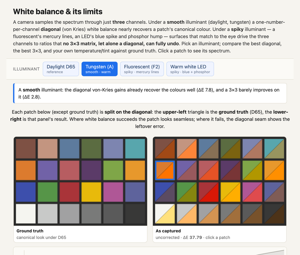 PS1: Image class, point operations, color. Pixel access; brightness and contrast; the luminance–chrominance (YUV) split; gamma; white balance; and the Spanish-Castle afterimage illusion. (→ Chapter 8.1, Image representation, Chapter 8.3, Tone point operations, Chapter 3.2, Perceptual color and trichromatic vision)
 PS2: Convolution and the bilateral filter. Box and Gaussian blur, image gradients, sharpening, and bilateral denoising (with a YUV chroma variant). (→ Chapter 6.2, Convolution, Chapter 10.1, Bilateral filtering)
 PS3: Denoising and demosaicking. Align-and-average a burst (and the ISO/variance story); Bayer demosaicking: basic green, then edge-directed green and color-difference R/B; and Prokudin-Gorsky three-plate color alignment. (→ Part 13, Denoising, Part 15, Demosaicking and joint methods)
 PS4: High dynamic range. Merge an exposure bracket into a radiance map and tone-map it for display. (→ HDR merging, Chapter 18.2, Global tone mapping)
 PS5: Resampling, warping, and morphing. Nearest / bilinear / bicubic / Lanczos resampling; Beier–Neely segment warps; and a full Beier–Neely morph. (→ Chapter 11.1, Warping, Chapter 11.3, Morphing)
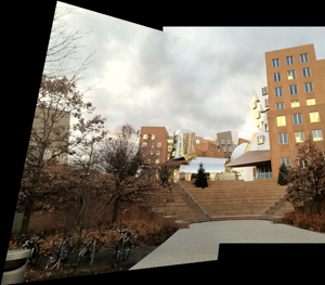 PS6: Homographies and manual panoramas. Homogeneous coordinates, warping by a homography, solving the homography from four point correspondences, and stitching a planar mosaic. (→ Chapter 20.1, Manual panorama stitching from multiple views)
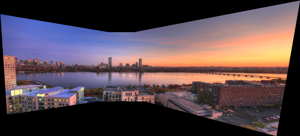 PS7: Automatic panoramas. Harris corners (the structure tensor), patch descriptors, the second-nearest-neighbor ratio test, RANSAC, and feathered / two-scale blending. (→ Chapter 20.2, Automatic panorama stitching from multiple views and feature matching)
 PS8: Non-photorealistic rendering. Paintbrush splatting and single-scale, two-scale, and gradient-oriented painterly rendering. (→ Chapter 25.2, Non-photorealistic rendering)
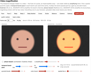 PS9: Make-your-own, video, and ethics. A self-proposed project (optical-flow retiming, phase-based video magnification, and the like) together with the ethics deliverable. Its open menu of advanced topics seeds many sections of Part 33, Computational optics and coded imaging. (→ Chapter 12.8, Optical flow, Chapter 38.3, Motion and video magnification)