BookNotesSlidesP-sets Syllabusdraft · v0.2.49.1
💬Comments welcome. To leave a note, select any text and click the note / highlight button that pops up — or open the panel with the tab at the top-right (‹). Notes are visible only inside our private review group.
Computational Photography, an AI-powered Slopendium — 36 3D and depth
expand to📖 Full book outline1 parts · 10 chapters · 37 sections · 16 figures embedded · 7 placeholders · double-click a figure to enlarge
▸Part 36 3D AND DEPTH⧉
<!--uid: 3d-and-depth-->
▸36.1 Multiple view geometry⧉
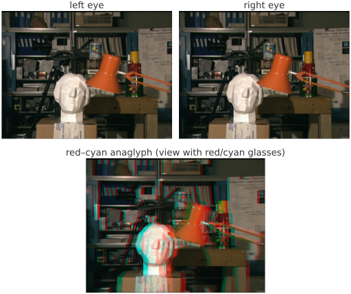
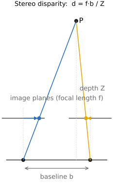
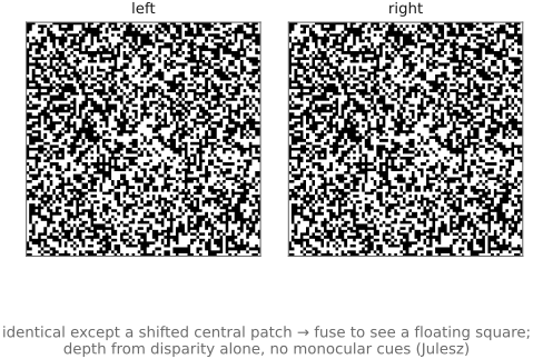
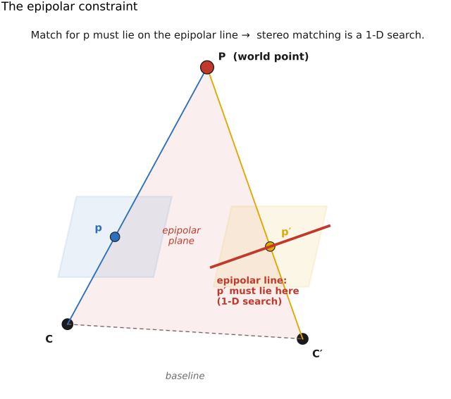
• chapter intro: the leap from one image to **two** — what a second viewpoint buys you (depth), built on the stereo / disparity intuition, then the epipolar-geometry derivation of E/F, with only their estimation and the multi-view scaling-up forwarded
▸36.2 What "depth" means, and where it comes from⧉
• recap, don't re-teach: **depth = the z-coordinate**, *not* the ray length to the point; **unprojection** (pixel + depth → 3-D point) inverts perspective projection (defined in [[Multiple view geometry]] / Fundamentals). A **depth map** is just a per-pixel z image; a **point map** (DUSt3R's term, below) is its unprojected 3-D field.
• the cues/sensors that *give* depth, as a quick inventory (each lives in its home chapter; collected here for contrast):
• **stereo / disparity** — two views, triangulate matched points (baseline + correspondence) → [[Multiple view geometry]]
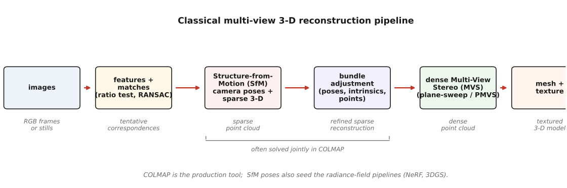
• **multi-view** — many views (the SfM/MVS pipeline below)
• **active depth** — **time-of-flight**, **structured light** (project a known pattern), **LiDAR** — return z directly (pointer to sensors/optics; RealSense & phone face-ID dot projectors)
• **defocus / focus** — depth-from-defocus and focal stacks → [[Computational optics and coded imaging#Light field and multi-aperture imaging]], Depth of field
• **dual-pixel** — the half-aperture parallax phones already capture for autofocus, reused for portrait depth → Optics (dual-pixel AF)
• **motion** — structure-from-motion / optical-flow parallax → [[Matching pixels across space and time]]
• **monocular cues** — a *single* still already implies depth to a human (occlusion, perspective, texture gradient, shading, familiar size, haze); turning those into numbers is the next chapter
• the recurring catch: most reconstructions recover geometry only **up to a similarity** (scale/rotation/translation) unless something fixes the **absolute scale** — a known baseline, a calibration target, or a metric sensor. Keep "relative" vs "metric" depth distinct.
36.2.1 Depth means the camera-frame *z*-coordinate⧉
36.2.2 Depth is the *z*-coordinate, not the ray length⧉
36.2.3 Where depth comes from: a cue-and-sensor inventory⧉
36.2.4 Relative vs metric: the scale you usually don't have⧉
▸36.3 Monocular depth estimation (one image → depth)⧉
⬜ figure not yet created
`fig-monocular-cues` (one photo annotated with each depth cue) fig-monocular-cues
⬜ figure not yet created
`fig-depth-map-relative-vs-metric` (RGB → relative depth → why scale is undetermined without a sensor) fig-depth-map-relative-vs-metric
⬜ figure not yet created
`fig-portrait-bokeh-from-depth` (depth map → depth-graded blur, the phone "portrait mode") fig-portrait-bokeh-from-depth
36.3.1 Why one image cannot determine depth⧉
36.3.2 Relative depth, and the scale-and-shift ambiguity⧉
36.3.3 From hand-built priors to borrowed diffusion priors⧉
36.3.4 What the maps are good for⧉
▸36.4 Single-image 3-D: tour into the picture, photo pop-up, 3-D Ken Burns⧉
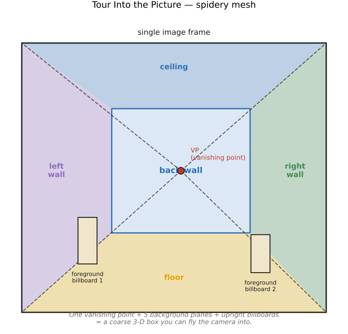
fig-spidery-mesh
fig-spidery-mesh ·
⬜ figure not yet created
`fig-popup-ground-vertical-sky` (geometric-context labels → folded pop-up) fig-popup-ground-vertical-sky
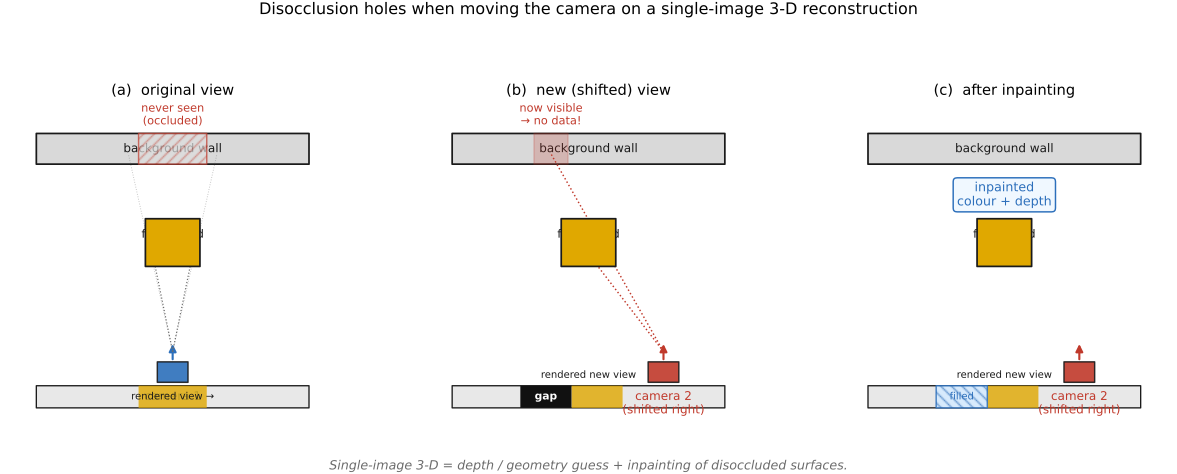
fig-disocclusion-holes
fig-disocclusion-holes ·
36.4.1 The universal recipe, and why holes are the hard part⧉
36.4.2 Tour Into the Picture: the spidery mesh⧉
36.4.3 Automatic Photo Pop-up⧉
36.4.4 3-D Ken Burns and 3-D photos: the monocular form⧉
▸36.5 Multi-view 3-D reconstruction: the classic pipeline⧉
fig-sfm-pipeline
fig-sfm-pipeline ·
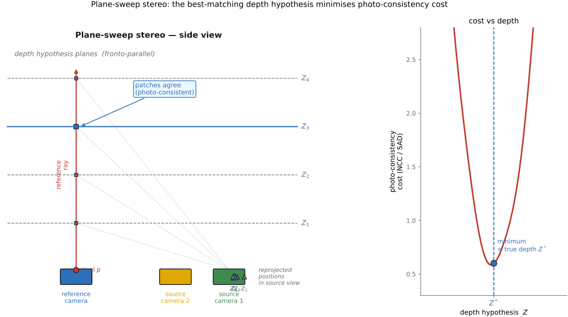
fig-plane-sweep
fig-plane-sweep ·
36.5.1 The pipeline, stage by stage⧉
36.5.2 Why it is brittle — and why SfM survives anyway⧉
▸36.6 Structured light scanning⧉
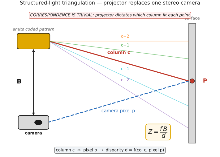
fig-structured-light-triangulation
fig-structured-light-triangulation ·
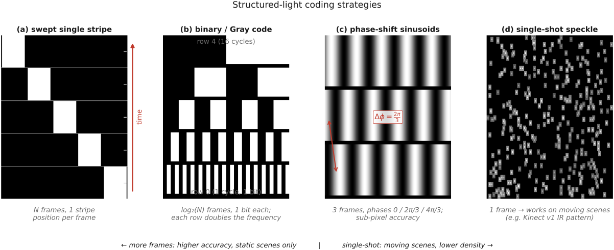
fig-structured-light-codes
fig-structured-light-codes ·
36.6.1 Projector as inverse camera: triangulation with trivial correspondence⧉
36.6.2 The coding ladder, and the frames-versus-motion trade⧉
36.6.3 Calibration and failure modes⧉
▸36.7 Photos → radiance fields and Gaussian splatting (NeRF, 3DGS)⧉
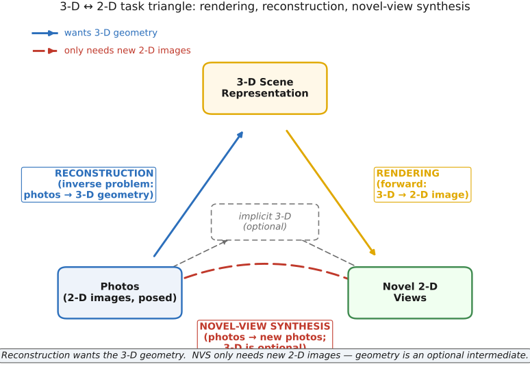
fig-nvs-vs-reconstruction
fig-nvs-vs-reconstruction ·
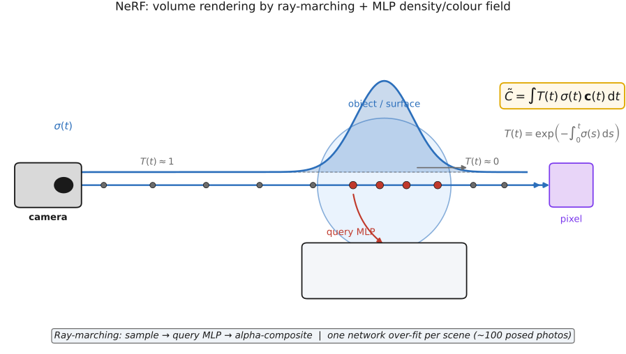
fig-nerf-raymarch
fig-nerf-raymarch ·
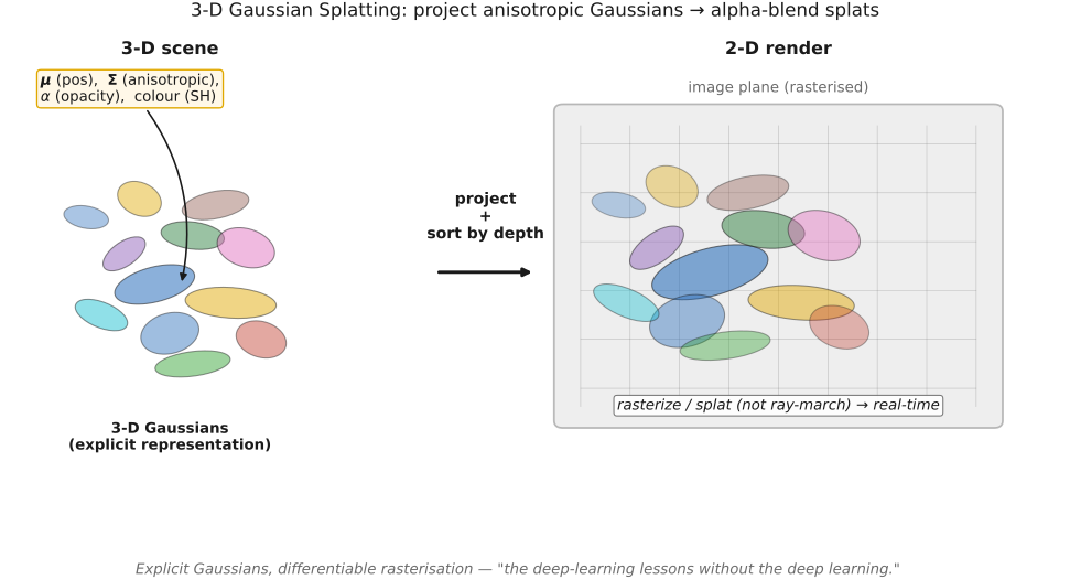
fig-3dgs-splat
fig-3dgs-splat ·
⬜ figure not yet created
`fig-photos-to-splat-pipeline` (capture → COLMAP poses+points → optimize → real-time viewer) fig-photos-to-splat-pipeline
36.7.1 Two goals, one diagram⧉
36.7.2 Inverse differentiable rendering, and the discontinuity that forced fuzziness⧉
36.7.3 NeRF: a scene as a tiny neural network⧉
36.7.4 Do we even need the network?⧉
36.7.5 3-D Gaussian splatting: the lessons without the deep learning⧉
36.7.6 The practical recipe — and what is baked in⧉
36.7.7 Relaxing the assumptions: NeRF in the wild⧉
▸36.8 Feed-forward (amortized) 3-D: skip the per-scene optimization⧉
⬜ figure not yet created
`fig-pointmap` (image + per-pixel depth → unprojected 3-D point field) fig-pointmap
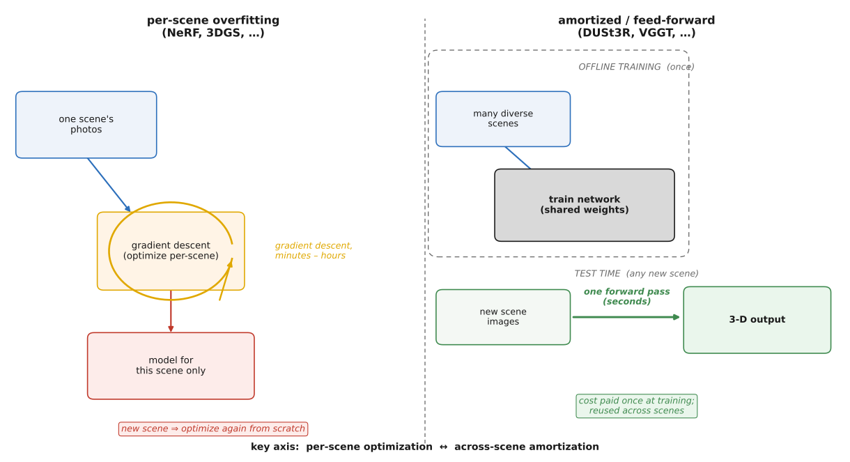
fig-overfit-vs-amortized
fig-overfit-vs-amortized ·
36.8.1 Amortization: pay once, reuse forever⧉
36.8.2 The line: DUSt3R, MASt3R, VGGT⧉
36.8.3 The observation, and the loop it closes⧉
36.8.4 The trade, and the data dependency⧉
▸36.9 Re-photography⧉
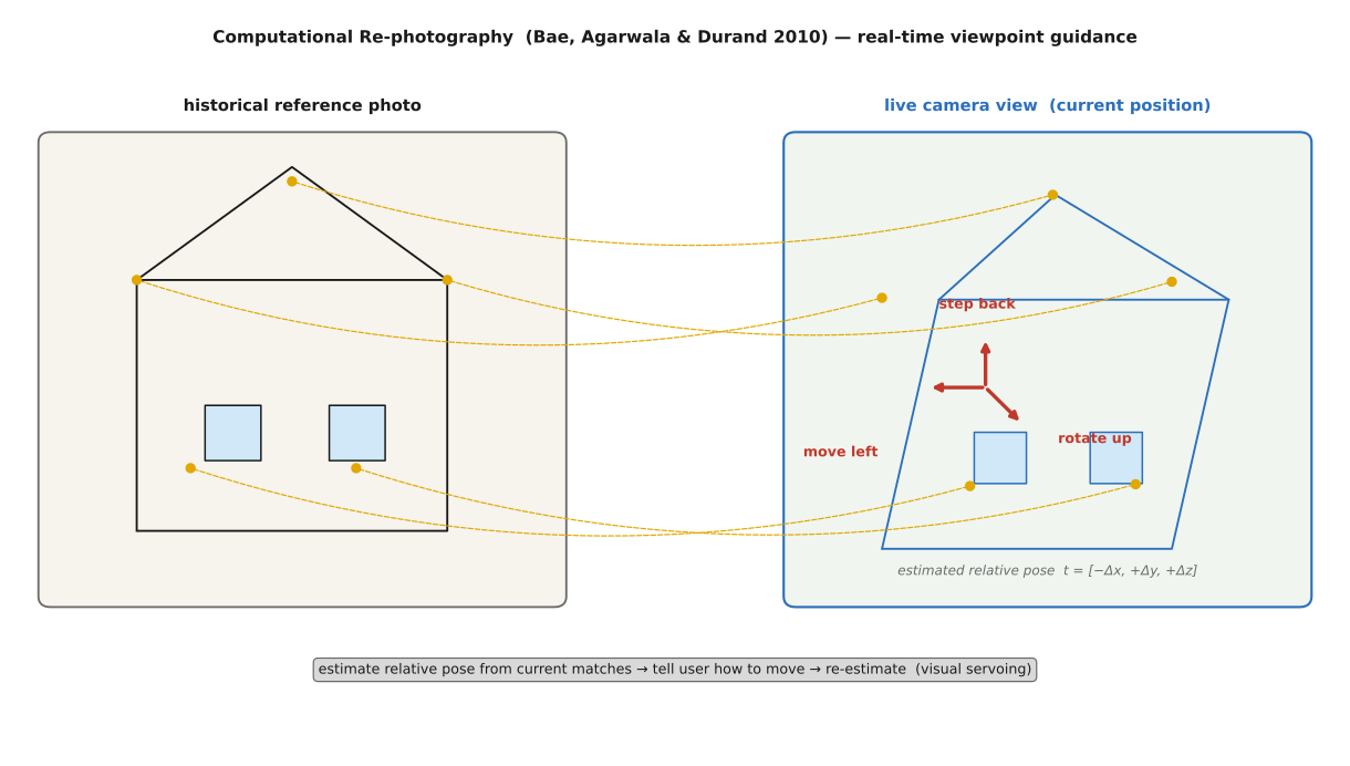
fig-rephotography-guidance
fig-rephotography-guidance ·
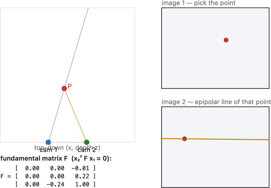
fig-fundamental-matrix
fig-fundamental-matrix · **interactive** epipolar/fundamental-matrix demo (image-pair view, complements the 3-D `fig-epipolar-line`): pick a point in image 1 (u₁,v₁), slide the depth of P along its back-projection ray, and watch P's image slide along the **epipolar line** drawn in image 2; a top-down panel shows the triangulation; camera-2 **baseline + toe-in** sliders change the relative pose; the **fundamental matrix F** (x₂ᵀ F x₁ = 0) is computed live. ✅
36.9.1 Why you cannot just overlay⧉
36.9.2 The real-time guidance loop⧉
36.9.3 Where it sits⧉
▸36.10 The landscape, and is 3-D a "fake task"?⧉
• a deliberately reflective close (slides 84–86): the field is a **complex landscape** along several axes — *reconstruction* (output 3-D) vs *NVS* (output 2-D); *overfit-per-scene* (NeRF, 3DGS) vs *amortized* (DUSt3R, VGGT); *baked illumination* vs *relightable*; **number of input views** (1 → 360° → ∞); the **3-D representation** used (volumetric/fuzzy vs hard surface vs 4-D ray space — or none); how much **prior** is learned; world-space vs camera-space.
• the provocation worth leaving the reader with: the **Bitter Lesson** (Sutton) and the **"parable of the parser"** — when data + compute are plentiful, the hand-built intermediate (here, *explicit 3-D*) may be an unnecessary **"fake task"** that learning can skip. **Is 3-D still needed, or is it scaffolding we'll discard?** (Counterpoint: real applications — robotics, AR, fabrication, autonomous driving — keep wanting *actual* geometry. → [[Adjacent fields and applications]].)
• frontier (slide 50): scalability / long context, beyond shape+texture (materials, **relightability**), **motion** (dynamic scenes), less supervision, fewer inductive biases.
36.10.1 The field spans several design axes⧉
36.10.2 The field as a landscape, not a line⧉
36.10.3 Is 3-D a "fake task"?⧉
36.10.4 The counterpoint, and the frontier⧉