BookNotesSlidesP-sets Syllabusdraft · v0.2.49.1
💬Comments welcome. To leave a note, select any text and click the note / highlight button that pops up — or open the panel with the tab at the top-right (‹). Notes are visible only inside our private review group.
Computational Photography, an AI-powered Slopendium — 12 Matching pixels across space and time
expand to📖 Full book outline1 parts · 11 chapters · 52 sections · 42 figures embedded · 1 placeholders · double-click a figure to enlarge
▸Part 12 MATCHING PIXELS AND HUMANS ACROSS SPACE AND TIME⧉
<!--uid: matching-pixels-and-humans-across-space-and-time-->
💡 **Big lesson (L17 · estimation half):** correspondence-then-transport — this part owns the **hard, ill-posed estimation** half (where did each pixel go?), ill-posed by the **aperture problem** and broken by occlusion and large motion; [[Warping and morphing]] owns the transport. Matching is literally the inverse of warping: warping consumes a coordinate map, matching produces one.
▸12.1 Brute force⧉
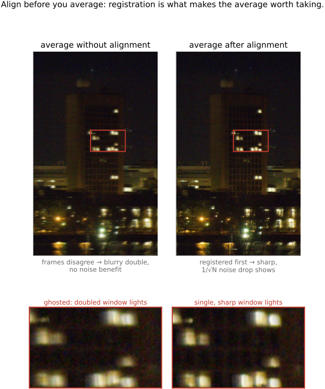
fig-align-before-average
fig-align-before-average · averaging an unregistered hand-held burst (a blurry double) vs averaging the same burst after alignment (sharp, clean, $1/\sqrt N$ benefit visible) ✅
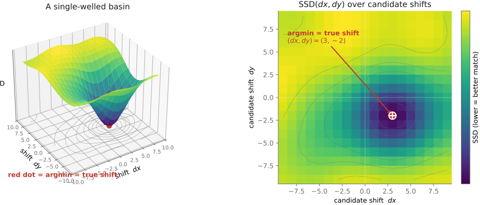
fig-ssd-search-surface
fig-ssd-search-surface · the SSD score over candidate $(dx,dy)$ shifts drawn as a single-welled basin whose minimum marks the true alignment 🟨
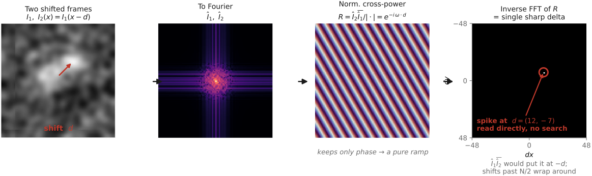
fig-phase-correlation-spike
fig-phase-correlation-spike · two shifted frames producing, via the inverse FFT of the normalized cross-power spectrum, a single sharp delta whose position is the inter-frame shift 🟨
⬜ figure not yet created
L4.8 in a picture)
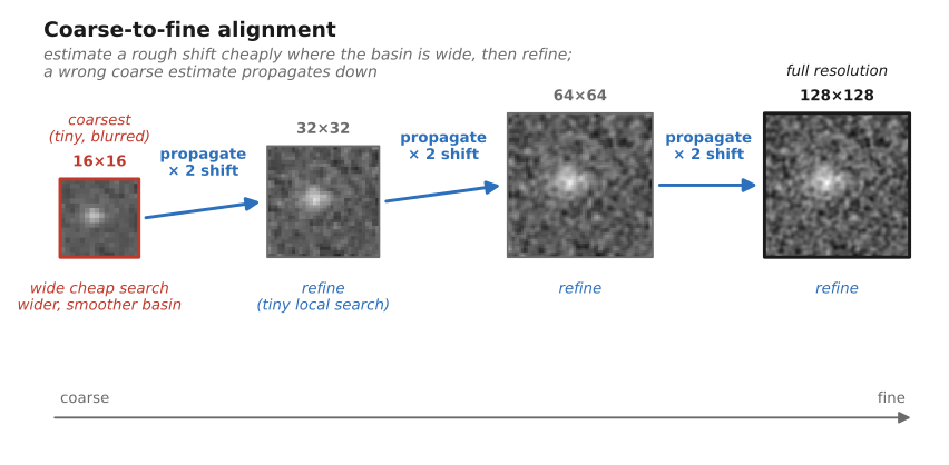
fig-coarse-to-fine-pyramid
fig-coarse-to-fine-pyramid · alignment estimated cheaply at the coarsest pyramid level then propagated and refined down to full resolution, capturing large motions while avoiding local minima 🟨
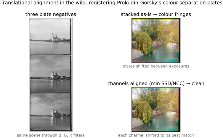
fig-channel-align-sergey
fig-channel-align-sergey · translational alignment in the wild: Prokudin-Gorsky's three color-separation plates stacked naively (color fringes) vs registered by SSD/NCC shift search (clean) ✅
💡 **Big lesson (L4.8 here · diagonalize when you can):** a pure translation is *diagonal* in the Fourier basis — it leaves every magnitude untouched and tilts only the phases by a ramp whose slope **is** the shift. So a brute-force $O(\text{window}^2)$ shift search collapses to a single FFT pair: form the normalized cross-power spectrum, inverse-transform, and read the shift off the location of the resulting delta. Whenever the operator is a shift, a convolution, or a correlation, ask first whether the frequency domain turns the work into a per-frequency (diagonal) operation. *(L4.8, first placed in [[Linearity, Fourier, aliasing and deblurring]]; here it turns a search into a transform.)*
equations
alignment objective $\hat T=\arg\min_T\sum_x(I_1(x)-I_2(Tx))^2$
**SSD** $\sum_{x,y}(I_1(x,y)-I_2(x+dx,y+dy))^2$ (minimized at the true shift
assumes brightness constancy)
**NCC** $\dfrac{\sum(I_1-\bar I_1)(I_2-\bar I_2)}{\sqrt{\sum(I_1-\bar I_1)^2}\sqrt{\sum(I_2-\bar I_2)^2}}$ (maximized toward $+1$
gain/offset-invariant)
**shift theorem** $I_2(x)=I_1(x-d)\Leftrightarrow\hat I_2(\omega)=\hat I_1(\omega)e^{-i\omega\cdot d}$
**normalized cross-power spectrum** $R(\omega)=\hat I_1\overline{\hat I_2}/|\hat I_1\overline{\hat I_2}|=e^{i\omega\cdot d}$ → $\mathcal F^{-1}\{R\}$ is a delta at $d$.
▸12.2 Sub-pixel matching⧉
12.2.1 Refining the cost: fit a parabola⧉
12.2.2 Refining in the frequency domain: phase correlation⧉
12.2.3 Refining by gradient: the Lucas–Kanade step⧉
12.2.4 What breaks it: peak-locking, texture, and noise⧉
12.2.5 One tool, everywhere downstream⧉
▸12.3 Sparse matching⧉
fig-structure-tensor-ellipse
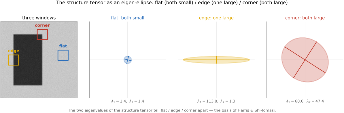
fig-structure-tensor-ellipse · the structure tensor as an eigen-ellipse classifying flat (both eigenvalues small) / edge (one large) / corner (both large) — the basis of Harris & Shi-Tomasi ✅
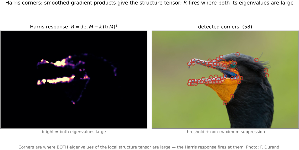
fig-harris-corners
fig-harris-corners · Harris corner detection on a real photo — the structure-tensor response R=det M − k·tr²M, thresholded + non-max-suppressed, corners overlaid (heatmap + detections) ✅
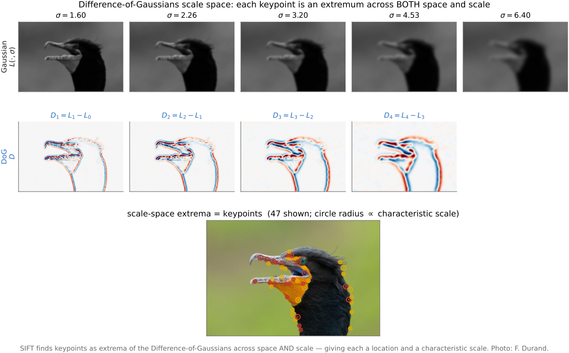
fig-scale-space-dog
fig-scale-space-dog · SIFT keypoint detection — a Gaussian scale space, its Difference-of-Gaussians, and extrema across space AND scale marked with their characteristic scale ✅
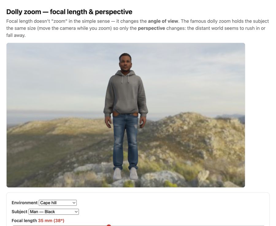
fig-dolly-zoom-sim
fig-dolly-zoom-sim · live dolly-zoom simulator (web edition): hold the subject size while focal length and camera distance trade off so only perspective / background scale changes; log focal (12–200 mm) + distance sliders, realistic Poly Haven environments, subject = head bust or one of six diverse Meshy humans. *Human 3D models generated with Meshy AI.* ✅
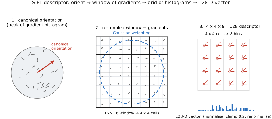
fig-sift-descriptor
fig-sift-descriptor · the $16\times16$ window → $4\times4$ grid of 8-bin orientation histograms → 128-D normalized vector that is the SIFT descriptor 🟨
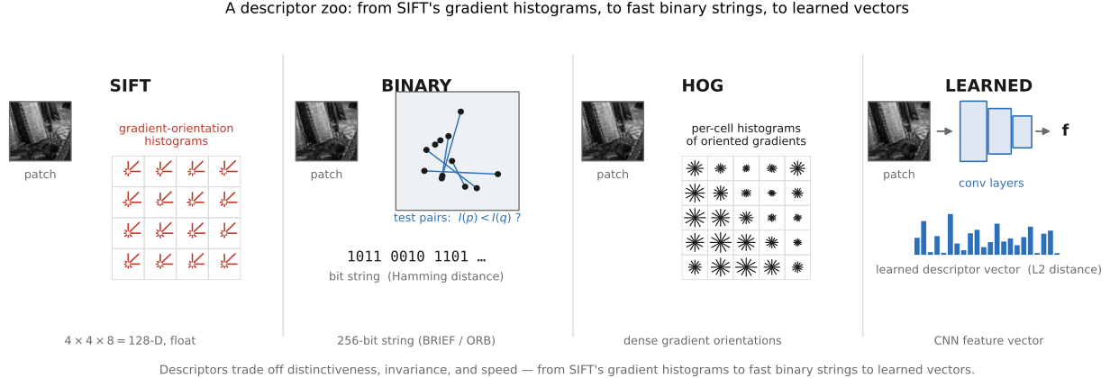
fig-descriptor-zoo
fig-descriptor-zoo · a compact zoo of descriptor families — SIFT gradient-orientation histograms, a binary (BRIEF/ORB) bit-string, HOG-like dense gradients, and a learned CNN vector ✅
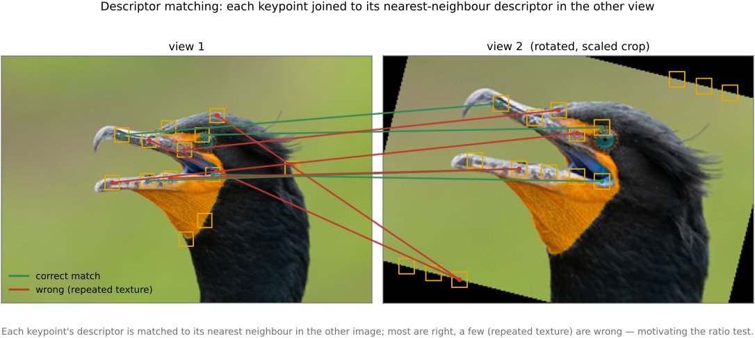
fig-descriptor-matching
fig-descriptor-matching · matching descriptors between two views — keypoints in each, lines joining nearest-descriptor matches, mostly right with a couple of repeated-texture errors (motivates the ratio test) ✅
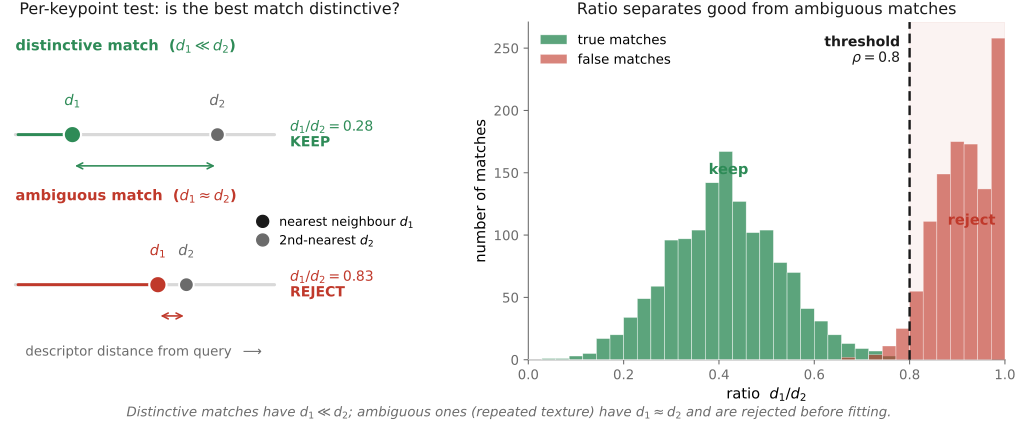
fig-ratio-test
fig-ratio-test · Lowe's ratio test — for one query keypoint, nearest (d1) vs second-nearest (d2) descriptor distances: a distinctive match has d1≪d2 (keep), an ambiguous one d1≈d2 (reject); plus the histogram of d1/d2 for true vs false matches, separated around ρ=0.8 ✅
The previous part transported pixels along maps that were *given* or *hand-drawn*. This part *estimates* the maps, and the cheapest, most robust way to start is not to match every pixel but to match a **sparse** handful of points you can find again. Three stages, in order: **detect** distinctive points (the *where*), **describe** each one's neighborhood (the *what*), and **match** descriptors across images (the *which-goes-with-which*). Detect for **repeatability** (the same physical point fires in both images, despite viewpoint, scale, and lighting), describe for **distinctiveness** (the descriptor is unique enough to match unambiguously and invariant enough to survive the change between images). The raw matches are then filtered — ratio test and RANSAC — in the next section.
💡 **Big lesson (the structure tensor, three jobs):** the same $2\times2$ matrix $M=\sum I\nabla I\nabla I^{\top}$ answers three questions across this part. *Is this a good point to detect?* — yes where $M$ has two large eigenvalues (a corner): **Harris / Shi–Tomasi**, here. *Is this patch's motion solve well-conditioned?* — same matrix invertible: **KLT** ([[Feature tracking]]). *What is the local flow constraint?* — $M$ is the normal-equation matrix $A^\top A$: **Lucas–Kanade** ([[Optical flow]]). Detect with it, track with it, solve flow with it — one matrix, read three ways. Corners are special precisely because the *same* both-directions-vary condition that localizes a point also makes its motion recoverable.
equations
**structure tensor** (second-moment matrix) $M=\sum_{W} w(\mathbf x)\begin{psmallmatrix}I_x^2 & I_xI_y\\ I_xI_y & I_y^2\end{psmallmatrix}$
**Harris response** $R=\det M-k\,(\operatorname{tr}M)^2=\lambda_1\lambda_2-k(\lambda_1+\lambda_2)^2$ (corner if $R$ large, $k\approx0.04$–$0.06$)
**Shi–Tomasi** corner = $\min(\lambda_1,\lambda_2)>\tau$
**scale-space** Difference-of-Gaussian $D(x,y,\sigma)=\big(G_{k\sigma}-G_{\sigma}\big)*I$, keypoint = local extremum in $(x,y,\sigma)$
**SIFT descriptor** = $4\times4$ cells $\times\,8$ orientation bins $=128$-D, $L_2$-normalized
**match** = nearest neighbor by Euclidean distance (float descriptors) or Hamming distance (binary descriptors — ORB/BRIEF).
▸12.4 Feature tracking⧉
fig-track-vs-flow
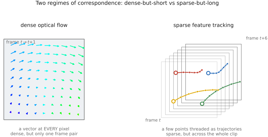
fig-track-vs-flow · two regimes of correspondence — dense flow (one pair, a vector at every pixel; dense but short) vs tracking (a few points threaded as trajectories across many frames; sparse but long) 🟨
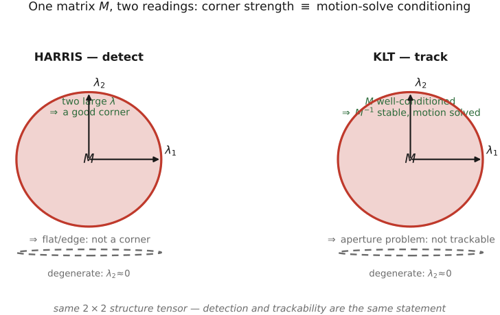
fig-klt-is-harris
fig-klt-is-harris · one matrix, two readings — the same structure-tensor ellipse read as Harris ("good corner to detect?") and as KLT ("motion well-conditioned?"); detection and trackability are the same statement about $M$ 🟨
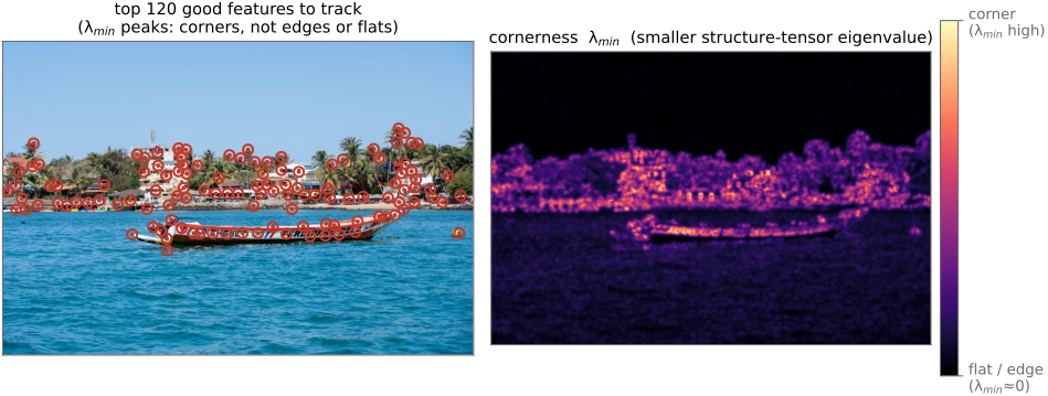
fig-good-features-to-track
fig-good-features-to-track · Shi–Tomasi points land only on corners — markers clustering on corners/junctions, never flat sky or single edges, with windows annotated by their eigenvalue pair; "good feature" = "well-conditioned $M$" = "corner" 🟨
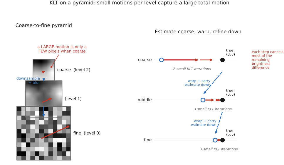
fig-klt-pyramid-iteration
fig-klt-pyramid-iteration · Lucas-Kanade / KLT on a pyramid — a large real motion is a small pixel motion at the coarse level, estimated cheaply then warped and refined down with shrinking residuals ✅
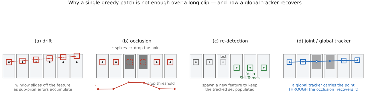
fig-track-drift-occlusion
fig-track-drift-occlusion · three ways a long track fails — drift (window slides off as sub-pixel errors accumulate), occlusion (dissimilarity spikes → drop the feature), re-detection (a fresh Shi–Tomasi point spawned to replace a lost one) 🟨
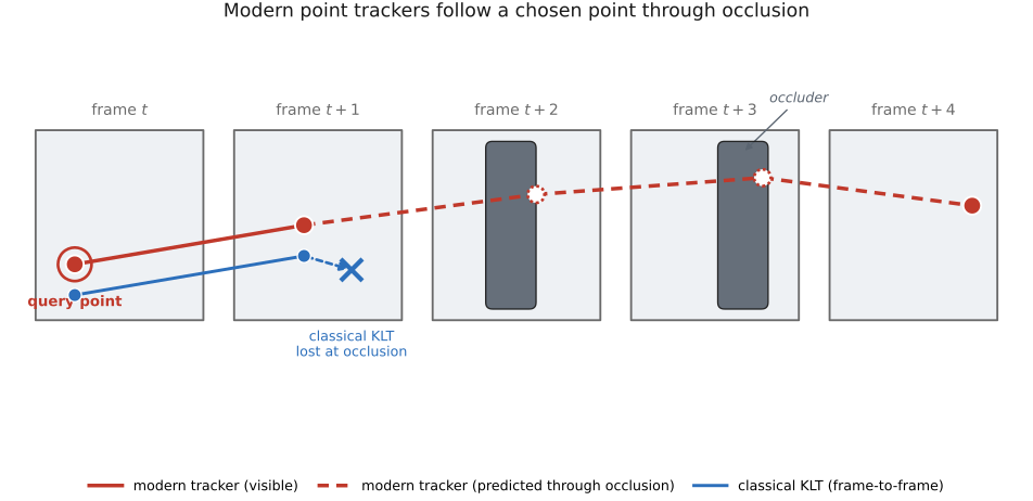
fig-modern-point-trackers
fig-modern-point-trackers · long-range point tracking (TAP/PIPs/CoTracker) — a query point followed across frames as one trajectory, persisting through occlusion (dashed), where classical KLT loses it ✅
The previous section estimated a **dense** flow field — a motion vector at *every* pixel — between *one* pair of frames. This section does the complementary thing: follow a **sparse** handful of *distinctive* points across *many* frames. It is the same physics (brightness constancy, the aperture problem) restricted to the places where the math is well-behaved, and run forward in time. The payoff of the restriction is the chapter's spine: **the matrix that says a patch is a good corner to *detect* is the same matrix that must be invertible to *track* it.** Detect with it (Harris), track with it (KLT), refuse to track where it is singular (Shi–Tomasi). One $2\times2$ matrix, three jobs.
💡 **Big lesson (recurrence of L5.3 — a learned operator swaps a hand-designed prior for one learned from data):** classical KLT tracks a hand-built brightness patch by a hand-derived least-squares update; modern point trackers (PIPs, CoTracker) keep the *exact same task* — "where did this point go?" — but replace the patch with **learned features** and the greedy per-point update with a **learned, occlusion-aware, track-together** module. The skeleton (initialize a trajectory, iteratively refine it against appearance, predict visibility) is unchanged; only the operator is now fit to data. (→ see Big lesson **L5.3**; first appears in [[Deep learning]]. The same "neuralise the classical iteration" move powers RAFT in [[Optical flow]].)
equations
per-feature LK normal equations $M\,\Delta\mathbf{u}=\mathbf{b}$, with the **structure tensor** $M=\sum_{\mathbf{x}\in W} \begin{psmallmatrix}I_x^2 & I_xI_y\\ I_xI_y & I_y^2\end{psmallmatrix}$ and $\mathbf{b}=-\sum_{\mathbf{x}\in W} I_t\begin{psmallmatrix}I_x\\ I_y\end{psmallmatrix}$ → update $\Delta\mathbf{u}=M^{-1}\mathbf{b}$
**Shi–Tomasi trackability** $\min(\lambda_1,\lambda_2)>\lambda_{\min}$ (a feature is trackable iff $M$ is well-conditioned)
affine-warp **dissimilarity** $\varepsilon=\sum_W [\,I_2(A\mathbf{x}+\mathbf{d})-I_1(\mathbf{x})\,]^2$ (occlusion / lost-track test)
12.4.6 An application: synthetic motion blur from a track⧉
▸12.5 Robustness: the ratio test and RANSAC⧉
fig-ratio-test
fig-ratio-test · Lowe's ratio test — for one query keypoint, nearest (d1) vs second-nearest (d2) descriptor distances: a distinctive match has d1≪d2 (keep), an ambiguous one d1≈d2 (reject); plus the histogram of d1/d2 for true vs false matches, separated around ρ=0.8 ✅
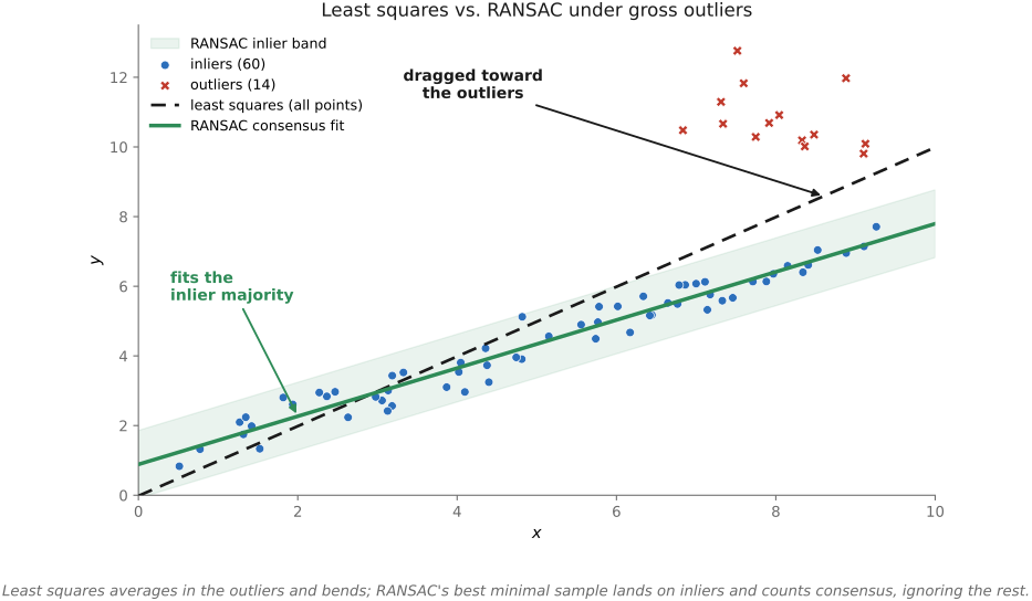
fig-ransac-line-fit
fig-ransac-line-fit · the canonical why-RANSAC picture — points with gross outliers: least squares is dragged off, RANSAC's best minimal-sample line passes through the inlier majority (inlier band shaded) ✅
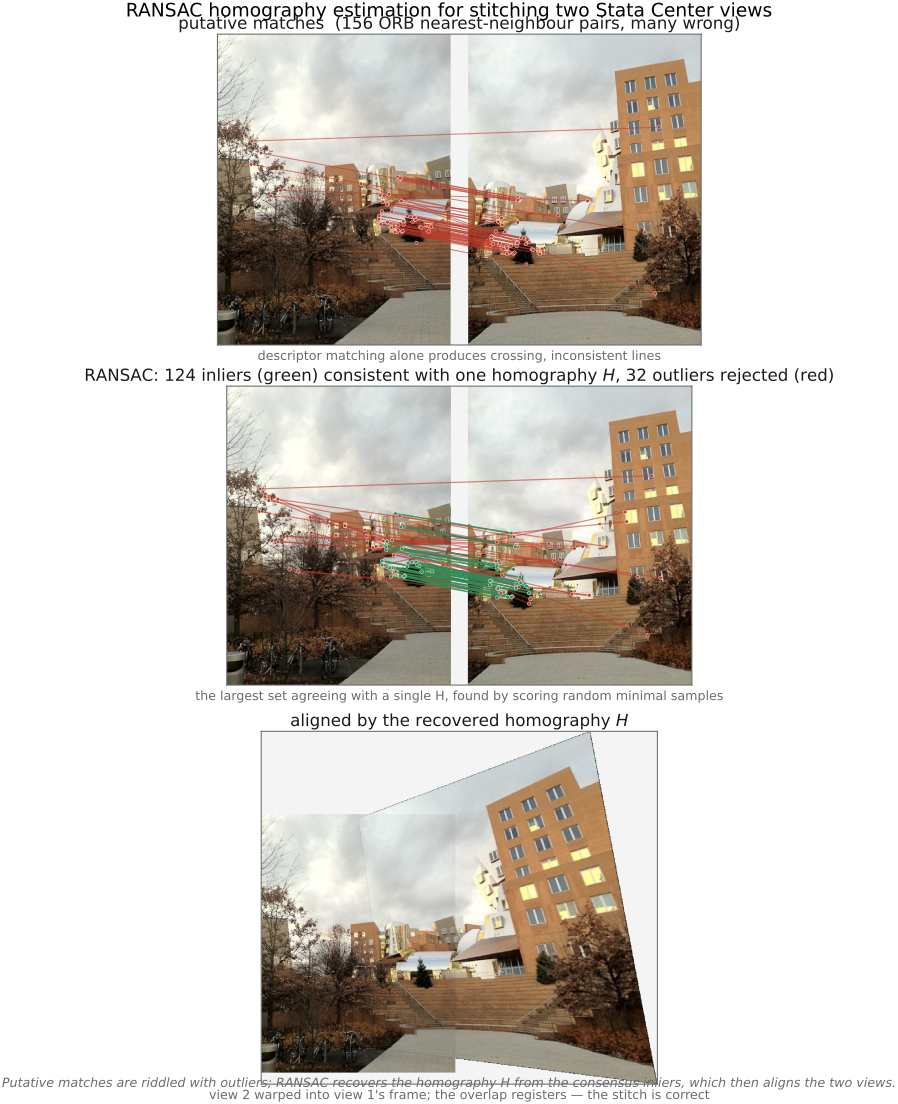
fig-ransac-homography
fig-ransac-homography · two views with raw nearest-neighbor matches (many crossing = wrong) vs the RANSAC inlier set consistent with a single homography (clean, near-parallel) ✅
A keypoint matcher hands you a pile of correspondences that is **mostly noise**: repeated texture, occlusion, and ordinary descriptor collisions all produce confident-but-wrong matches, and a single wrong match wrecks a least-squares fit (one bad point pulls the whole model). Two classic, complementary filters make matching usable — one prunes *before* fitting, the other fits *despite* the survivors' remaining outliers.
equations
**ratio test** accept iff $d_1/d_2<\rho$ (nearest vs second-nearest descriptor distance, $\rho\approx0.7$–$0.8$)
**RANSAC inlier** test $\lVert \mathbf x'_i-T(\mathbf x_i)\rVert<\epsilon$ for the fitted transform $T$
**iteration count** for success probability $p$ with inlier fraction $w$ and minimal-sample size $s$: $N=\dfrac{\log(1-p)}{\log\!\big(1-w^{s}\big)}$ (e.g. $s=4$ for a homography)
keep the $T$ with the most inliers, then **refit** on all inliers (least squares).
▸12.6 Deep learning approaches to sparse matching⧉
fig-learned-feature-pipeline
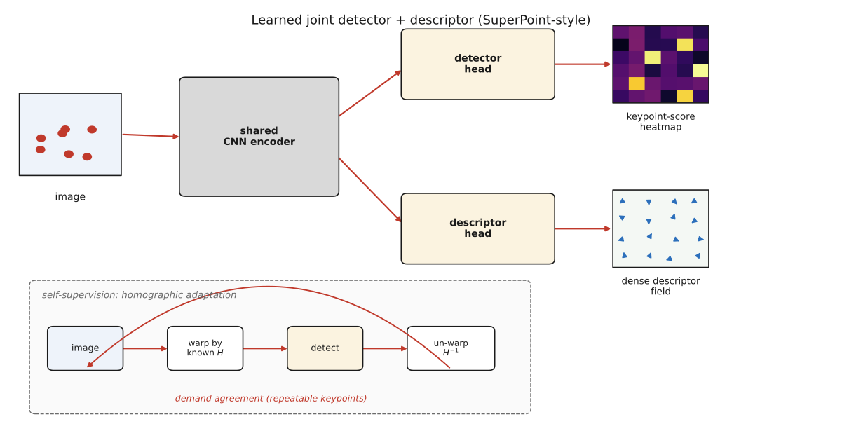
fig-learned-feature-pipeline · SuperPoint-style joint detect-and-describe — a shared CNN encoder splitting into a detector head (keypoint heatmap) and a descriptor head (dense field), with a homographic-adaptation self-supervision inset ✅
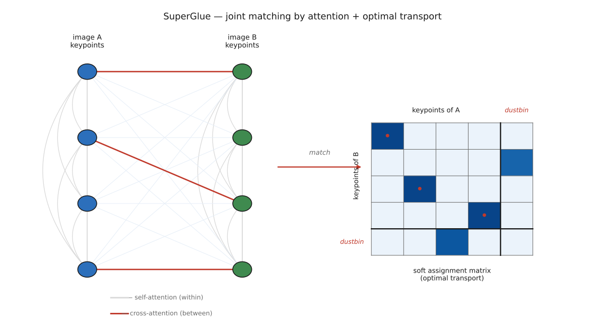
fig-superglue-attention
fig-superglue-attention · SuperGlue — two keypoint sets as graph nodes, self- and cross-attention edges, and a soft optimal-transport assignment matrix with a dustbin row/column for unmatched points ✅
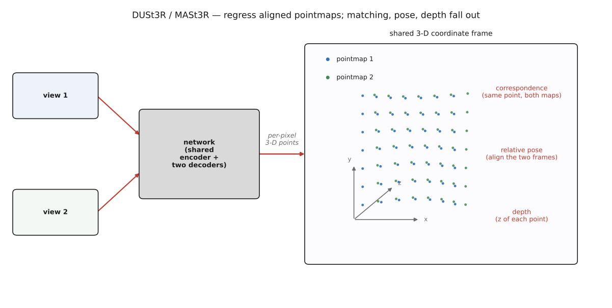
fig-dust3r-pointmap
fig-dust3r-pointmap · DUSt3R/MASt3R — an image pair regressed into two dense pointmaps in one common frame, so correspondence, relative pose, and depth read off the aligned points (no keypoint stage) ✅
The classical pipeline — hand-designed detector, descriptor, nearest-neighbor matcher — is exactly the kind of three-stage hand-built system deep learning likes to swallow whole (the **L5.3** move: learn the operator from data). It arrives in three waves. First, **learned local features** that play SIFT's role — joint detector-and-descriptor networks (**LIFT**, **SuperPoint**, **D2-Net**, **R2D2**) trained for repeatability and matchability, often **self-supervised** by warping an image with known homographies and demanding consistent keypoints. Second, **learned matching** that reasons about the *whole set* of features at once instead of independent nearest-neighbors: **SuperGlue** (and the faster **LightGlue**) cast matching as graph/attention-based assignment (an optimal-transport-flavoured solve), while **detector-free** matchers like **LoFTR** skip keypoints entirely and match dense coarse-to-fine. Third, the **3-D-aware** turn — **DUSt3R / MASt3R** regress dense **pointmaps** directly from an image pair, so correspondence, camera pose, and depth fall out together with no explicit keypoint stage at all; matching stops being a separate step and becomes a by-product of predicting geometry. Each wave keeps the *task* and learns more of the *pipeline*.
equations
SuperGlue's matching as an **optimal-transport** assignment — maximize $\sum_{i,j}P_{ij}S_{ij}$ over (doubly-stochastic, dustbin-augmented) $P$ via Sinkhorn, $S$ the learned score matrix
contrast the classical per-point $\arg\min_j\lVert d_i-d_j\rVert$.
▸12.7 Fast matching⧉
fig-ann-tradeoff
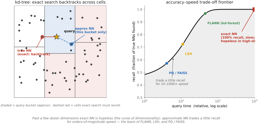
fig-ann-tradeoff · approximate nearest neighbor — exact kd-tree backtracking vs an approximate bucket lookup, beside a recall-vs-query-time frontier (exact, FLANN, LSH, PQ/FAISS) ✅
fig-dolly-zoom-sim
fig-dolly-zoom-sim · live dolly-zoom simulator (web edition): hold the subject size while focal length and camera distance trade off so only perspective / background scale changes; log focal (12–200 mm) + distance sliders, realistic Poly Haven environments, subject = head bust or one of six diverse Meshy humans. *Human 3D models generated with Meshy AI.* ✅
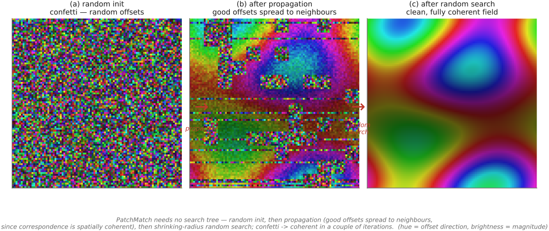
fig-patchmatch-propagation
fig-patchmatch-propagation · PatchMatch's three steps on a nearest-neighbor field shown as a color image — random init (confetti) → propagation (coherent regions snap in) → random search (clean) ✅
Once you have descriptors, the cost is dominated not by computing them but by the **nearest-neighbor search** in a high-dimensional space — and exact NN is hopeless at scale (the curse of dimensionality defeats kd-trees past a few dozen dimensions). So the toolkit is **approximate** NN and clever propagation. For sparse descriptors: randomized **kd-trees / FLANN**, **locality-sensitive hashing** (collide nearby points into the same bucket), and **product quantization** for billion-scale retrieval (the lineage that became FAISS / ScaNN vector databases). For *dense* patch correspondence, **PatchMatch** abandons search trees entirely — random initialization plus **propagation** (good matches are spatially coherent, so a neighbor's offset is a great guess) plus occasional random refinement converges astonishingly fast ([[Patch match]]). Worth singling out is **Andrew Adams's random-projection lineage** — Gaussian kd-trees and the **permutohedral lattice** — which finds good high-dimensional matches by projecting onto a few random directions and splatting/propagating on a lattice; the same machinery accelerates the bilateral filter and NL-means denoising ([[Slopendium/Denoising]]). The recurring lesson: at scale, *good-enough-and-fast* beats *optimal-and-slow*, and **propagation** (exploit coherence) often beats **search** (treat each query independently).
▸12.8 Optical flow⧉
fig-flow-field-colorkey
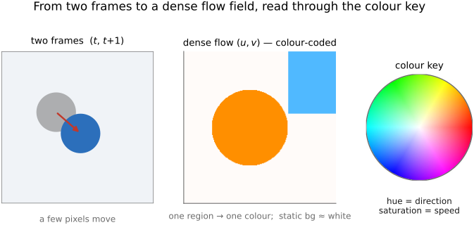
fig-flow-field-colorkey · from two frames to a dense field — a per-pixel flow shown with the standard color key (hue = direction, saturation = speed, after Baker et al. 2011); coherent regions read as one color, static background near-white ✅
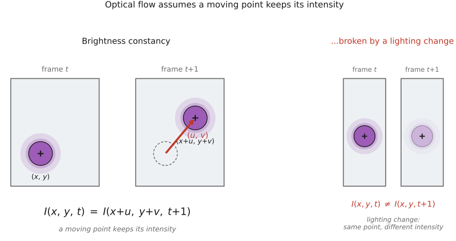
fig-brightness-constancy
fig-brightness-constancy · the assumption $I(x,y,t)=I(x+u,y+v,t{+}1)$ and where it breaks — three insets failing it (a surface re-lit, a sliding specular highlight, an occlusion with no counterpart) ⬜
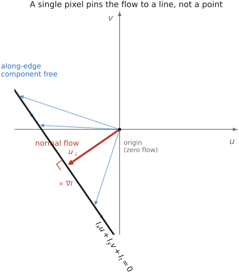
fig-flow-constraint-line
fig-flow-constraint-line · one equation, a line of answers — $I_x u + I_y v + I_t = 0$ as a line in the $(u,v)$ plane; the gradient fixes only the normal component (normal flow), the along-edge tangent undetermined 🟨
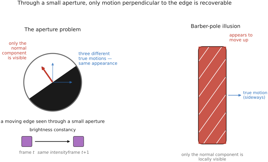
fig-aperture-problem
fig-aperture-problem · why one pixel is not enough — a straight edge through an aperture (three true motions, identical appearance, only normal recoverable) and the barber-pole illusion (diagonal stripes appearing to move straight up) 🟨
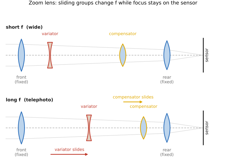
fig-zoom-mechanism
fig-zoom-mechanism · a zoom at two focal lengths (short-f/wide vs long-f/tele): moving variator + compensator groups slide along the axis to change f while the focal plane (sensor) stays fixed; motion arrows between states ✅
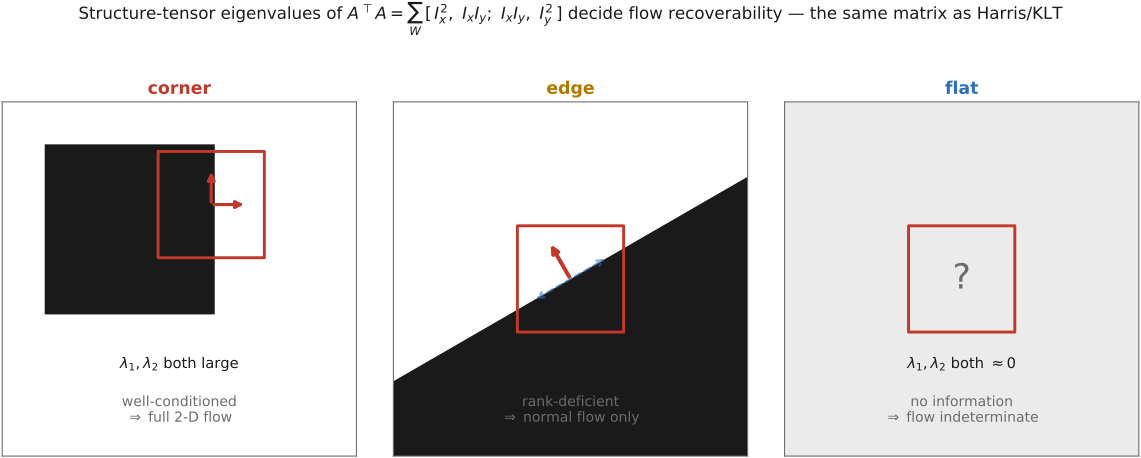
fig-flow-corner-edge-flat
fig-flow-corner-edge-flat · the structure tensor $A^\top A$ deciding where flow is solvable — corner (two large eigenvalues, full 2-D flow), edge (rank-deficient, only normal flow), flat (indeterminate); the same picture that selected Harris corners 🟨
fig-klt-pyramid-iteration
fig-klt-pyramid-iteration · per-feature coarse-to-fine LK — for one patch, solve the $2\times2$ system at a blurred level, warp, recompute $I_t$, re-solve for a residual, propagate down; LK localized to a single window run down the pyramid ⬜
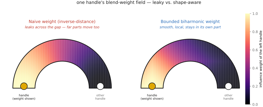
fig-bbw-weights
fig-bbw-weights · one handle's blend-weight field on a 2-D limbed shape: naive inverse-distance weight LEAKS across the gap to far parts, vs. bounded biharmonic weight that is smooth, local, non-negative and stays in its own part (magma heat-maps) ✅
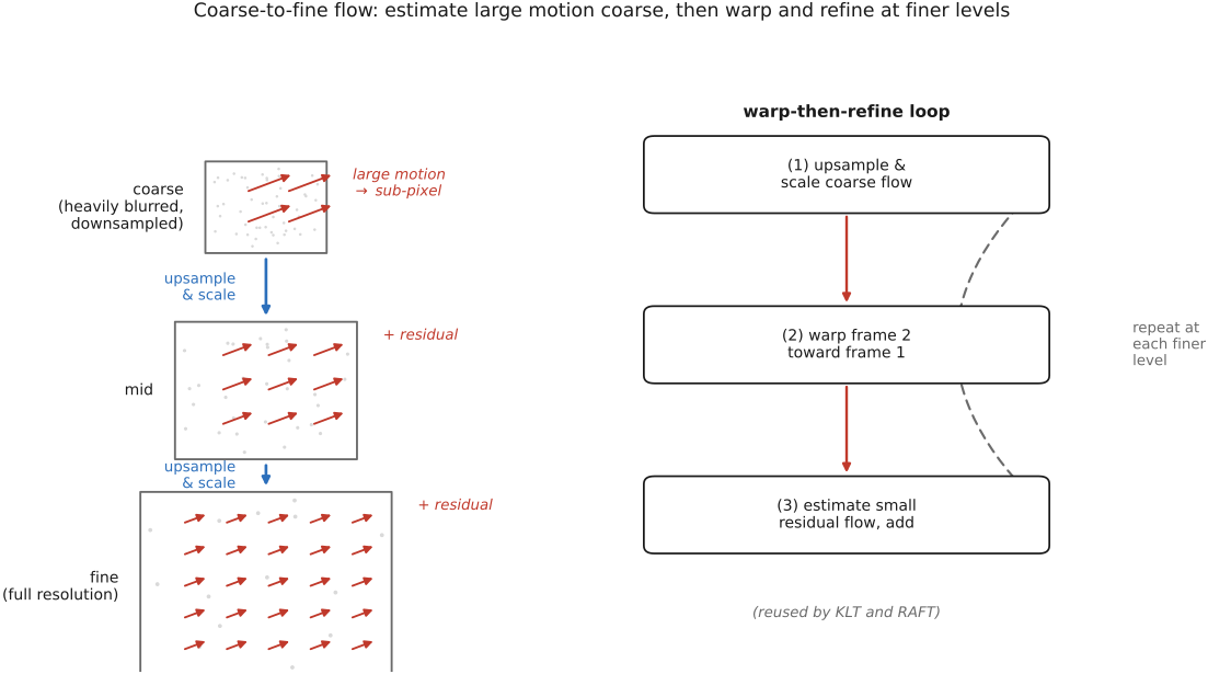
fig-coarse-to-fine-flow
fig-coarse-to-fine-flow · making large motion sub-pixel — a Gaussian pyramid where coarse displacement is fractional; at each level upsample-and-scale, warp, estimate the small residual and add; a Laplacian view of the flow 🟨
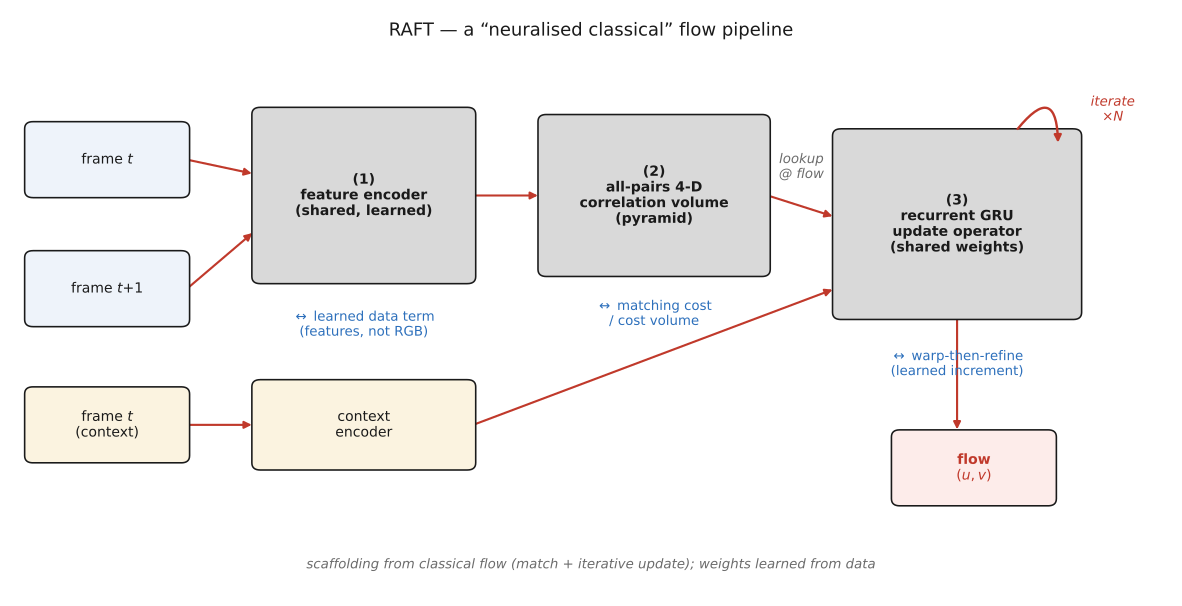
fig-raft-skeleton
fig-raft-skeleton · RAFT, the classical pipeline neuralized — learned feature + context encoders, an all-pairs 4-D correlation volume, and a recurrent GRU update operator iterating; the boxes line up with data term, cost volume, and warp-then-refine 🟨
💡 **Big lesson (the chapter's core — *brightness constancy + the aperture problem*):** track a point by the one thing that's (assumed) conserved — its **brightness**. Linearizing that single scalar equation gives **one constraint per pixel**, $I_x u + I_y v + I_t = 0$, for **two** unknowns $(u,v)$ — so locally motion is **fundamentally underdetermined**: you can only see the component **along the image gradient** (normal flow), never the component **along an edge** (the *aperture problem*). Every flow method is a strategy for supplying the missing second equation — from a **neighbor** (Lucas–Kanade: pixels in a patch share a motion → the well-/ill-posedness is the **same corner/edge/flat structure tensor as Harris**), from a **smoothness prior** (Horn–Schunck), or from **learned context** (RAFT). *Only the gradient carries motion information, and one gradient is never enough.*
▸12.9 Deep learning approaches to optical flow⧉
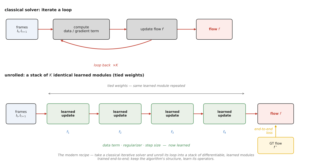
fig-flow-unrolling
fig-flow-unrolling · the unrolling pattern — a classical iterative solver's loop (data term → update → repeat) beside its unrolled stack of identical learned modules (tied weights) trained end-to-end ✅
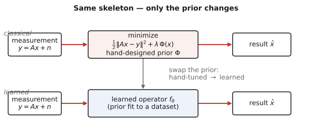
fig-learned-vs-handdesigned
fig-learned-vs-handdesigned · same inverse-problem skeleton, prior swapped: classical (data-fit + hand prior $\Phi$) vs learned ($f_\theta$ fit to data) (ML) ✅
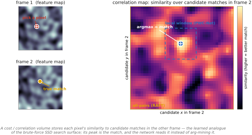
fig-cost-volume
fig-cost-volume · the correlation/cost volume (learned analog of the SSD search surface) — a pixel's similarity to candidate matches in the other frame, a heatmap whose argmax is the match (local PWC-Net vs all-pairs RAFT) ✅
fig-raft-skeleton
fig-raft-skeleton · RAFT, the classical pipeline neuralized — learned feature + context encoders, an all-pairs 4-D correlation volume, and a recurrent GRU update operator iterating; the boxes line up with data term, cost volume, and warp-then-refine 🟨
The learned-flow story is best told as a single pattern rather than a parade of networks: **take the classical iteration of [[Optical flow]] and *unroll* it into a differentiable network trained end-to-end**, so the hand-tuned data term, smoothness regularizer, and coarse-to-fine schedule become learned. **FlowNet** first showed a CNN could regress dense flow at all. **PWC-Net** made the lineage explicit by folding the *classical* pipeline — **P**yramid, **W**arping, **C**ost-volume — into a compact, fast network: the same coarse-to-fine warping of the previous section, now with learned features and a learned update. **RAFT** is the design that came to dominate — build a 4-D **all-pairs correlation volume** (every pixel's similarity to every other) and apply a **recurrent update operator** that behaves like an unrolled iterative optimizer refining the field; it is the flow analog of "neuralize the classical solver" and the reason RAFT-style modules now appear in stereo, scene flow, and tracking. Transformer flows (**FlowFormer**, **GMFlow**) reframe the same problem as **global matching**, replacing the local cost-volume update with attention. Throughout, the *skeleton* — features, a cost/correlation volume, an iterative update, coarse-to-fine — is the classical one; learning supplies the operators.
equations
the unrolling view — classical $\
\mathbf f^{(k+1)}=\mathbf f^{(k)}-\eta\,\nabla E(\mathbf f^{(k)})\
$ becomes $\
\mathbf f^{(k+1)}=\mathbf f^{(k)}+\text{GRU}_\theta\big(\mathbf f^{(k)},\,\text{corr lookup}\big)$, the learned update standing in for the gradient step.
▸12.10 Face tracking⧉
12.10.1 Detecting the face⧉
12.10.2 Landmarks: pinning down the features⧉
12.10.3 Tracking across time⧉
12.10.4 Lifting to 3-D: the morphable model⧉
12.10.5 Recognition, and the dark side⧉
12.10.6 Which library to use⧉
▸12.11 Body pose estimation⧉
12.11.2 On-device, real time⧉
12.11.3 Lifting to 3-D: parametric bodies⧉
12.11.4 Which library to use⧉