BookNotesSlidesP-sets Syllabusdraft · v0.2.49.1
💬Comments welcome. To leave a note, select any text and click the note / highlight button that pops up — or open the panel with the tab at the top-right (‹). Notes are visible only inside our private review group.
Computational Photography, an AI-powered Slopendium — 08 Basic image processing and ISP
expand to📖 Full book outline1 parts · 13 chapters · 84 sections · 32 figures embedded · 8 placeholders · double-click a figure to enlarge
▸Part 8 BASIC IMAGE PROCESSING AND ISP⧉
<!--uid: basic-image-processing-and-isp-->
At the end of this part, the readers will be able to implement a complete ISP or very basic version of a photo editing software (mini lightroom) with exposure, contrast, etc.
▸8.1 Image representation⧉
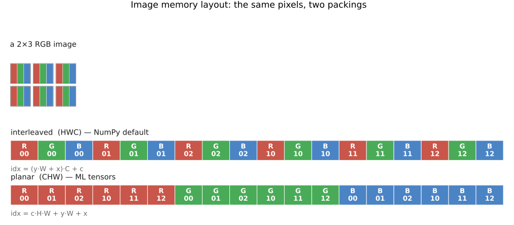
fig-image-memory-layout
fig-image-memory-layout · a 2×3 RGB image packed into 1-D memory two ways — interleaved HWC (NumPy) vs planar CHW (ML), with the stride formulas (Image representation, BASIC) 🟨
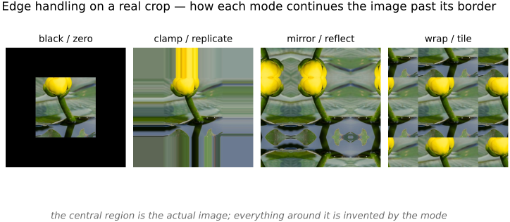
fig-edge-handling-photo
fig-edge-handling-photo · the four edge modes on a real crop — black / clamp / mirror / wrap continued past the border; real-image companion to `fig-edge-handling` (Image representation → falling off the edge, BASIC) ✅
8.1.13 Pixel lookups and boundaries⧉
▸8.2 What the numbers mean⧉
8.2.1 What the numbers actually mean: encoding⧉
8.2.2 What the numbers actually mean: color spaces⧉
▸8.3 Tone point operations⧉
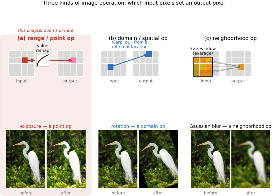
fig-operation-types
fig-operation-types · the three image-operation types — range (point) vs domain (spatial) vs neighborhood (Values / point ops, BASIC) 🟨
8.3.9 Converting to black and white⧉
▸8.4 Beauty curves: the camera "look"⧉
8.4.7 Vignetting and grain, added on purpose⧉
8.4.8 Our curve, in code⧉
8.4.10 Beauty curves in real ISPs⧉
▸8.5 Color point operations⧉
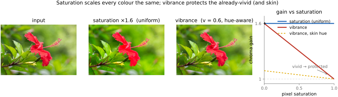
8.5.1 Basic color enhancement: saturation and vibrance⧉
8.5.2 The color edits, in code⧉
8.5.3 Converting to black and white⧉
8.5.4 Video color grading⧉
▸8.6 Color beautification and preferred colors⧉
⬜ figure not yet created
`fig-color-look-corridors` (interactive, requested below) fig-color-look-corridors
⬜ figure not yet created
hue-vs-hue plot of translation vs contraction
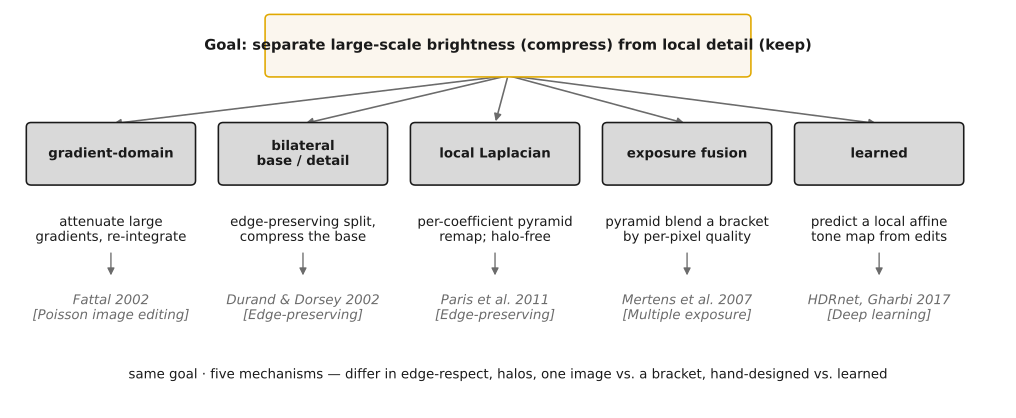
fig-tonemap-taxonomy
fig-tonemap-taxonomy · a taxonomy of local tone mapping — bilateral base/detail, gradient-domain, local Laplacian, exposure fusion, learned — placed on a shared axis 🟨
⬜ figure not yet created
before/after sky and skin crops fig-wb-before-after
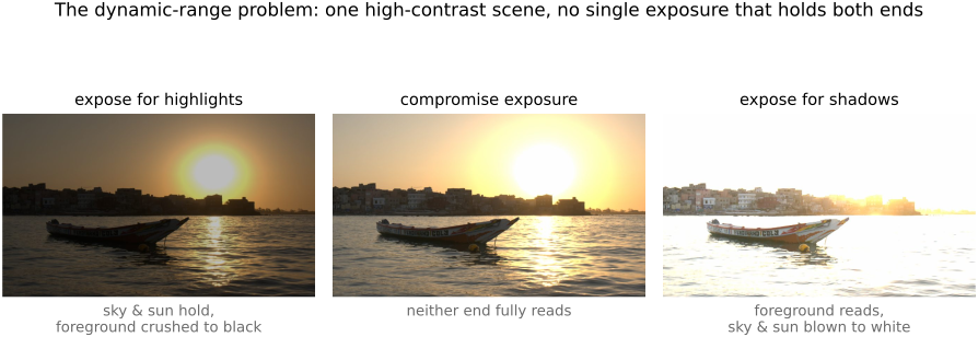
fig-dynamic-range-problem
fig-dynamic-range-problem · the dynamic-range problem on a real HDR photo: one sunset-over-river capture developed at three exposures — expose for highlights (foreground crushed) / compromise / expose for shadows (sky blown) — no single exposure holds both ends (BASIC tone mapping) ✅
▸8.7 Histograms⧉
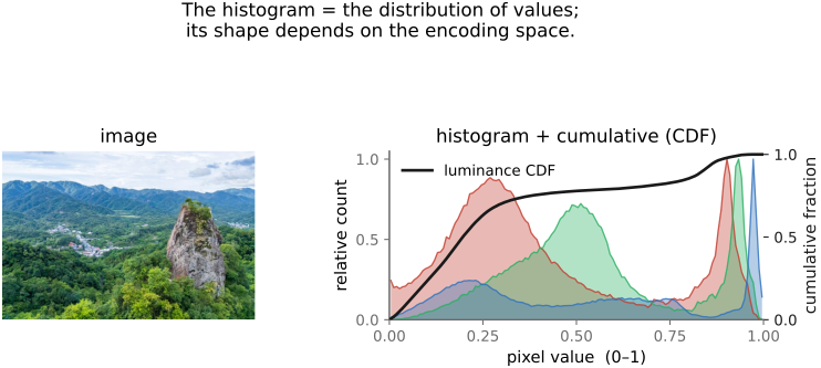
fig-histogram
fig-histogram · an image histogram (per-channel) + cumulative histogram; its shape depends on the encoding space (BASIC tone mapping) 🟨
fig-histogram-encoding-spaces
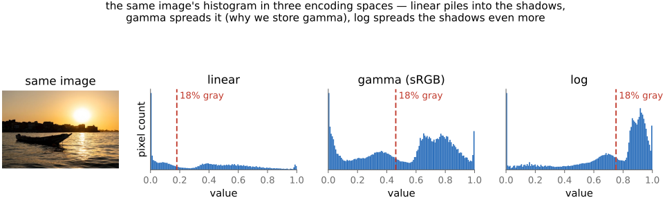
fig-histogram-encoding-spaces · the same image's luminance histogram in linear / gamma (sRGB) / log; 18% gray marked at 0.18 / ~0.46 / ~0.75 — the encoding reshapes the value axis (BASIC histograms) 🟩
fig-histogram-equalization
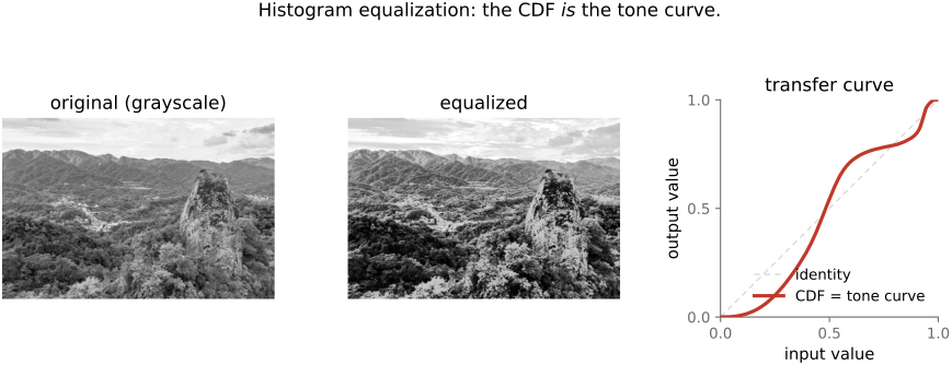
fig-histogram-equalization · histogram equalization — the CDF used as the transfer curve, before/after (BASIC) 🟨
fig-histogram-matching
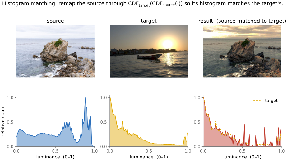
fig-histogram-matching · histogram matching — source + target images and their histograms → matched result, with the composed transfer curve $\text{CDF}_\text{tgt}^{-1}\circ\text{CDF}_\text{src}$ (BASIC histograms) ✅
• the **histogram** — the distribution of pixel values — is the natural companion to point operations: this short chapter is how to *read* it, and how it can *drive* an automatic tone curve
▸8.8 Sharpening⧉
fig-unsharp-mask
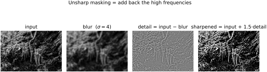
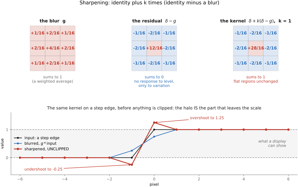
fig-unsharp-mask · unsharp-mask decomposition: input − blur = detail (high-pass), output = input + k·detail 🟨
fig-sharpen-kernel
fig-sharpen-kernel · the sharpening kernel δ − blur as a +center / −surround stencil 🟨
▸8.9 Dead pixels⧉
fig-operation-types
fig-operation-types · the three image-operation types — range (point) vs domain (spatial) vs neighborhood (Values / point ops, BASIC) 🟨
fig-ssim-map
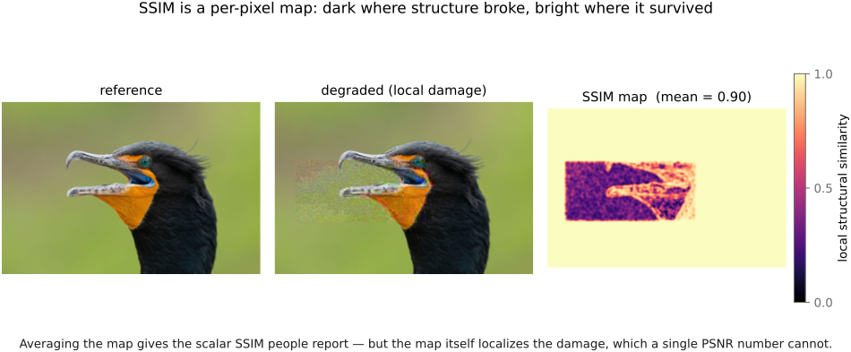
fig-ssim-map · SSIM as a per-pixel map: reference, locally-damaged copy (one band JPEG-blocked + noised), and the SSIM heat-map that goes dark exactly on the damage — its mean is the scalar SSIM (Image metrics, BASIC) ✅
fig-color-space-atlas
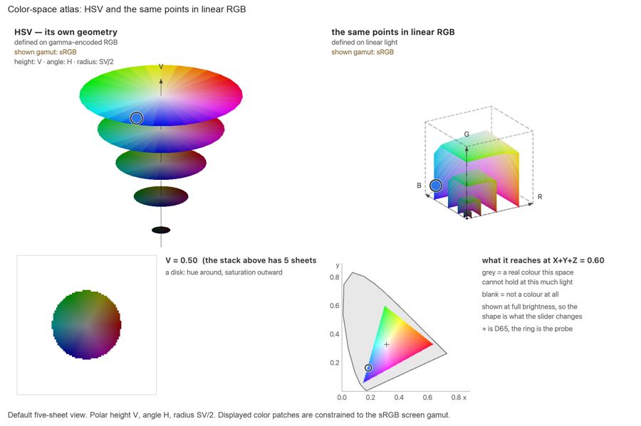
fig-color-space-atlas · **interactive** color-space atlas: one space drawn twice, in its own geometry (cube / cone / bi-cone / warped cube) and in a chosen ambient frame (XYZ, LMS, linear RGB, sRGB, Chong, Oklab), from the same lattice, as edges / voxels / one slice; MacAdam ellipses optional; click to read coordinates in both; stripes for colors outside sRGB. Placed at the end of the perceptually-uniform section of **4.6 Advanced color**, where it works as the chapter's capstone: by then HSV/HSL, CIELAB, Oklab and Chong have each been shown alone, and the atlas is about the map between them. URL carries the state (`?space=&ambient=&mode=&axis=&at=&grid=&macadam=&zebra=`). 🟨
⬜ figure not yet created
the star-eater failure.
• dead / stuck / hot pixels — what each reports, and why hot pixels grow with exposure time, heat, and ISO
• where they come from: manufacturing defects vs aging; dark current doubling every 6–8 °C
• finding them: factory defect map (ships in-camera / travels as DNG FixBadPixels) + dark-frame calibration (long-exposure NR, pixel mapping)
• fixing them: concealment by same-color interpolation, before demosaicking; the star-eater pitfall of over-aggressive suppression
8.9.1 Where they come from⧉
8.9.2 Finding them⧉
8.9.3 Fixing them⧉
▸8.10 Auto-exposure and auto white balance⧉
fig-ae-metering
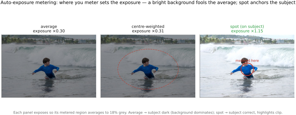
fig-ae-metering · **interactive** AE metering modes: pick a scene + mode (average / center-weighted / movable+resizable spot); the demo exposes so the metered region averages 18% and reports metered tone, gain, and clipped %; "where you meter sets the exposure" ✅
fig-white-balance-real
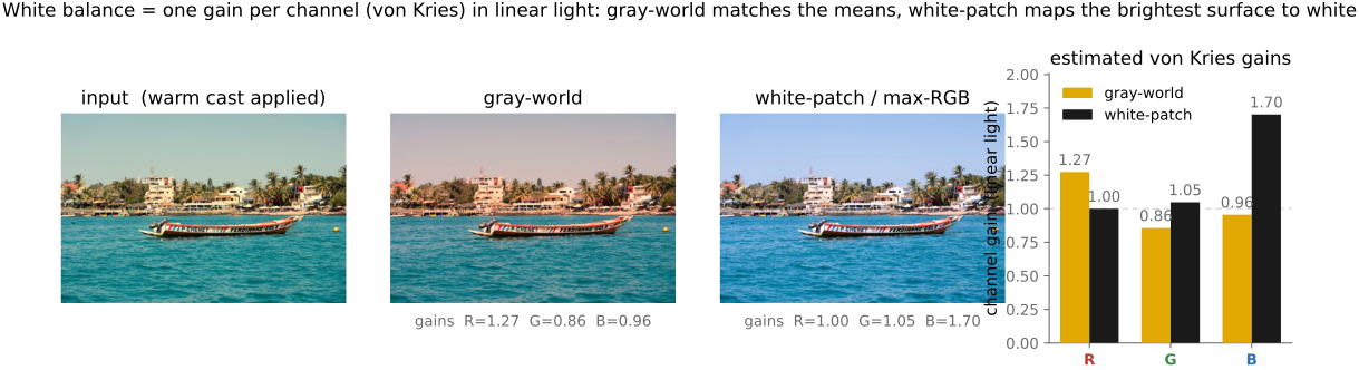
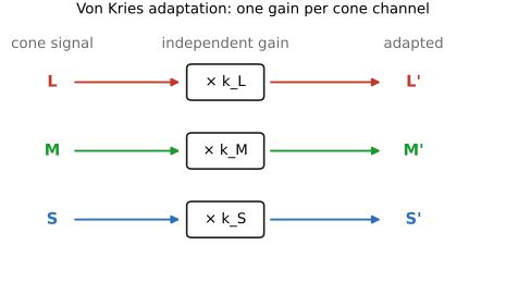
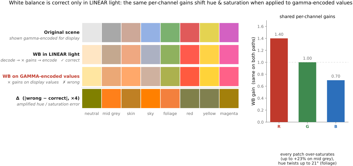
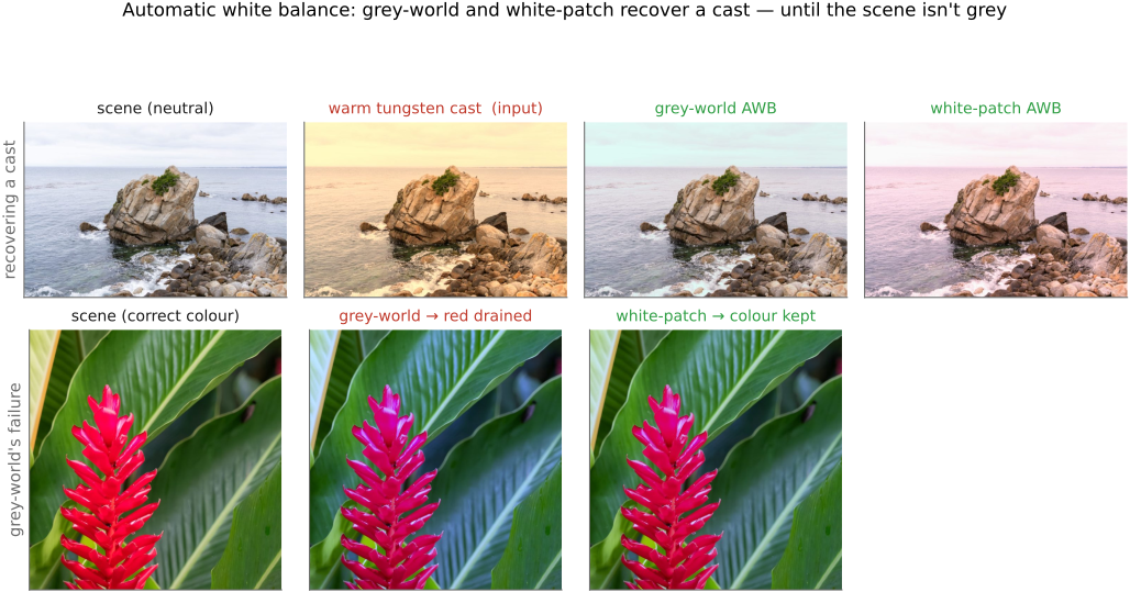
fig-white-balance-real · white balance computed from scratch (von Kries per-channel gain in linear light): a warm-casted photo corrected by gray-world vs white-patch/max-RGB, with the recovered channel gains (PS1) ✅
▸8.11 File formats and compression⧉
fig-jpeg-pipeline
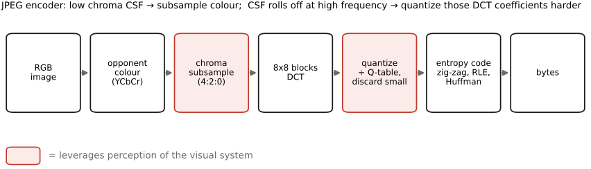
fig-jpeg-pipeline · the JPEG encoder — RGB → opponent color → chroma subsample → 8×8 DCT → quantize → entropy code (File formats, BASIC) 🟨
fig-dct-basis
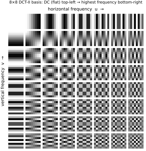
fig-dct-basis · the 8×8 DCT-II cosine basis (DC top-left → high frequency bottom-right) 🟨
fig-chroma-subsampling
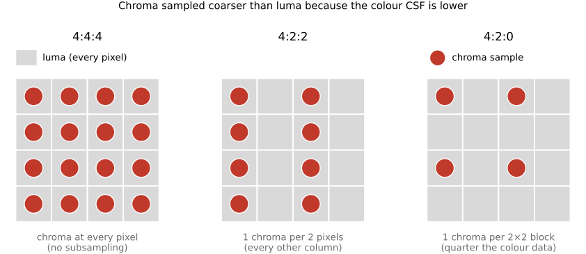
fig-chroma-subsampling · chroma subsampling grids 4:4:4 / 4:2:2 / 4:2:0 (chroma sampled coarser than luma) 🟨
fig-jpeg-artifacts
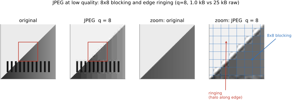
fig-jpeg-artifacts · JPEG blocking & ringing at low quality (original vs q=8, zoomed crop) 🟨
fig-jpeg-quality-levels
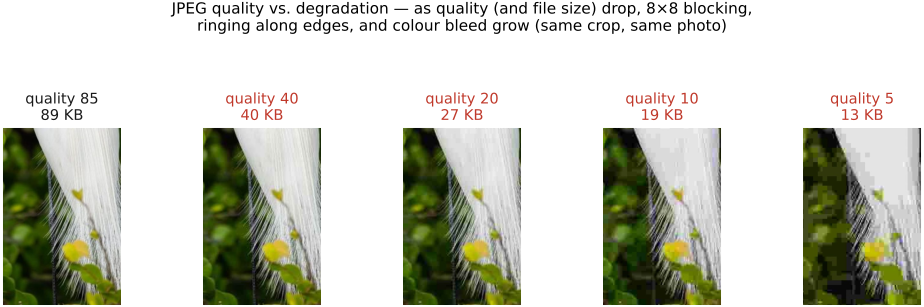
fig-jpeg-quality-levels · JPEG quality sweep (q=85→40→20→10→5): the same photo's edge-crop at each quality with the whole-image file size beneath — degradation grows as size drops (File formats, BASIC) 🟩
8.11.5 Making JPEG differentiable⧉
▸8.12 Recap ISP, non-destructive editing:⧉
fig-isp-block-diagram
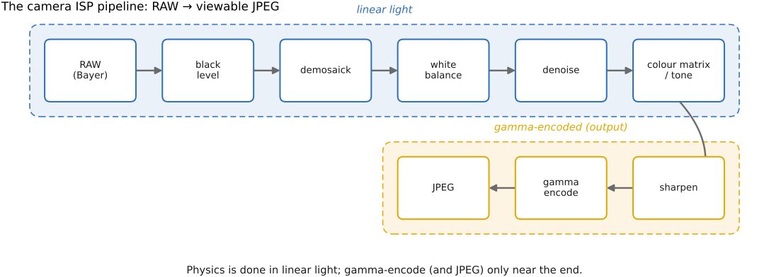
fig-isp-block-diagram · the ISP pipeline: RAW → black level → demosaick → white balance → denoise → tone/color → sharpen → gamma → JPEG (Recap ISP, BASIC) 🟨
8.12.2 Two stages this part did not teach⧉
8.12.3 Real ISPs⧉
8.12.4 Pipeline design and tuning⧉
8.12.5 The ISP, evolving: traditional → learned → generative⧉
▸8.13 A raw developer in the browser⧉
• the part's claim made drivable: a raw editor is a programmable ISP exposed to the user
• two suggested experiments: Profile → Neutral (the beauty curve's contribution), and the clipping overlay on a bright sky (recoverable vs gone → bracketing, MULTIPLE EXPOSURE IMAGING)