BookNotesSlidesP-sets Syllabusdraft · v0.2.49.1
💬Comments welcome. To leave a note, select any text and click the note / highlight button that pops up — or open the panel with the tab at the top-right (‹). Notes are visible only inside our private review group.
Computational Photography, an AI-powered Slopendium — 06 Linear methods and Fourier analysis
expand to📖 Full book outline1 parts · 9 chapters · 89 sections · 39 figures embedded · 2 placeholders · double-click a figure to enlarge
▸Part 6 LINEAR METHODS AND FOURIER ANALYSIS⧉
<!--uid: linear-methods-and-fourier-analysis-->
Linear methods deserve a part of their own for three reasons. (1) Many processes in photography are genuinely linear: incoherent imaging is linear in intensity, coherent imaging is linear in amplitude. (2) Even when a process is not linear it can usually be linearized for small quantities (thin-lens/paraxial optics, motion magnification). (3) Linear algebra offers a plethora of powerful tools for processing images and solving inverse recovery problems, both practical and conceptual. This part develops the linear-systems vocabulary (convolution, Fourier, sampling, pyramids) and the linear-algebra view of image formation and its inversion (imaging as a linear system, linear inverse problems, fundamental limits).
▸6.1 Introduction to forward and inverse linear methods⧉
6.1.2 Running the blur backward: the idealized case⧉
6.1.3 The catch: noise and ill-conditioning⧉
6.1.6 A different challenge: sampling and aliasing⧉
6.1.7 What the measurement determines⧉
▸6.2 Convolution⧉
⬜ figure not yet created
kernel sliding over an image fig-convolution-slide
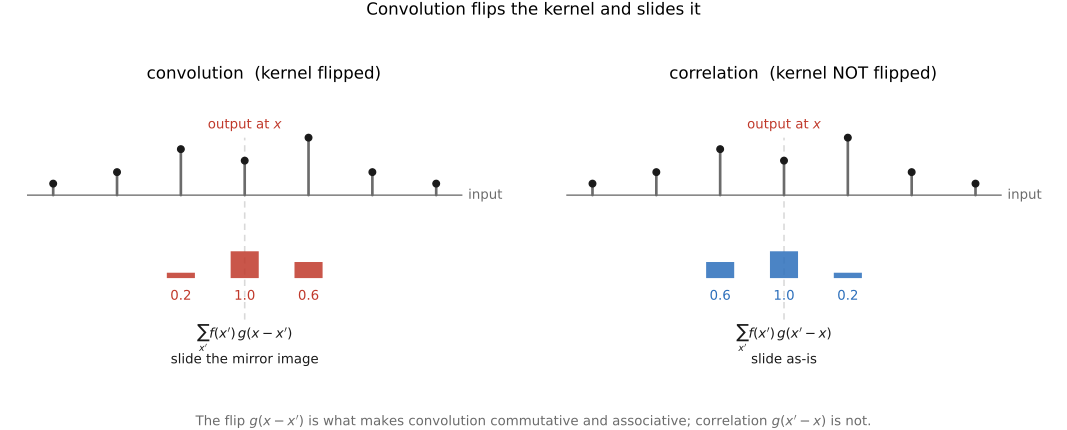
fig-convolution-flip
fig-convolution-flip · the flip: where-from vs where-to — convolution `g(x−x')` vs correlation 🟨
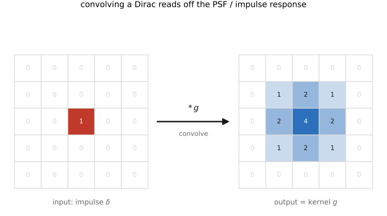
fig-psf-impulse
fig-psf-impulse · impulse in → kernel out: convolving a Dirac reads off the PSF / impulse response 🟨
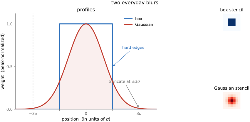
fig-blur-zoo
fig-blur-zoo · box vs Gaussian kernels — profiles + 2-D stencils, Gaussian truncated at ~3σ 🟨
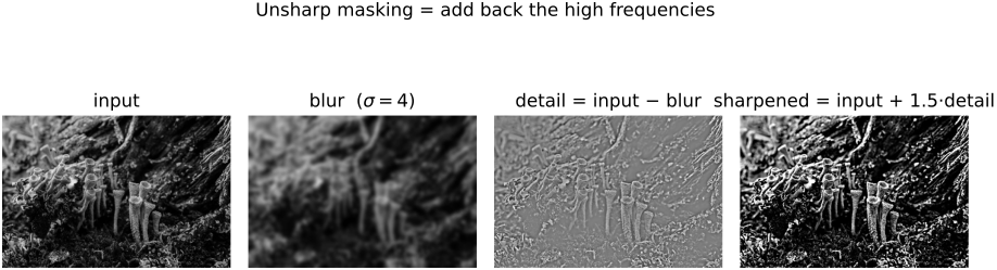
fig-unsharp-mask
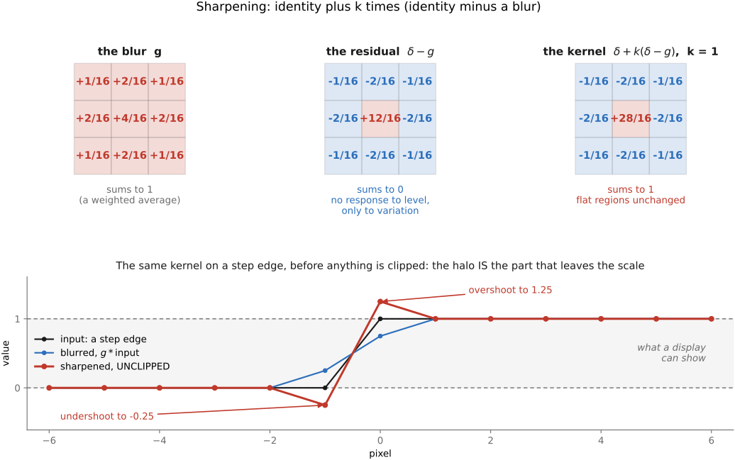
fig-unsharp-mask · unsharp-mask decomposition: input − blur = detail (high-pass), output = input + k·detail 🟨
fig-sharpen-kernel
fig-sharpen-kernel · the sharpening kernel δ − blur as a +center / −surround stencil 🟨
fig-separable
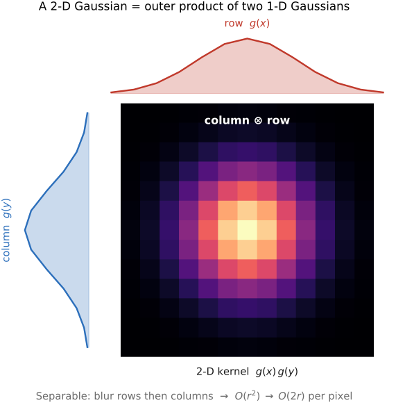
fig-separable · separability — a 2-D Gaussian = 1-D ⊗ 1-D (blur rows then columns); O(r²) → O(2r) 🟨
fig-gradient-sobel
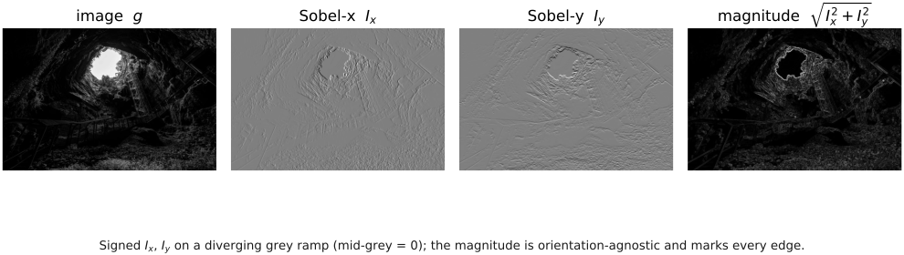
fig-gradient-sobel · Sobel x / y → gradient magnitude (edge strength) on an image 🟨
fig-convolution-probability
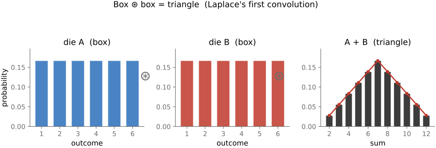
fig-convolution-probability · convolution as the sum of random variables: box ⊛ box = triangle (two dice) 🟨
equations
convolution (I*g)(x) = Σ I(x')·g(x−x')
Gaussian g(x) ∝ exp(−x²/2σ²)
unsharp out = in + k·(in − blur(in))
sharpening kernel δ − g
6.2.4 Convolution as a sum of translated images⧉
6.2.9 Linear sharpening⧉
6.2.11 Is imaging blur usually a shift-invariant convolution?⧉
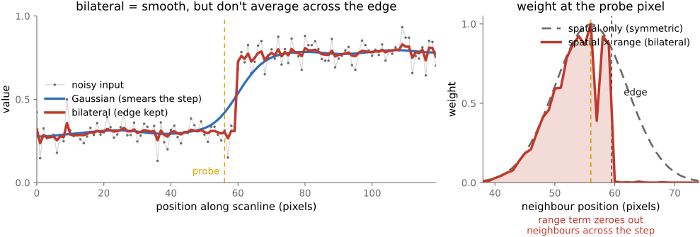
6.2.12 Fixed and data-dependent weights⧉
▸6.3 Fourier⧉
fig-fourier-basis-matrix
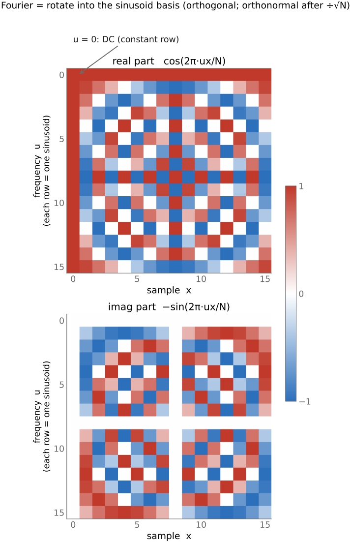
fig-fourier-basis-matrix · the DFT as a change-of-basis matrix (real & imaginary parts) 🟨
fig-sine-eigenvectors
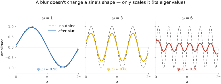
fig-sine-eigenvectors · sine waves are the eigenvectors of convolution: same wave out, only amplitude/phase change 🟨
fig-motion-blur-calculator
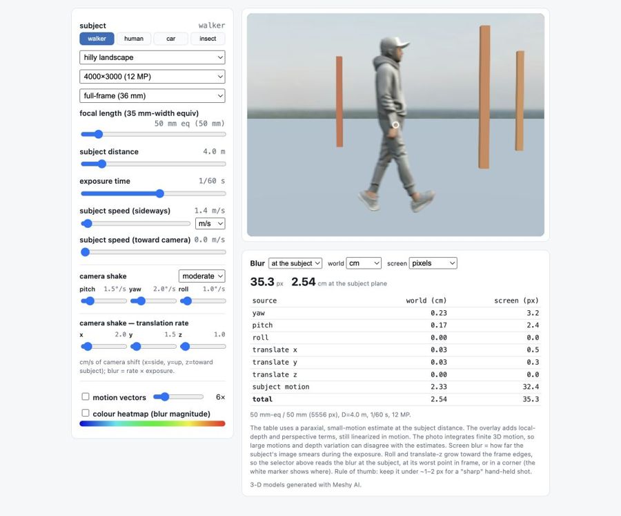
fig-motion-blur-calculator · live motion-blur calculator: a 3-D scene (walking figure or a car) imaged by a virtual camera, the blur rendered by **temporal supersampling** (many instants across the exposure, averaged). Set resolution / sensor / focal length (35 mm-equiv) / distance / exposure, add camera-shake **rates** in rotation (pitch/yaw/roll) and translation (x/y/z) plus a subject speed; the readout gives the blur at the subject in world (cm/m/in) and screen (px / % width) units, broken down by source. A per-pixel **G-buffer** (depth + subject mask) drives exact motion-vector arrows and a blur-magnitude heatmap: the subject carries its own motion, the background only camera shake. Environment backdrops + car color picker. Static fallback is a screenshot. *3D models generated with Meshy AI.* ✅
fig-fourier-magnitude-phase
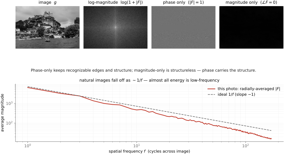
fig-fourier-magnitude-phase · an image's Fourier magnitude & phase, and the phase-swap demo (phase carries structure) 🟨
fig-compact-space-frequency
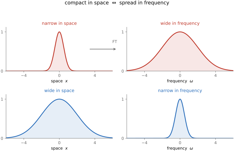
fig-compact-space-frequency · compact in space ⇔ spread in frequency (narrow vs wide Gaussian and its transform) 🟨
fig-aliasing
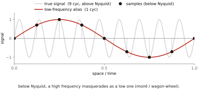
fig-aliasing · sampling a sine too coarsely → aliasing (high frequency folds to a low one) 🟨
fig-sampling-comb
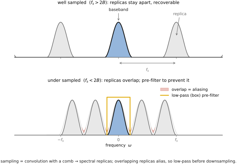
fig-sampling-comb · sampling = multiply by a comb → spectral replicas; pre-filter (low-pass) before downsampling 🟨
fig-sinc-vs-practical
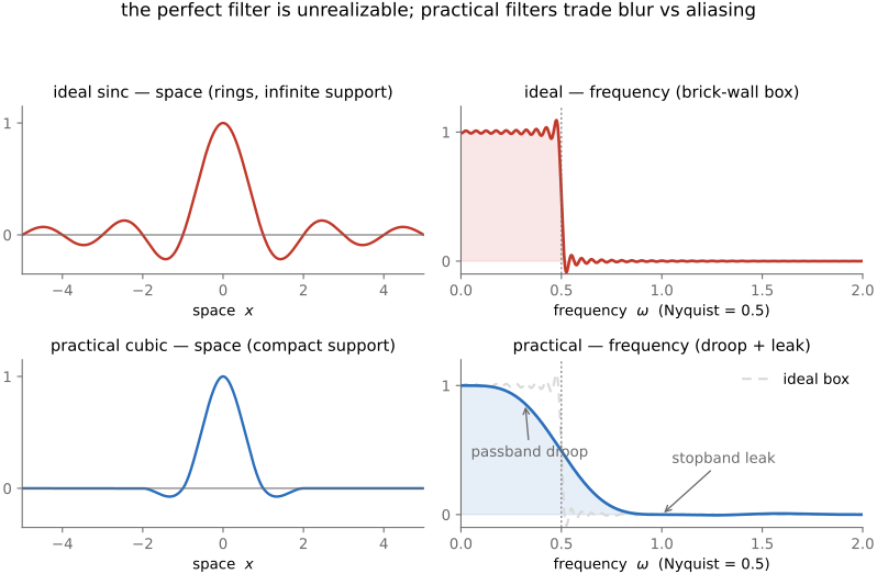
fig-sinc-vs-practical · ideal sinc reconstruction vs a practical filter, in space and frequency 🟨
fig-deblur-preview
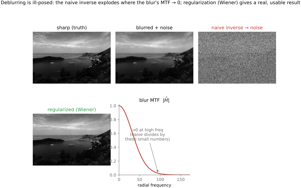
fig-deblur-preview · the deblur preview: sharp → blurred + noise → naive inverse amplifies noise; MTF 🟨
fig-diagonalize-2x2
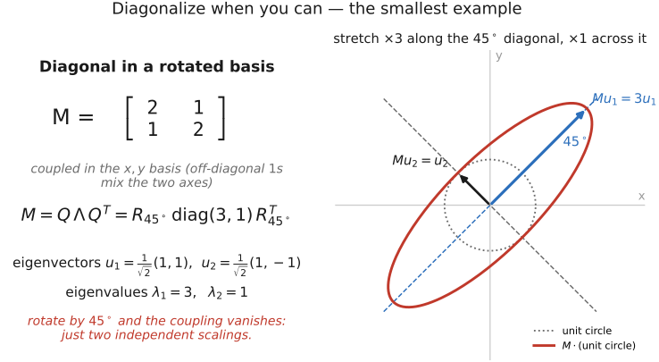
fig-diagonalize-2x2 ·
fig-fourier-conventions
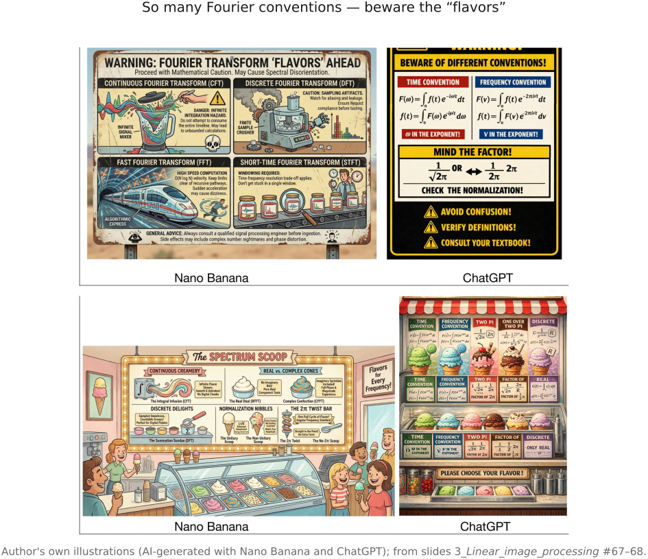
fig-fourier-conventions ·
fig-heat-diffusion-1d
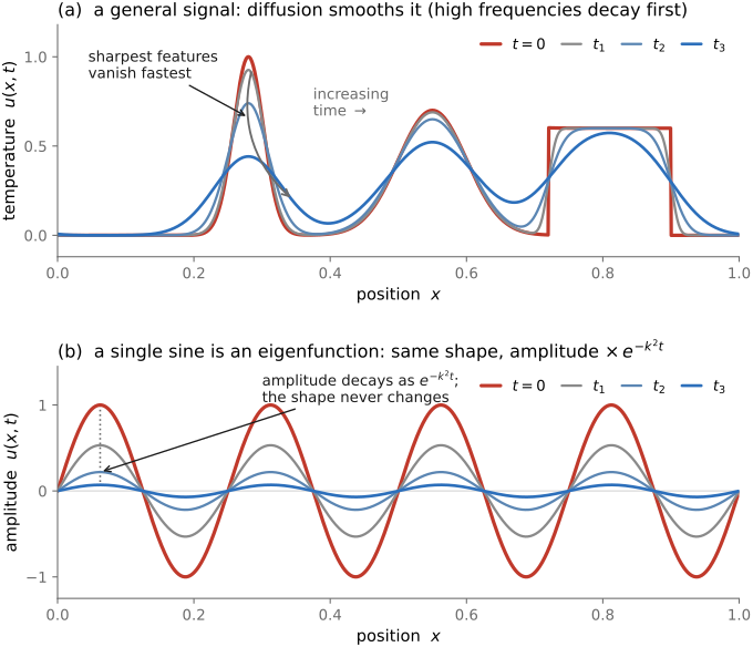
fig-heat-diffusion-1d ·
equations
DFT Î(u) = Σ I(x)·e^{−2πi ux/N}
Euler e^{iθ} = cos θ + i sin θ
convolution theorem ℱ{I*g} = ηĝ
eigen-relation g * e^{iωx} = ĝ(ω)·e^{iωx}
Nyquist — sample > 2× the highest frequency
6.3.5 The tiniest Fourier transform in the West⧉
6.3.8 A small bestiary of transforms⧉
6.3.9 Optics and Fourier⧉
6.3.10 MTF: a lens's frequency response⧉
6.3.15 Convolution by FFT⧉
▸6.4 Sampling, downsampling, and aliasing⧉
• promoted from a section of [[#Fourier]] into its own chapter (it earns one): a digital image is a **sampling** of a continuous scene, and detail finer than the grid **aliases** — folds down to a wrong, low frequency (moiré, wagon-wheel).
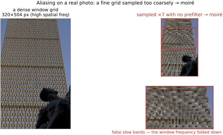
• **aliasing = a high frequency in disguise** (sine sampled below 2×/cycle → looks like a slower sine); 2-D version = moiré on a facade. Figures: `fig-aliasing`, `fig-aliasing-photo`.
• **Nyquist–Shannon**: sample at >2× the highest frequency; the **Nyquist frequency** is half the sampling rate; above it folds down irreversibly.
• **frequency-domain mechanism**: sampling is **multiplication by a Dirac comb** in space, so by the convolution theorem it becomes a **convolution in Fourier** — but by an unusually *simple* spectrum. The comb is **self-dual**: the Fourier transform of a Dirac comb is **another train of Diracs** (spaced at the sampling rate). And that is exactly why sampling is *easy* to reason about in Fourier: convolving by a single Dirac is just a **shift**, so convolving by a *train* of Diracs is just a **sum of shifted copies**. The spectrum is simply **replicated** at every multiple of the sampling rate — no smearing, just shifts. (This is the payoff of Fourier being built on the **shift theorem**: the one convolution that would otherwise be messy collapses into pure translation.) Band-limited copies sit apart; too-wide copies **overlap** = aliasing (`fig-sampling-comb`). Big lesson **L4.13**.
• **cure**: low-pass **pre-filter** (blur) *before* downsampling. Interactive demos: `fig-sampling-1d-demo` (1-D sampling/aliasing/pre-filter, tick-marked samples + spectrum) and `fig-sampling-2d-demo` (downsample the Prudential facade with/without pre-filter → moiré on/off).
• sidebars: aliasing **without** Fourier (pixel = area average); aliasing **on purpose** (KinéCam moiré encodes camera motion).
• **ideal sinc** reconstruction (perfect frequency box ⇒ infinite spatial ripple) is unreachable; practical filters compromise (`fig-sinc-vs-practical`) — handed off to [[#Resampling and upsampling]].
• xref: built on [[#Fourier]]; reconstruction / upsampling lives in [[#Resampling and upsampling]].
6.4.1 Aliasing: a high frequency in disguise⧉
6.4.2 Nyquist and the sampling theorem⧉
6.4.3 In two dimensions, aliasing has a direction⧉
6.4.4 Sampling in the frequency domain: spectral replicas⧉
6.4.5 Seeing it: sampling and pre-filtering, hands on⧉
6.4.6 The ideal reconstruction filter: sinc, and why it is unreachable⧉
▸6.5 Resampling and upsampling⧉
fig-resample-forward-inverse
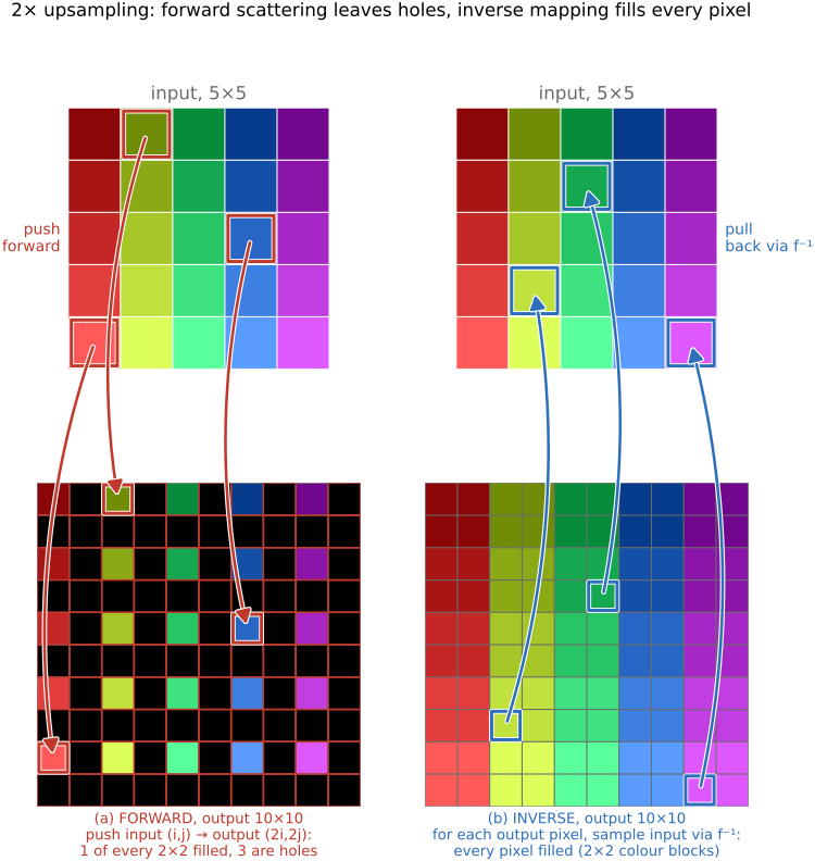
fig-resample-forward-inverse · concrete 2× upsampling on a 5×5 → 10×10 rainbow grid: FORWARD pushes input (i,j)→output (2i,2j) so 1 of every 2×2 output block is filled and 3 are black holes (regular lattice of gaps); INVERSE loops output, samples input via f⁻¹ (nearest) → every pixel filled (2×2 color blocks). Forward leaves holes, inverse fills everything (Resampling, BASIC) ✅
fig-linear-interp-1d
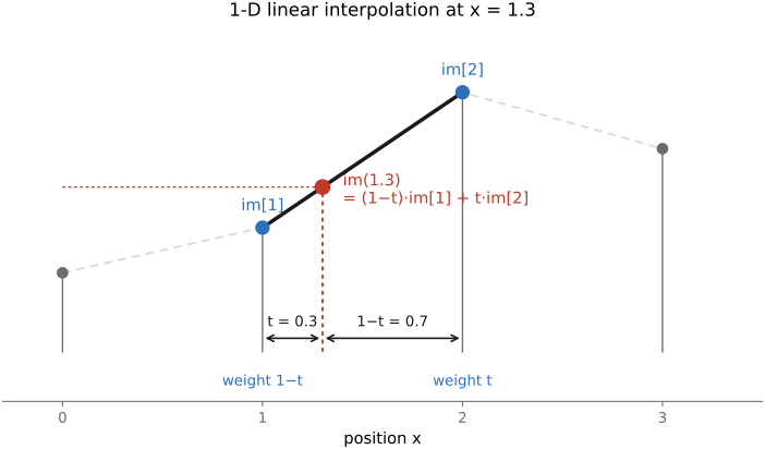
fig-linear-interp-1d · 1-D linear interpolation — `im[1.3]` from its two neighbors 🟨
fig-bilinear
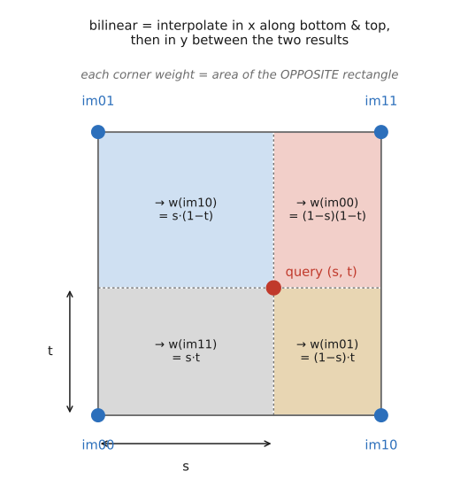
fig-bilinear · bilinear interpolation — the 4-neighbor weighting on the unit square 🟨
fig-resample-kernels-real
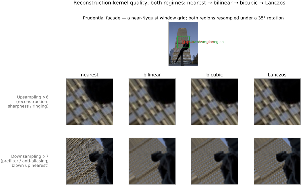
fig-resample-kernels-real · the kernel ladder on a REAL photo (Boston skyline + rainbow) resampled under a 35° rotation, magnified on a detail: nearest (blocky) → bilinear (smeared) → bicubic (edges restored) → Lanczos (sharpest) — adds Lanczos + the rotation case to `fig-interp-comparison` ✅
fig-reconstruction-pipeline
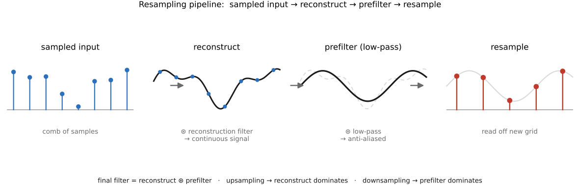
fig-reconstruction-pipeline · the resampling pipeline: sample → reconstruct → prefilter → resample 🟨
fig-aliasing-photo
fig-aliasing-photo · aliasing/moiré on a real photo: a window-grid facade decimated with no prefilter folds into moiré bands — the 2-D, real-image companion to `fig-aliasing` (Sampling and aliasing) ✅
equations
1-D linear interp
general resample out(x) = Σ I(x')·k(f⁻¹(x) − x')
Lanczos `sinc(πx)·sinc(πx/a)`
Mitchell–Netravali cubic (B, C)
6.5.5 Nearest neighbor⧉
6.5.13 Resampling and encoding⧉
6.5.15 Practical implementation choices⧉
▸6.6 Pyramids and wavelets⧉
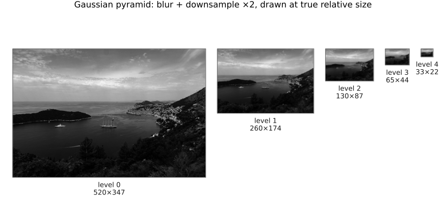
fig-gaussian-pyramid
fig-gaussian-pyramid · the Gaussian pyramid — repeated blur + downsample tower (Pyramids, BASIC) 🟨
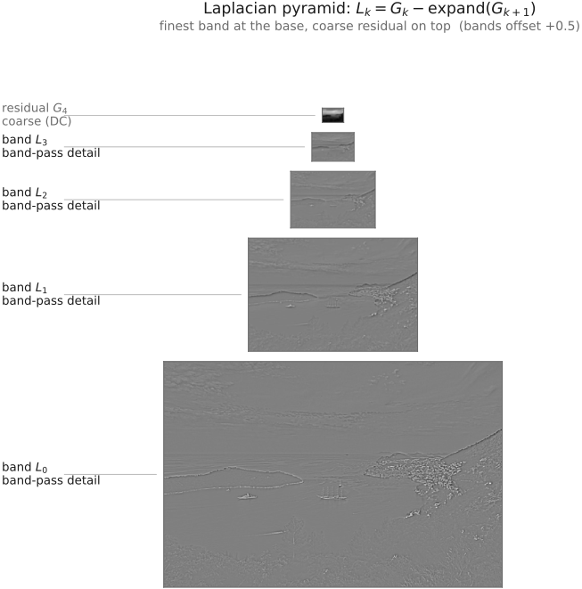
fig-laplacian-pyramid
fig-laplacian-pyramid · the Laplacian pyramid — band-pass levels (G_k − expand(G_{k+1})) 🟨
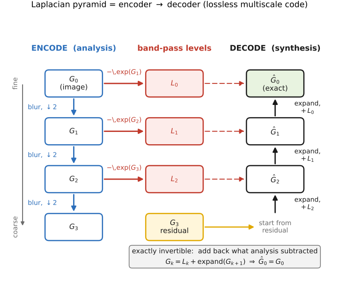
fig-pyramid-encode-decode
fig-pyramid-encode-decode · the Laplacian pyramid as an encoder → decoder (exact reconstruction) 🟨
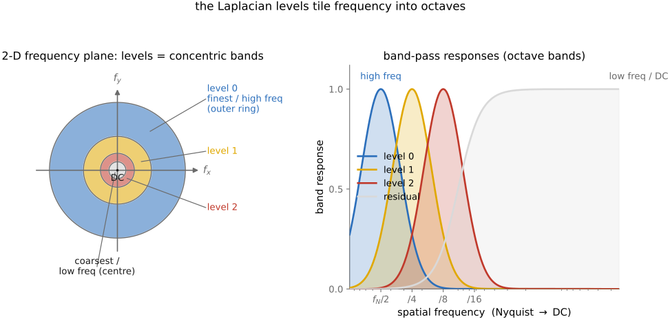
fig-pyramid-frequency-bands
fig-pyramid-frequency-bands · each pyramid level = a frequency band (concentric Fourier rings) 🟨
fig-kernel-spectra
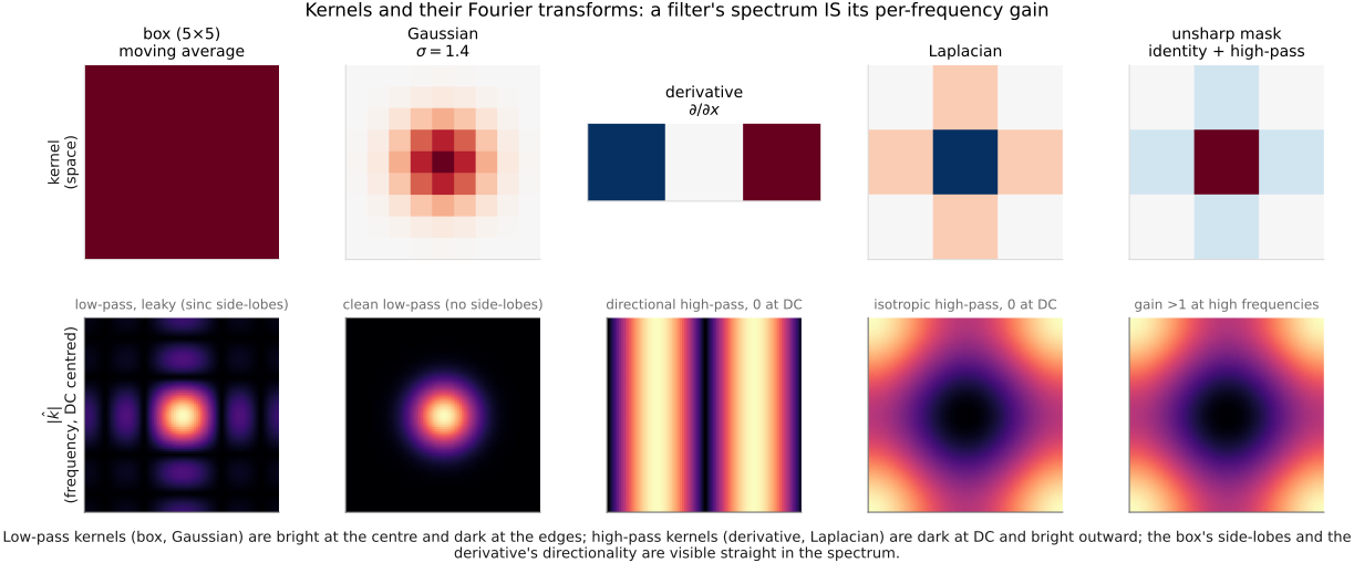
fig-kernel-spectra · five common kernels (box, Gaussian, derivative ∂/∂x, Laplacian, unsharp mask) shown in space and as their Fourier magnitudes — a filter's spectrum IS its per-frequency gain (low-pass leaky vs clean, directional/isotropic high-pass, boosting) ✅
fig-coring
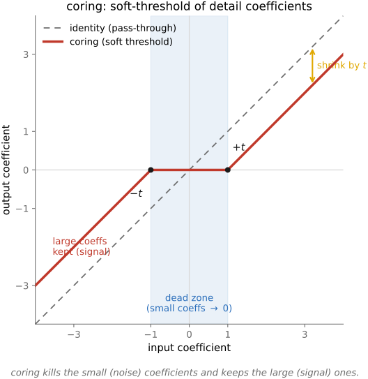
fig-coring · coring — zero the small detail coefficients (noise), keep the large ones 🟨
equations
reduce / expand (blur + ↓2 / ↑2 + blur)
L_k = G_k − expand(G_{k+1})
reconstruction G_k = L_k + expand(G_{k+1})
6.6.10 Pyramid blending⧉
6.6.11 Other applications⧉
6.6.12 Coarse-to-fine methods⧉
▸6.7 Image formation as a linear system⧉
6.7.3 How solvable is an imaging problem?⧉
6.7.4 Regularization⧉
6.7.7 Other forms of linearity, and multilinearity⧉
6.7.8 Designing measurements for recovery⧉
▸6.8 When linearity breaks down⧉
⬜ figure not yet created
deconvolution in linear vs gamma-encoded values [fig-deconv-gamma-linear]. fig-deconv-gamma-linear
▸6.9 Efficient linear solvers⧉
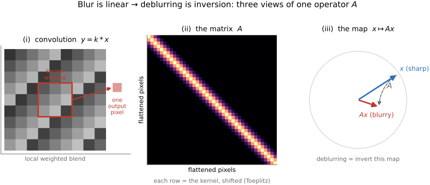
fig-deblur-linear-inversion
fig-deblur-linear-inversion ·
fig-deblur-preview
fig-deblur-preview · the deblur preview: sharp → blurred + noise → naive inverse amplifies noise; MTF 🟨
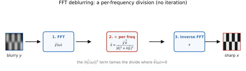
fig-deblur-fft-solver
fig-deblur-fft-solver ·
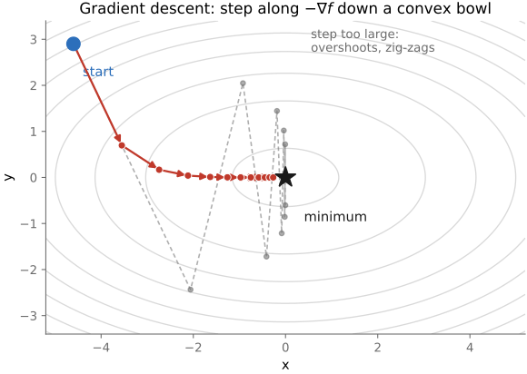
fig-gradient-descent
fig-gradient-descent · descent path on a convex-bowl contour (−∇f steps); too-large step overshoots (Optimization) 🟩
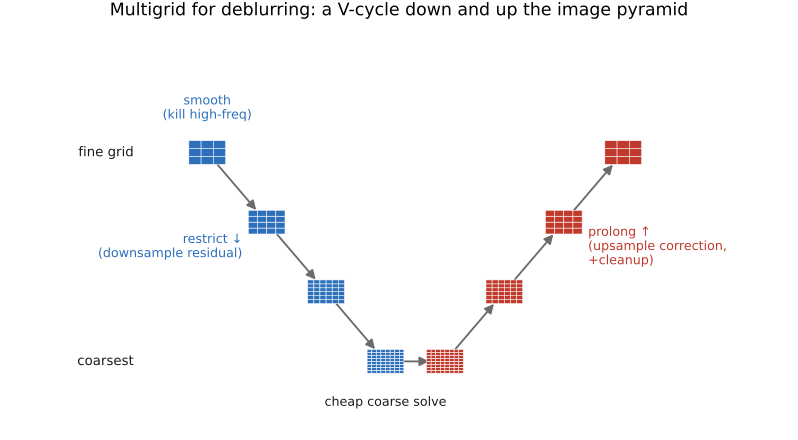
fig-deblur-multigrid-vcycle
fig-deblur-multigrid-vcycle ·
equations
normal equations $(A^\top A+\lambda L)x=A^\top y$
gradient $\nabla f=A^\top(Ax-y)$
gradient step $x_{t+1}=x_t-\eta A^\top(Ax_t-y)$
matrix-free product $A^\top A v=\tilde k*(k*v)$
flipped-kernel transpose $A^\top y=\tilde k*y$
regularized per-frequency FFT solve $\hat x=\overline{\hat k}\hat y/(|\hat k|^2+\lambda|\hat L|^2)$.
6.9.1 The problem, and the one trick⧉
6.9.2 Direct methods, and why they wall out⧉
6.9.3 Basic iterative solvers⧉
6.9.4 Conjugate gradient⧉
6.9.5 Preconditioning⧉
6.9.6 Multigrid⧉
6.9.7 Which solver when, and the edges⧉