Lecture Notes 9 — Morphing⧉
Course notes cut from Computational Photography, an AI-powered Slopendium for this lecture. Each section links back to its home in the book; sections marked optional go beyond what the lecture needs.
Contents · 24 sections on this page, from 8 chapters of the book
Titles jump to the section below; ↗ opens it in the book.
Color TLDR⧉
optionalGamma, cross-fading, and linear operations⧉
The single most common way the encoding boundary bites is the most innocent-looking: interpolating between two colors. A cross-fade, a gradient, an alpha blend, an antialiased edge, all average two colors, and averaging is a linear-light operation. Do it on gamma-encoded values and you do not just get a slightly-off brightness, you get false intermediate colors: fade encoded red to encoded green and the midpoint goes through a muddy dark brown instead of a bright yellow, because the encoding pulls the sum down before the two channels can both be high at once. The fix is the usual one, decode, interpolate, re-encode, and the difference is not subtle once you look (John Novak's "What every coder should know about gamma" is the definitive visual demonstration).
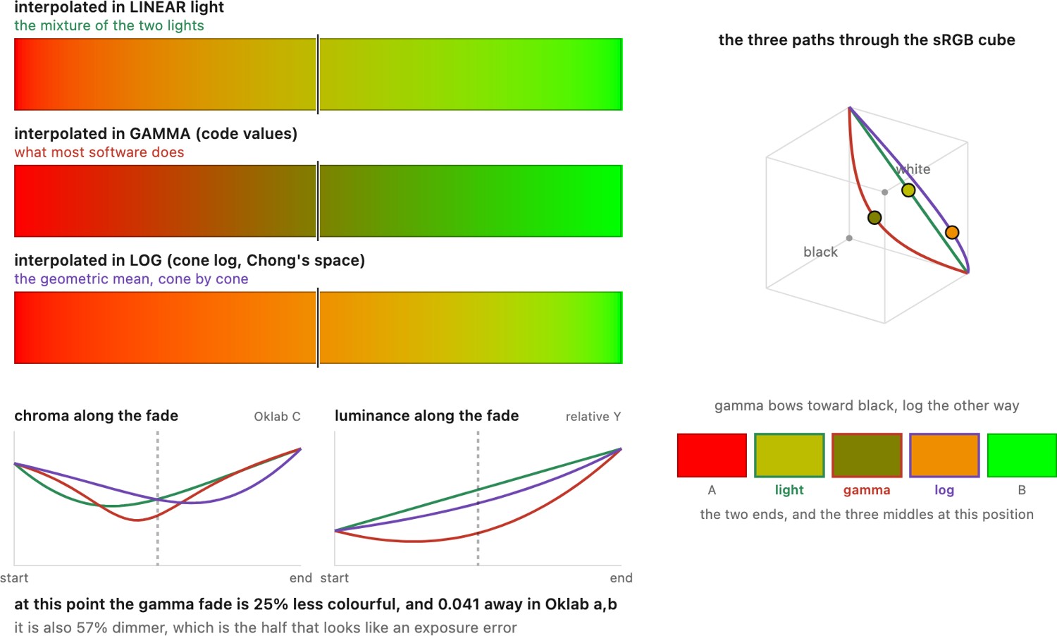
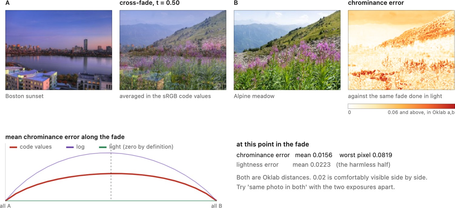
Flat patches make the argument; photographs make it land, because a photograph has thousands of chromaticities and the error goes where the color is. The next figure runs the same three averages on two pictures, and maps what the choice costs in chrominance alone (the figure).
Warping, morphing, and lagrangian approaches⧉
optionalStraightening a façade, aligning a burst and moving a face landmark all change where image samples contribute. A warp specifies that geometry; resampling determines the output values. Keeping those two tasks separate lets us reuse one sampling implementation for many kinds of edit.
Chapter 11.1, Warping defines forward and backward maps, boundaries and interpolation. Chapter 11.2, Antialiasing for complex transforms handles footprints that stretch or rotate across the image. A destination pixel may cover many source samples, so a sharper interpolator alone cannot prevent aliasing.
Chapter 11.3, Morphing combines correspondence with appearance blending. Chapter 11.4, Morphable models restricts possible shapes using a learned population model, while Chapter 11.5, Shape-preserving warping penalizes local deformation. These constraints can improve an edit without guaranteeing physical validity or preventing every fold.
Chapter 11.6, Perspective distortion and its correction separates planar rectification, virtual camera rotation and local perceptual adjustments. None can recover unseen surfaces from a single photograph without additional information or inference.
The distinction between changing values and moving content is related to two descriptions of fluid motion. An Eulerian description observes a fixed location, like a weather station measuring the air that passes it. A Lagrangian description follows material, like a balloon drifting with that air. A tone curve changes values on a fixed image grid. A geometric warp instead describes where scene content moves. The implementation may still visit a fixed output grid through backward mapping; the Lagrangian analogy concerns the motion being represented. Video compression shows why the distinction matters in practice. Coding each frame as its per-pixel difference from the previous one is an Eulerian scheme, and it wastes bits whenever something moves, since a moving edge produces large differences at every pixel it crosses. Motion-compensated coding, as in the MPEG and H.264 families, predicts each block from where its content was in the previous frame and codes only the correction, which is cheap when the motion is well described (Chapter 30.2, Video compression and motion compensation).
That separation also explains the organization of these chapters. One question is how to specify the map: a few parameters, sparse landmarks, a deformation mesh or a dense field. Another is how to apply it to sampled data. Translation, lens correction, stabilization and a facial morph can share a resampling engine even though their maps come from different models. Matching pixels across space and time addresses estimating those correspondences; this part develops their use to transport image content.
Warping⧉
PS5 implements resampling kernels and Beier–Neely segment warps. → Chapter 1.5, Problem sets (appendix).
Print a photograph onto a sheet of rubber and stretch it: pinch a corner, bow the middle, slide one edge. The pixels glide to new positions and the picture rides along: a face slims, a bent line straightens, a tilted building stands up. Nothing about the colors changed; what changed is where each color lives. That is a warp, and it is the single operation underneath a large range of this book's geometry: lens-distortion correction, video stabilization, panorama reprojection, morphing, image-based rendering, even the cosmetic "liquify" slider. One primitive, reused everywhere, which is exactly why it opens this part.
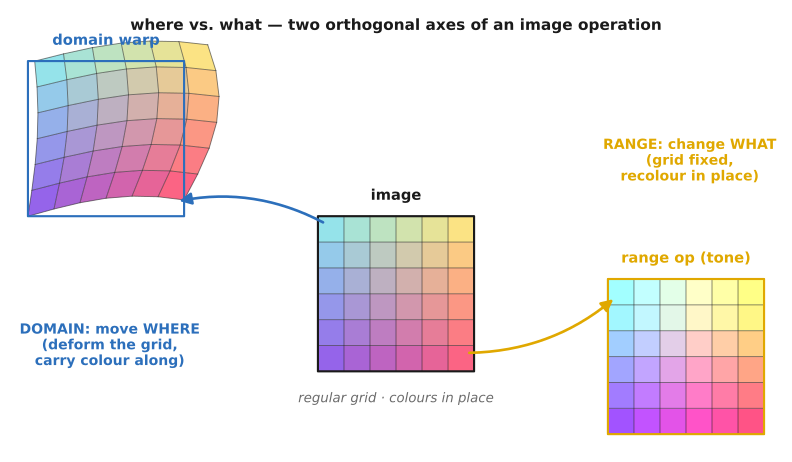
Formally a warp is a map of the image domain: a function $f:\mathbb{R}^2\to\mathbb{R}^2$ that moves positions while leaving the range (the colors) untouched. If the input had color $c$ at $(x,y)$, the output has that same $c$ at $f(x,y)$. It is the geometric twin of a point operation: a point operation edits the range (the colors) and leaves the domain fixed; a warp edits the domain (the positions) and leaves the range fixed.
The map and the sampler have separate responsibilities. The map supplies coordinates; the sampler reconstructs values and filters the source footprint. A valid coordinate alone does not establish visibility or adequate antialiasing.
Warping is a domain transform: move where, not what⧉
Hold onto the rubber-sheet image, because it is the correct mental model for every warp in the book, from a sub-pixel lens-distortion correction to a full perspective rectification to "slim the subject." The warp deforms where pixels live and leaves their colors alone. Contrast it once more with a tone or point operation, which recolors each pixel in place: warping is the domain operation to that range operation, and the two are orthogonal; you can do either without the other, and morphing (later in the part) does both at once, a domain warp plus a range cross-fade.
Before building the machinery, note why this one primitive is everywhere, because the motivation is the whole reason the chapter comes first. Optical-aberration and lens-distortion correction are warps. Video stabilization is a warp (a different one per frame). Panorama reprojection, aligning each photo to a reference view, fixing the apparent shift of a rotated camera, is a warp. Wide-angle distortion correction, morphable face models, image-based rendering, the cosmetic slim: all warps. Learn to transport pixels along a map once and you have the engine for all of them. That observation, that nearly every geometric operation in the book is "build a map, then move the pixels along it," is the part's central lesson L17.
Almost every geometric algorithm in the book has the same two-part shape: first establish a coordinate map between two images (or between an image and a target frame), then transport the pixels along it. This part builds that machinery and its first uses: warping makes the map explicit and applies it, perspective rectification solves the map (a homography) from geometric constraints, and morphing interpolates between two maps. The same shape recurs across the book: panorama stitching estimates the map from matched features (in the multiple-exposure part), optical flow estimates a dense map from brightness constancy (in the matching part), and stabilization smooths a map over time while frame interpolation renders along one (in the video part). Separating the two halves, what the map is versus how you transport pixels through it, is what lets one transport engine (inverse warp + resample, built in the next two sections) serve this part and recur throughout the book; only the map changes from task to task. (L17 is registered in the part introduction, Warping and morphing; this chapter is the transport engine, and the chapters that follow are different ways of finding the map.)
Forward vs inverse warping: why output-driven wins⧉
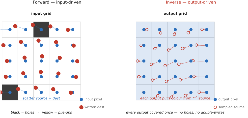
We met forward and inverse mapping for scaling in Chapter 6.5, Resampling and upsampling, and the conclusion carries over to any warp $f$. Pushing each input pixel to $f(x,y)$ leaves holes where the warp stretches and piles pixels up where it compresses. Looping over the output pixels instead, and pulling each one back through the inverse map,
fills every output pixel exactly once, and leaves a single question: how to read the input at the fractional location $f^{-1}(x,y)$ (Figure 11.1.2).
for each output pixel (x, y):
    (x', y') = f⁻¹(x, y)               # pull back to the source location
    out[x, y] = resample(in, x', y')   # read in at the fractional spot
Forward splatting remains useful when only a forward map is known, as with optical flow, but it then needs explicit handling of holes and overlaps.
An invertible affine or projective map has a matrix inverse. A fitted map may be singular or poorly conditioned, however, and a free-form field can fold or leave gaps. Forward flow cannot generally be inverted by negating it at the same coordinates: corresponding vectors live at different locations. Estimate a backward field or invert/splat with explicit visibility and coverage handling. Occluded or newly exposed content has no valid correspondence.
One more practical point that is not a corner case: $f^{-1}(x,y)$ can land outside the input. You must pick a boundary policy: zero/black padding, clamp-to-edge (replicate the border pixel), mirror, or mark as undefined (transparent, via an alpha channel). This matters constantly, because rectification and stabilization both produce outputs whose corners read past the original image border. Reading off the edge is the common case, not the exception.
Specifying the warp I: parametric models and the degrees-of-freedom (DOF) ladder⧉
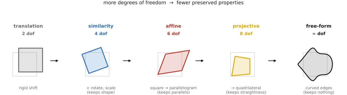
optionalWe have a transport engine; we now need maps $f$ to feed it. The easiest maps are parametric, low-parameter functions you fit to a handful of correspondences and then apply everywhere. They form a natural degrees-of-freedom ladder, each rung adding freedom and, in exchange, giving up a preserved property (Figure 11.1.3).
At the bottom is translation (2 DOF), which preserves everything but absolute position. Add rotation and you get a rigid / Euclidean transform (3 DOF), which preserves lengths and angles. Add uniform scale and you get a similarity (4 DOF), which preserves angles and length ratios, that is, shape. Loosen further to an affine map (6 DOF),
which preserves parallelism and ratios along a line but no longer angles or lengths: straight lines stay straight, parallel lines stay parallel, and a square becomes a parallelogram. At the top of the practical ladder is the projective transform or homography (8 DOF),
which preserves straight lines only. Parallels may now converge to a vanishing point, and a square can become any quadrilateral. This is the rung that does genuine perspective, and it is the engine of the next chapter's rectification and of panorama stitching.
The homography looks non-linear in $(x,y)$ because of the division by $w'$, and that is exactly why we use homogeneous coordinates: in homogeneous coordinates it is a single $3\times3$ matrix multiply followed by the perspective divide, restoring linearity to the part that matters. A plane induces a homography between views even when the camera translates. Pure camera rotation also induces a homography, for points at any depth, provided the camera model is appropriate. These are two distinct reasons a homography can align images without a per-pixel depth map. We do not re-derive any of this here; the full development lives in FUNDAMENTALS: Pinhole, and the solve for $H$ from correspondences is built in Chapter 20.1, Manual panorama stitching from multiple views, whose homography machinery this chapter shares wholesale.
A nondegenerate affine fit needs three noncollinear point pairs; a homography needs four pairs in general position. Additional pairs support a least-squares fit, but outliers require rejection or a resistant objective. Normalize coordinates for a homography’s linear initialization, then evaluate geometric reprojection error. Chapter 12.5, Robustness: the ratio test and RANSAC develops the outlier handling.
The strengths and the limit are two sides of one coin. Parametric warps are global, smooth, and low-parameter, which makes them a good choice when the deformation really is rigid, affine, or projective: a flat surface, a rotating camera, a lens model. But by the same token they cannot express a local, free-form deformation such as a smile, a face morph, or a hand-drawn stretch of one limb. For that we need a field built from sparse, local control, which is the next section.
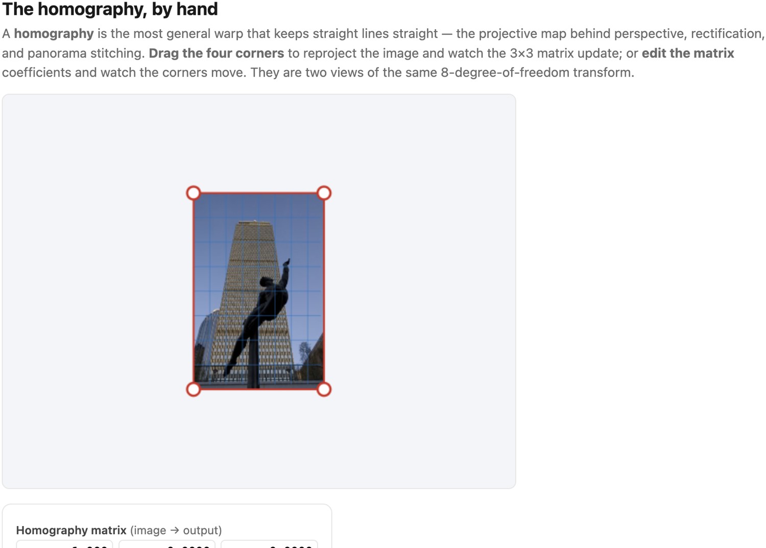
This is regression with the warp parameters as the unknowns. Each point pair contributes two coordinate equations. An affine fit is linear in its six parameters. A homogeneous linear initialization for a homography instead finds a null vector, commonly by singular value decomposition, before any geometric refinement. Counting equations explains the minimum number of pairs; checking their configuration explains why that count alone is insufficient.
Specifying the warp II: free-form warps from sparse correspondences⧉
When the deformation is local, the user supplies a sparse set of correspondences, such as a few control points or pairs of feature segments, and we must manufacture a dense warp field $f$, defined at every pixel, by interpolating those sparse constraints. Three constructions interpolate point controls, trading smoothness against locality: a triangulation, a grid of splines, and a thin-plate spline. Feature lines, which take segments instead of points, have their own section next, and a further idea layers a shape-preserving regularizer on top. The canonical reference across all of this is Wolberg's Digital Image Warping.
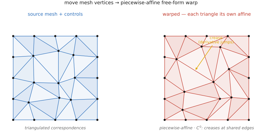
The simplest is the mesh / triangulation warp, which is piecewise-affine. Triangulate the control points (Delaunay, say); inside each triangle, the three vertex correspondences exactly determine an affine map (6 DOF, 3 points), so you warp each triangle by its own affine. It is fast, exact at the controls, and the standard morphing workhorse. Its weakness is that it is only $C^0$, continuous but creased, with derivative jumps at triangle edges, and its quality depends on how well the triangulation is chosen (Figure 11.1.5).
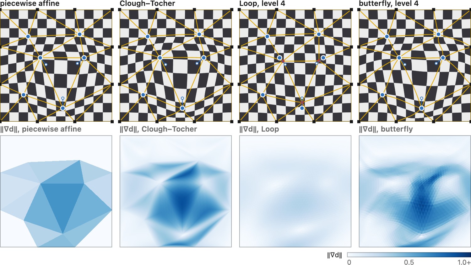
A triangulation can be made smooth without giving up its locality. The classical answer comes from finite elements: the Clough–Tocher interpolant splits each triangle into three at an interior point, fits a cubic on each of the three pieces, and matches them so that the field and its first derivatives are continuous across every edge Clough & Tocher 1965. It still passes through the control displacements, needs a gradient estimated at each vertex, and is the standard smooth interpolant for scattered two-dimensional data. Subdivision is another route. Subdivision surfaces smooth a triangle mesh by splitting every triangle into four, again and again, and replacing each value by a local average of its neighbors; Loop's rules converge to a surface that is twice differentiable except at vertices with an unusual number of neighbors Loop 1987 (Loop subdivision). Applied in the plane, to a displacement or any other value stored at the vertices, the same rules turn the creased piecewise-affine field into a smooth one. Davis, Levoy and Durand used exactly this to blend the views of an unstructured light field: each captured view gets a weight of one at its own vertex of a triangulation of the viewpoints and zero at the others, and subdividing those weights gives smooth blending functions where barycentric weights would crease Davis et al. 2012. The catch is that Loop's scheme approximates rather than interpolates: the limit does not pass through the vertex values, so a dragged control point does not end up where it was dropped. That is harmless for blending weights and wrong for a warp, which needs either a sparse linear solve for the vertex values whose limits hit the targets, or an interpolating scheme. The butterfly scheme keeps every existing vertex and places each new one with a stencil of eight neighbors shaped like a butterfly, so its limit passes through the controls Dyn, Levin & Gregory 1990 (butterfly); a modified version extends it to meshes of any connectivity and makes it continuously differentiable everywhere Zorin, Schröder & Sweldens 1996 (modified butterfly). Figure 11.1.7 compares the four on one set of controls (view compare). A map of the warp's derivative shows ridges along the triangle edges for Clough–Tocher and butterfly, which are only once differentiable, and none for Loop. Unsolved, Loop's limit misses a dragged control by up to about five percent of the image width and shrinks the whole warp; solving for the vertex values removes the miss (view loop). The last view shows the light-field use: one vertex at one and the others at zero, piecewise linear against Loop (view weights).
The first morph in a feature film used a different kind of mesh, a grid with splines between its nodes. For Willow (1988), in which a sorceress changes through a series of animals back into a woman, Doug Smythe at Industrial Light & Magic wrote a two-pass mesh warp Smythe 1990 (two-pass mesh warping). The artist lays a regular grid of control points over the first image and moves its nodes onto the matching features of the second. The two meshes have the same topology, so node $(i,j)$ of one corresponds to node $(i,j)$ of the other, and nothing needs to be triangulated. Between the nodes the warp is interpolated with cubic splines (Catmull–Rom splines in Wolberg's description), not with flat triangles, so the field is smooth across the grid lines and shows none of the creases of a triangulation Wolberg 1990 (Figure 11.1.8, stage grids). We follow the algorithm on a photograph in Figure 11.1.8, one step per stage.
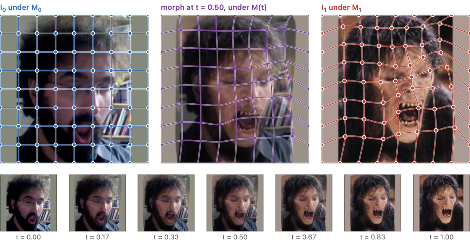
The warp itself is computed in two one-dimensional passes, following Catmull and Smith's separable scheme Catmull & Smith 1980. An intermediate mesh $M_I$ takes its $x$ coordinates from the destination mesh $M_1$ and its $y$ coordinates from the source mesh $M_0$. The first pass moves pixels only horizontally, from $M_0$ to $M_I$: a spline through each column of nodes gives, on every image row, the $x$ positions where the vertical grid lines cross that row in both meshes, and a spline through those crossings maps every $x$ of the row to its new position. The row is then resampled with a one-dimensional filter. The second pass does the same vertically, from $M_I$ to $M_1$ (Figure 11.1.8, stages pass1 and pass2).
mesh_warp(img, M0, M1):                       # M0, M1: grids of node positions, same size
    MI = nodes with x from M1 and y from M0
    for each row y of the image:                          # pass 1: horizontal
        xs0 = x where each column of M0 crosses row y     # spline through that column's nodes
        xsI = x where each column of MI crosses row y
        g = spline through the pairs (xs0, xsI)           # 1-D map for this row
        tmp[y, :] = resample_1d(img[y, :], g)
    for each column x of tmp:                             # pass 2: vertical
        ysI = y where each row of MI crosses column x
        ys1 = y where each row of M1 crosses column x
        h = spline through the pairs (ysI, ys1)
        out[:, x] = resample_1d(tmp[:, x], h)
    return out
Each pass is a set of one-dimensional resamplings, which are cheap and easy to filter well, and this mattered on the computers of 1988. The separable scheme has a known weakness: where the warp rotates a region by a large angle, the first pass squeezes it into a sliver before the second pass expands it again, the bottleneck problem of two-pass warps. For a rotation by $\theta$ the first pass compresses the region to $\cos\theta$ of its width and the second stretches it back by $1/\cos\theta$. The decomposition itself is exact; the loss comes from resampling a squeezed image, and it grows quickly with the angle: on a portrait, about 1 gray level of error against a one-pass warp at 30°, 4 at 60° and 12 at 80° (stage compare, which also sets the grid warp beside triangles and bilinear cells). The grid lines also must not cross, or the one-dimensional maps fold over. For a morph, the node positions are interpolated, $M(t)=(1-t)\,M_0+t\,M_1$, both images are warped to $M(t)$, and the two warped images are cross-dissolved (Chapter 11.3, Morphing; stage morph).
A grid trades freedom for smoothness and speed. The artist must work within the grid's topology and often moves many nodes to describe one feature, an edge that runs diagonally across the cells for instance. That burden is what Beier and Neely's feature lines, below, set out to remove Beier & Neely 1992. Later spline methods kept the grid but freed the controls: a tensor-product B-spline grid can be fitted to scattered points or lines, with a coarse-to-fine hierarchy of grids that adds detail only where the constraints require it Lee, Wolberg & Shin 1997.
For smoothness without creases, the thin-plate spline (TPS), a radial-basis-function interpolant. Fit a field that passes through the control displacements while bending as little as possible:
an affine "global" part plus a sum of radial basis functions centered at the control points $\mathbf{c}_i$. The thin-plate kernel $\phi(r) = r^2 \log r$ is the one that minimizes integrated second-derivative (bending) energy, giving the smoothest possible interpolant, with the literal physical analogy of a thin metal plate bent to pass through pins at the constraints. The weights $w_i$ (together with $A,\mathbf{t}$) come from a small linear system. The result is smooth everywhere, with no creases, but it has global support: every control point influences every pixel, so it can be less local than a mesh, and the solve costs roughly $O(n^2)$–$O(n^3)$ in the number of controls. It is the go-to for smooth medical and facial registration and for morphometrics, following Bookstein.
The catch shared by all these constructions is that interpolating positions alone lets shapes shear and squash unnaturally: drag one handle and an unconstrained fit will stretch and skew the whole region. The fix is a shape-preserving regularizer: as-rigid-as-possible (ARAP) Igarashi et al. 2005 or moving-least-squares (MLS) Schaefer et al. 2006 deformation, which keeps each local neighborhood close to a pure rotation so a dragged limb bends without stretching. That regularizer is important enough to get its own chapter: we defer it to Chapter 11.5, Shape-preserving warping and only flag here that plain position-interpolation is not shape-preserving.
Compose maps before resampling where possible. If forward maps are $f_1$ then $f_2$, the combined backward lookup is $f_1^{-1}\circ f_2^{-1}$. Repeatedly resampling the image adds blur and rounding. Test an identity map, an integer translation and an affine ramp; declare whether integer coordinates denote pixel centers.
For a thin-plate spline in two dimensions, a common basis is $\phi(r)=r^2\log r$ with $\phi(0)=0$. The radial coefficients need affine side constraints, such as $\sum_iw_i=0$ and $\sum_iw_i\mathbf c_i^\top=0$. Smooth interpolation does not guarantee an invertible map. Reject collapsed triangles or folded regions if the application requires one-to-one transport.
The constructions trade locality, smoothness and control against one another, and the choice usually follows from the input you have. A piecewise-affine mesh is fast and exact at the controls, and it suits a face morph where creases along triangle edges are tolerable. A thin-plate spline gives a smooth field from a few scattered points, at the price of global support, so every control moves every pixel. Beier–Neely suits controls that are naturally lines, such as the edge of a jaw or an eyebrow. When dragging handles must not shear or squash the content, use a shape-preserving warp (Chapter 11.5, Shape-preserving warping). A camera rotation, a plane or a lens model calls for a parametric fit by least squares instead. In every case the application step is the same: build the map, then inverse-warp and resample.
Specifying the warp III: feature lines (Beier–Neely)⧉
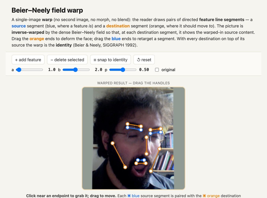
Some features are more naturally specified by lines than by points, such as an eyebrow, a jawline, or the edge of a roof. Feature-based field warping Beier & Neely lets the user draw pairs of directed line segments, before and after. For the backward lookup below, unprimed endpoints specify the destination segment and primed endpoints the source segment. Each segment pair sets up a local coordinate frame: a coordinate $u$ measured along the segment (normalized, $0$ at $\mathbf{P}$ and $1$ at $\mathbf{Q}$) and a coordinate $v$ measured perpendicular to it (in absolute distance units). For a single segment we inverse-warp: read a destination point $\mathbf{X}$'s coordinates $(u,v)$ in the destination frame and reconstruct the matching point in the source frame,
with $\perp(\cdot)$ the $90°$ rotation. A reported subtlety from the original work: $u$ scales with the segment (so a stretched feature carries its interior along) but $v$ is kept absolute. The authors tried scaling $v$ too and it looked worse. With multiple segments, each segment $i$ proposes its own displaced point $\mathbf{X}'_i$, and the final position is a distance-weighted average of those proposals, with weight
where $\ell_i$ is the segment's length (longer segments carry more authority), $d_i$ is the distance from the point to the segment (nearer segments dominate), and $a,b,p$ tune the falloff. This is the technique behind the morph in Michael Jackson's Black or White video and a perennial course project; it is built here and used in Chapter 11.3, Morphing (Figure 11.1.9).
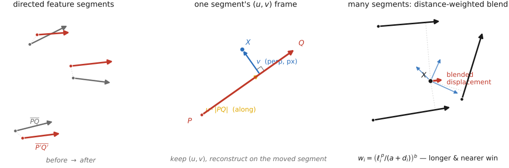
Figure 11.1.10 takes one output pixel through this computation, starting with a single segment.
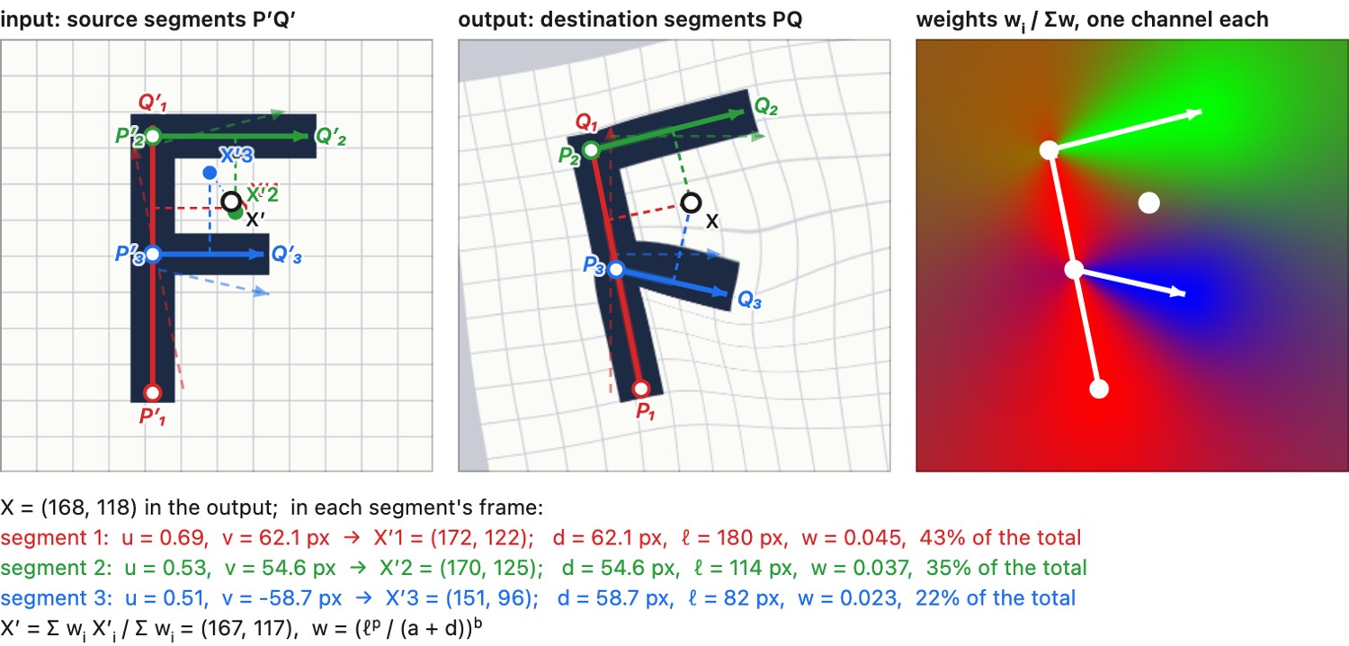
With two segments, each proposes its own source point and the warp averages them.
The weights form a field over the whole output.
Liquify: brush-driven warping⧉
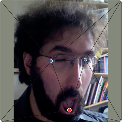
optionalEverything this chapter built, a dense map $f$ authored from sparse local input, then applied by resampling, is exactly what you are doing when you push pixels around with Photoshop's Liquify tool (the cosmetic "slim the waist / widen the smile" slider in spirit). Adobe does not publish the algorithm, but its documented behavior is the standard mesh warp. Under the hood Liquify keeps an editable mesh over the image, which you can show on screen and save to disk, and each brush stamps a smooth, radially-weighted displacement onto the mesh vertices beneath the cursor: Forward Warp pushes them along the drag, Twirl rotates them, Pucker and Bloat pull them in or out. The displacements accumulate as you stroke, Freeze masks pin regions you want protected, and Reconstruct relaxes the field back toward the identity. Because the brush specifies where pixels go, it authors the warp in the forward direction; the picture you see is that deformed grid resampled with interpolation. This is the forward-vs-inverse and reconstruction-filter machinery of this chapter, now driven by a paintbrush.
Face-aware deformation can use detected landmarks as semantic handles for eye, mouth or jaw adjustments. The detector and deformation model both affect the result; similar controls do not establish that different software uses an identical mesh algorithm.
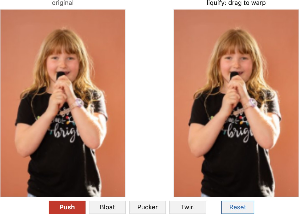
A deformation brush also makes the need for shape constraints visible. A position edit can bend a nearby architectural line or narrow a limb along with the intended feature. The operator must inspect the surrounding geometry, protect it with controls, or use a deformation model that penalizes the unwanted change. Chapter 11.5, Shape-preserving warping develops that last option.
Antialiasing for complex transforms⧉
When the footprint stops being a square: the warp Jacobian⧉
optionalRecall the engine. Inverse warping reads the source at $f^{-1}(x,y)$: for each output pixel, pull it back through the inverse map and look up the color there. But an output pixel is not a point. It is a little area, and what we owe it is the average of the source over the whole region that maps into it. Under a uniform scale that region is a square, the isotropic L16 kernel covers it exactly, and we are done. Under a general warp it is not a square, and the whole chapter follows from what shape it actually is.
Let $J=\partial f^{-1}/\partial(x,y)$, with output coordinates in pixels and mapped source coordinates in source pixels. A circular reference kernel transforms to an ellipse; a square pixel maps locally to a parallelogram. Thus the ellipse is a filter model, not the exact shape of every pixel. For a unit circular reference, the singular values of $J$ give its axis scales and the left singular vectors give source-space directions. More generally its covariance is $J\Sigma_{\rm out}J^\top$. EWA combines this with source reconstruction support; a common Gaussian model adds $\Sigma_{\rm recon}$. The ratio of singular values describes local anisotropy, not the absolute minification scale.
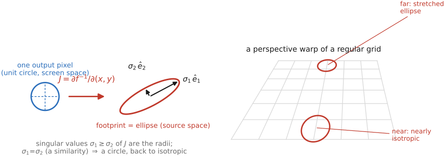
The canonical offender is exactly the floor we opened with: a checkerboard plane rendered in perspective, or rectified to perspective. Near the camera one pixel covers one tile and $\rho\approx1$; toward the horizon one pixel covers many tiles in depth but only one across, and $\rho$ climbs into the tens or hundreds. That is where every isotropic filter visibly fails, and the failure is not a matter of taste but of geometry. A round kernel has one radius, and the footprint has two very different ones. The fix is to make the kernel an ellipse that matches the footprint: the L16 prefilter, now carrying an orientation. Figure 11.2.2 shows the three outcomes side by side on a genuine perspective checkerboard.
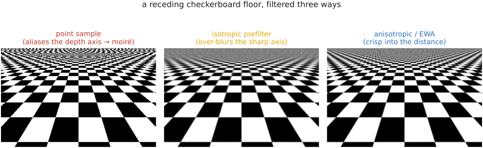
For example, suppose the inverse warp stretches one output-pixel distance into four source-pixel distances horizontally and one vertically. A circular source filter wide enough for the horizontal compression also averages too much vertically. A filter narrow enough to retain the vertical detail leaves horizontal frequencies that can alias. An elongated footprint expresses the two requirements separately. Rotate the warp and the long axis rotates as well; a scalar level-of-detail value cannot describe both its orientation and its unequal axis lengths. The ellipse is a convenient approximation based on a circular filter footprint and a local linearization, rather than the exact image of a square pixel under an arbitrary nonlinear warp.
Morphing⧉
PS5 implements a full Beier–Neely morph (warp + cross-dissolve). → Chapter 1.5, Problem sets (appendix).
Two photographs of two different faces, and the goal is a film clip that turns one into the other, not as a cut or a fade, but a single face that becomes another, the way the dancers shapeshift through each other at the end of Michael Jackson's Black or White. The obvious tool is the cross-dissolve: at each in-between time $t$, set every output pixel to the linear blend of the two inputs,
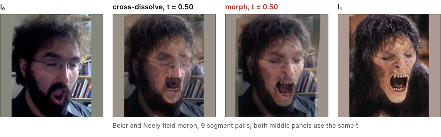
Run it and the result disappoints in one very specific way. Halfway through, at $t=0.5$, you do not see a plausible single face. You see a ghost: four faint eyes, two noses, a doubled mouth, all translucent and superimposed. The blend is doing exactly what you asked, averaging colors at fixed pixel locations, but the two faces' features sit at different pixels. The left image's left eye lands on the right image's eyebrow; the right image's mouth lands on the left image's chin. Averaging colors across that misalignment double-exposes every feature.
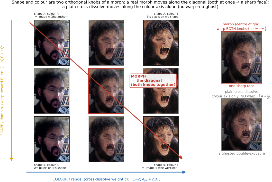
The diagnosis is sharp, and it is the whole chapter. A cross-dissolve interpolates only the range, the color at each location. To get a believable in-between you must also interpolate the domain, the location of every feature, so that both pairs of eyes travel to the same place before you average them. Metamorphosis is what you get when you do both: warp each image so its features move toward a common intermediate shape, then cross-dissolve the now-aligned images. The one idea to hold is the separation of shape and color: interpolate where things are and what color they are as two independent linear blends, applied together.
A morph uses correspondences to create an intermediate shape, warps both inputs into it, and blends their appearance. The correspondence model is what prevents doubled features; a color blend alone cannot do that.
A morph is a correspondence field plus transport, then a blend. To interpolate between two images you cannot average their colors where they sit; you must first establish a correspondence between their features, transport (warp) both images along that correspondence to a common intermediate shape, and only then blend. Separating the manipulation into a domain part (the warp: where features are) and a range part (the color blend: what they are), and interpolating each linearly, is what makes the in-between read as one object transforming rather than two pictures fighting. The same three-part shape (correspond, transport, blend) drives panorama de-ghosting, multi-frame super-resolution's sub-pixel alignment, and flow-driven frame interpolation; the only thing that changes is how the correspondence is obtained (here, sparse user lines; in Chapter 12.8, Optical flow, a dense automatic field).
Averaging two images only makes sense once their features sit at the same place. A plain cross-dissolve blends colors at fixed coordinates, so any misalignment double-exposes into a ghost; the cure is always to warp into correspondence first, then average. You have already met this move under other names: panorama de-ghosting registers overlapping frames before feathering them, and multi-frame super-resolution aligns sub-pixel-shifted shots before merging (cross-ref Chapter 20.3, Blending). Morphing takes the lesson to its limit: it interpolates the alignment itself smoothly over $t$, rather than aligning once. The dense, automatic aligner that makes this work without hand-drawn lines is Chapter 12.8, Optical flow.
Why a cross-dissolve isn't enough: the ghosting motivation⧉
The goal is to smoothly turn one image into another, where "smooth" carries a strong requirement: each in-between $I_t$ should look like a plausible single image, not a visible blend of two. A face becoming a face; one video keyframe becoming the next.
The naive attempt is cross-fading (a.k.a. cross-dissolve): linearly interpolate colors pixel by pixel, $\text{out}[y,x]=(1-t)\,I_0[y,x]+t\,I_1[y,x]$. This is the right idea for color (at $t=0$ you get $I_0$, at $t=1$ you get $I_1$, and the color glides linearly between), but it ignores position entirely.
It ghosts because the two images' features are not aligned: eyes, mouth, and silhouette sit at different pixels. Blending colors at fixed locations superimposes a left-image eye onto a right-image cheek, and the result is a translucent double exposure, four eyes, two mouths (Figure 11.3.1). And you generally cannot repair this with a single global alignment. Translating, rotating, or scaling one image as a whole can register a couple of features at the cost of the rest, because two faces differ locally and non-rigidly: the jaws are differently shaped, the eyes differently spaced. No one rigid motion brings all the features into register at once.
So cross-fading interpolates only the range (color). A believable in-between demands that we also interpolate the domain, the location of every feature, and that is a warp, the missing half. The plan for the rest of the chapter: get a dense shape interpolation from sparse correspondence, and combine it with the color interpolation we already have.
Two interpolations: domain (shape) and range (color)⧉
The cure has two knobs. Name them precisely, because the method is their product.
Range interpolation (color) is the cross-dissolve we already have: at a location $x$, blend the two colors,
a straight linear blend of pixel values.
Domain interpolation (location) treats a feature point as a vector and interpolates where it is. For a corresponding pair, a point $P$ in $I_0$ and the matching point $Q$ in $I_1$, the in-between location is
At $t=0$ the feature sits where $I_0$ put it; at $t=1$ where $I_1$ put it; in between it travels straight along the segment $PQ$ (Figure 11.3.2). This is interpolation of the domain, the coordinate grid itself, as opposed to the color living on it.
To realize a domain interpolation as an image operation we warp: move pixels spatially while leaving their colors alone, $C'(x,y) = C\big(f(x,y)\big)$. In practice we use the inverse / backward map (for each output pixel, look up where it came from, $\text{out}(x,y)=\text{im}\big(f^{-1}(x,y)\big)$), so every output pixel is filled (no holes) and resampling is well-defined. This is exactly the engine of Chapter 11.1, Warping; morphing is one of its biggest customers, calling it twice per frame (once for each source image).
The morph in one line: interpolate the domain like a vector, then interpolate the range (color). A morph is the product of a shape interpolation and a color interpolation: two independent linear blends, applied together (Figure 11.3.2).
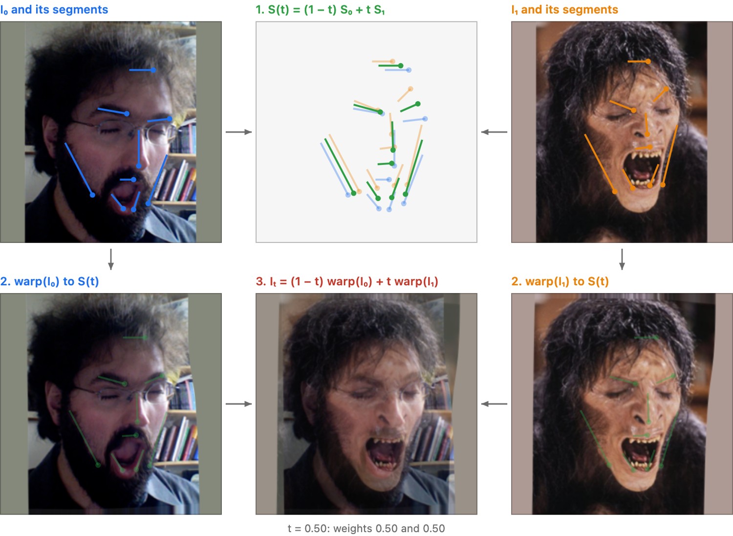
The morphing recipe (combine both)⧉
The inputs are the two images $I_0$ and $I_1$, plus sparse correspondences the user marks on both: matching line segments, or matching mesh vertices (which primitive is the next two sections). The output is a sequence of in-betweens $I_t$, $t\in(0,1)$. Each frame is built in four steps:
- Interpolate the feature geometry to an intermediate shape: each corresponding pair (point, segment, or vertex) goes to its in-between location $P_t=(1-t)\,P_0+t\,P_1$.
- Build two dense warp fields from the sparse pairs: one carrying $I_0$'s features onto the intermediate shape, the other carrying $I_1$'s features onto the same intermediate shape.
- Warp both images to that common shape. Now $I_0$ and $I_1$ are feature-aligned: both pairs of eyes land on the same pixels, both mouths coincide.
- Cross-dissolve the two warped images, $I_t=(1-t)\,\text{warp}(I_0)+t\,\text{warp}(I_1)$. Because they are now aligned, the blend is sharp, with no ghosting (Figure 11.3.3).
A natural question is why warp both images, not just one. You could warp $I_0$ all the way onto $I_1$'s shape and dissolve, but then features would slide the whole distance while colors merely faded, and the early and late frames would be badly over-distorted (one image stretched to fit the other's geometry while still wearing its own colors). Meeting in the middle, with both images warped only partway, to the shared intermediate shape, keeps each warp small and symmetric, and is what makes the motion read as a single object transforming rather than one picture deforming into another.
The recipe interpolates both shape and color, and the endpoints prove it. At $t=0$ the intermediate shape equals $I_0$'s own shape, so the warp of $I_0$ is the identity, and the color weight on $I_1$ is zero: the output is exactly $I_0$. Symmetrically at $t=1$ the output is exactly $I_1$. The morph passes cleanly through both originals.
One cross-reference closes the loop. The correspondences here are user-specified and sparse: a person draws a few lines or drags a few vertices. The automatic, dense way to obtain correspondence between two images is Chapter 12.8, Optical flow, and that is precisely what frame-interpolation and slow-motion methods use to morph between video frames without any hand-drawn lines (Chapter 30.4, Frame interpolation and slow-motion synthesis).
Write the two backward maps from intermediate coordinates to the inputs as $b_{0,t}$ and $b_{1,t}$. Then
The tildes indicate reconstruction and footprint filtering. For radiometric blending use a common linear-light representation; encoded-value blending gives a different transition. Use masks where one input is invalid or occluded. With meshes, share connectivity across both inputs and the intermediate shape, and reject zero-area or flipped triangles. Matching endpoints does not guarantee valid geometry at every intermediate time.
Field morphing: the Beier–Neely line-pair warp⧉
The first way to turn sparse correspondence into a dense warp is due to Beier and Neely (1992), whose Feature-Based Image Metamorphosis is the technique behind the Black or White video and a perennial problem-set favorite. The primitive is a pair of directed line segments, one drawn on the "before" image and one on the "after", declaring "this feature edge here corresponds to that feature edge there" (the jaw line, the bridge of the nose, the line of an eye). A handful of segments is enough; the warp interpolates everywhere between them.
The mechanics of that warp are built in full in Chapter 11.1, Warping, and we only recall them here. A before/after pair $\overline{PQ}\to\overline{P'Q'}$ sets up a segment-relative coordinate frame: a normalized coordinate $u$ along the supporting line, with $u=0$ and $u=1$ at the segment endpoints and a signed perpendicular distance $v$ in pixels, and a query point keeps its $(u,v)$ as it is reconstructed against the primed segment ($u$ scales with the segment's length, $v$ stays in absolute pixels). Several line pairs are reconciled by the distance- and length-weighted average of their proposed displacements, $w_i=(\operatorname{length}_i^{\,p}/(a+\operatorname{dist}_i))^{b}$ with the capped point-to-segment distance (cross-ref Figure 11.1.9 in Chapter 11.1, Warping, where the $(u,v)$ frame and the weight are derived). As always the map runs backward, $(u,v)$ is computed in the destination and looked up in the source, so every output pixel is filled.
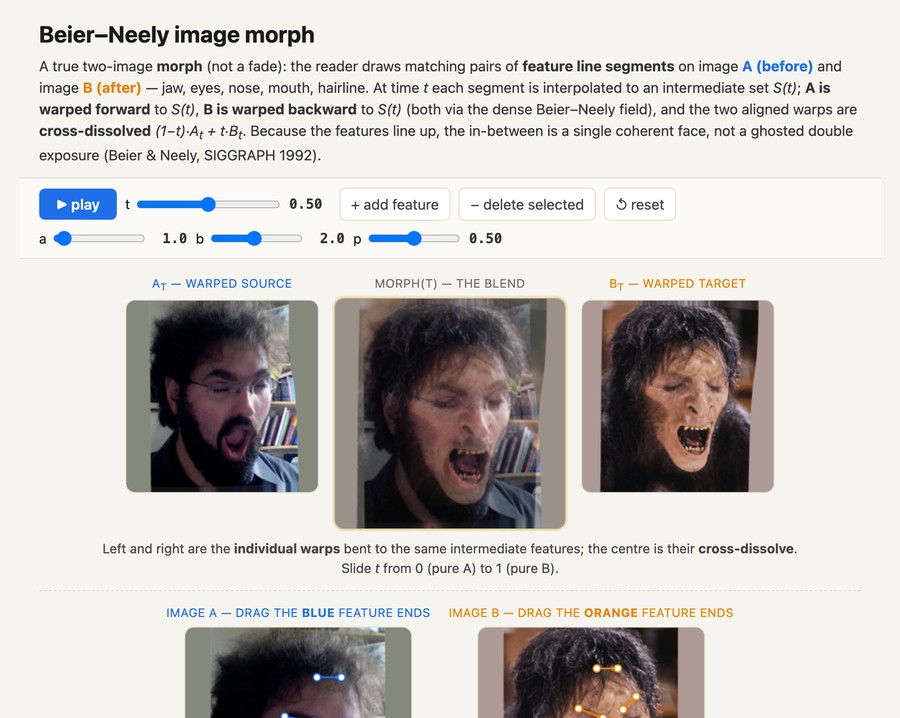
What matters for morphing is only how that warp is driven: at parameter $t$ the line pairs are interpolated to an intermediate set $\overline{P_tQ_t}=(1-t)\overline{PQ}+t\overline{P'Q'}$, and each source is warped to that shared intermediate geometry before the cross-dissolve. The same handful of feature lines thus does double duty, defining the dense field and, by their own interpolation, the in-between shape.
Strengths and weaknesses. The strength is sparse, intuitive control: draw a few feature lines and get a smooth field, with no mesh to manage. The weakness is that every line affects every pixel (global support, so each frame costs $O(\#\text{pixels}\times\#\text{lines})$) and far-apart lines can fight, producing "ghost" pulls and folds where their proposed displacements disagree; getting $a,b,p$ right and debugging the distance function are a real part of the work. Two practical bells and whistles: morph the foreground only (matte it first) so an unconstrained background does not drag artifacts into the result, and use non-uniform timing (let different features morph at different rates) for more lifelike transitions: a turning head might lead with the nose.
Mesh / triangulation morphing (the alternative warp)⧉
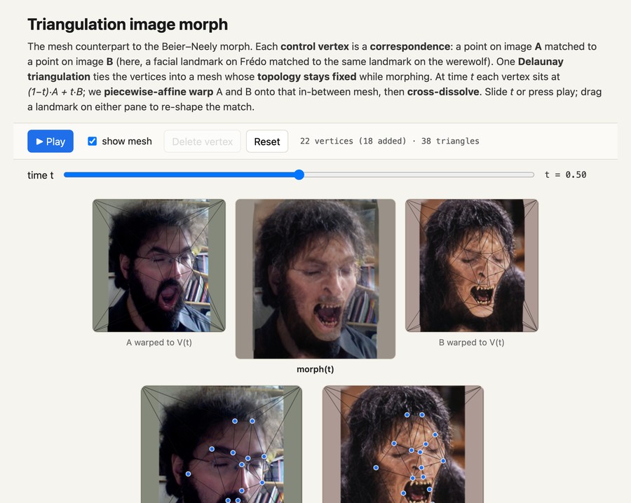
optionalThe second way to get a dense warp swaps lines for a mesh of corresponding control points placed on both images (or a regular grid deformed to match features). Triangulate the points; each triangle in $I_0$ corresponds to the matching triangle in $I_1$.
The warp is then trivially local: within each triangle the map is a single affine (barycentric) transform, which is fast to evaluate and invertible when both triangles have nonzero area. The intermediate shape is the mesh with its vertices interpolated to $P_t=(1-t)P_0+tP_1$; warp each source by its per-triangle affine onto that mesh, then cross-dissolve. Spline and free-form mesh variants (Wolberg's Digital Image Warping; multilevel free-form warps) trade the piecewise-affine creases at triangle edges for a smoother field.
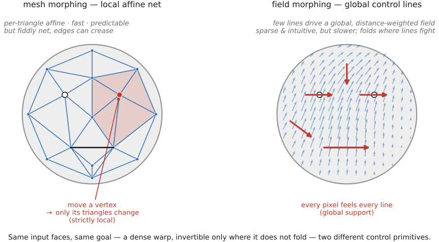
Field versus mesh, the trade-off (Figure 11.3.6). A mesh warp has local support: moving a vertex disturbs only its incident triangles, which makes it fast, predictable, and free of the far-line fights that plague field warps, but the control net is fiddly to author, and triangle edges can crease if the triangulation is poor. A field (Beier–Neely) warp has global, line-based control that is sparse and intuitive to draw, but it is slower and can fold. Same job: turn sparse correspondence into a dense warp, checking separately for folds and degeneracy, expressed in two different bases (a triangulation versus a set of influence lines).
Either way, the warp is a domain transform that must reconstruct and prefilter as it resamples (minified regions averaged down, magnified regions smoothly interpolated up), exactly the elliptical weighted average (EWA) Heckbert 1989 / mip machinery of Chapter 11.1, Warping. Because a morph stretches some regions hard while crushing others, it is a genuine stress test for good resampling: cut corners on the prefilter and the in-betweens alias and shimmer.
View morphing: the geometrically-correct in-between of two views⧉
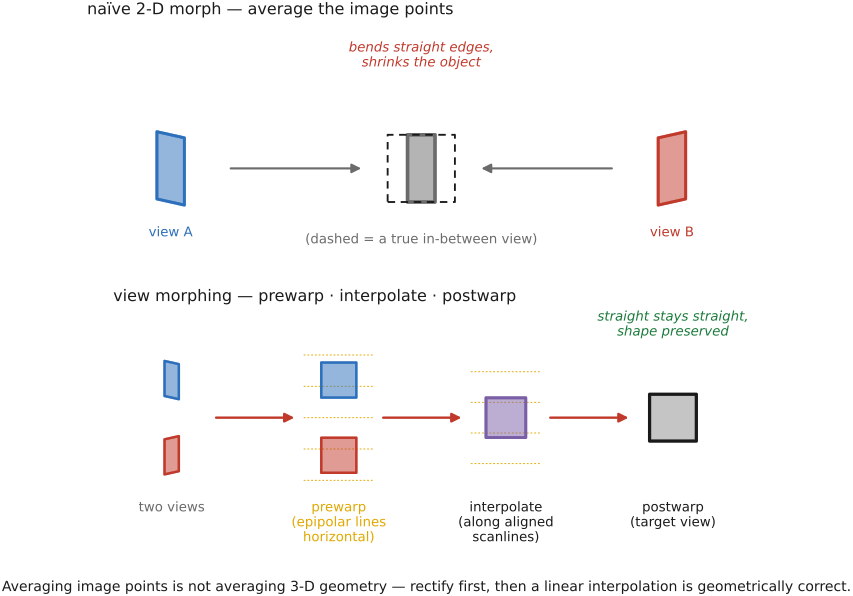
optionalThere is a case where the flat 2-D morph above is silently wrong. Suppose $I_0$ and $I_1$ are not two arbitrary pictures but two photographs of the same 3-D scene from different viewpoints, such as a face rotating between two camera angles. A naive linear morph then bends straight lines and shrinks the object: the in-between is not a valid view of any rigid scene (Figure 11.3.7). The reason is fundamental. Linearly interpolating image positions is not the same as interpolating the underlying 3-D geometry. A straight edge in the world projects to a straight line in both photos, but the midpoint of its two image projections is generally not where that edge would project from an in-between camera; the linear average cuts a chord across the true projective path, so straight lines sag and the silhouette pinches inward.
The fix, due to Seitz and Dyer (1996) in View Morphing, restores physical validity with three steps:
- Prewarp both images by homographies that rectify them to a common plane, so the two image planes become parallel and corresponding epipolar lines are horizontal and aligned (the same rectification used in stereo).
- Linearly interpolate the now-rectified images, a plain morph. But in this rectified frame the linear interpolation is geometrically correct, because corresponding points are constrained to move along aligned scanlines, so averaging their positions tracks the true motion.
- Postwarp the interpolated result by an interpolated homography to the desired in-between view.
Under rectified equal-intrinsic cameras translated parallel to their image planes, a fixed visible 3-D point moves linearly in image coordinates along the baseline. This is the special geometry exploited by view morphing Seitz & Dyer 1996. It does not imply that every camera motion admits a plain linear image blend. Correspondences, visibility and the pre/postwarps still determine whether the interpolated view is valid.
The connection outward is direct. View morphing needs corresponding points between the two views and the epipolar geometry relating them: exactly the correspondence problem of Chapter 12.8, Optical flow and stereo. Supply that correspondence densely and automatically and you can synthesize in-between views with no hand-drawn lines at all: the bridge from morphing to image-based rendering, and to flow-driven frame interpolation (Chapter 30.4, Frame interpolation and slow-motion synthesis), where the two "views" are simply adjacent video frames.
Recap and significance optional⧉
optionalThree ideas last past this chapter. First, interpolating color alone introduces blur and ghosts: a plausible in-between also interpolates position. Second, separate shape and color, interpolate each as its own blend, and recombine them. Third, non-rigid alignment of two different images is a reusable primitive: once you can warp one image into correspondence with another, you can interpolate between them, average them, exaggerate the difference, or re-render from a new viewpoint, within the range where the correspondence holds.
That last sentence is where morphing reaches into the rest of the book. The canonical face morph is only the showpiece. Video frame interpolation and slow-motion are morphing between adjacent frames (Chapter 30.4, Frame interpolation and slow-motion synthesis); MPEG-style motion prediction is morph-by-motion-field; morphable face models warp a mean face by shape parameters; and motion magnification (Liu et al. 2005) analyzes a motion field, magnifies it, and warps by the magnified field: a morph whose correspondence comes from motion analysis. The common thread is that everything here hinged on correspondence, which we obtained by hand. Getting that correspondence automatically and densely is the subject of Chapter 12.8, Optical flow, over in the matching-and-tracking part.
Morphable models⧉
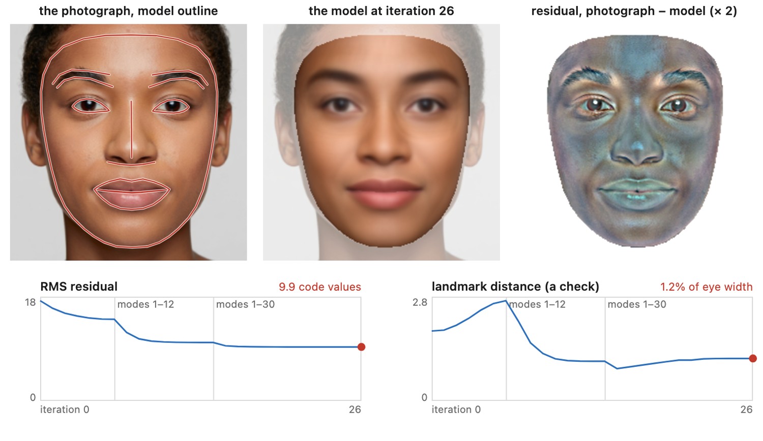
optionalA single linear morph turns one face into another by interpolating a hand-drawn correspondence: it knows about exactly two faces and the straight line between them. Suppose instead you have a hundred faces, all registered to one another, and you ask a bigger question: what does the space of all of them look like, and can I synthesize, recognize, or edit a face by navigating that space? That is the move from a morph to a morphable model, and it is one of the most influential ideas in this part: a whole family of shapes (faces, bodies, a class of objects) captured as a mean plus a basis of deformations, so that members can be approximated by low-dimensional coordinate vectors. The basis also represents implausible shapes; a prior and validity checks restrict how it is used.
The construction is short to state and is built from machinery you already own. Put a training set of examples into dense correspondence (every example's nose-tip maps to every other's), align away the nuisance pose with Procrustes, and take the principal components (PCA) of the aligned shapes. PCA hands back a mean shape and an ordered basis of eigen-deformations, the directions in which the family varies most, and any instance is written
the mean plus a weighted sum of eigen-modes, with coordinates $\mathbf{c}=(c_1,c_2,\dots)$ measured in units of each mode's standard deviation $\sigma_k$. Read in this part's language, $\bar{\mathbf{s}}$ is a mean shape and the $\mathbf{e}_k$ are a learned warp basis over it: each eigen-mode is a small canonical deformation of the mean, and an instance is the mean warped by a linear combination of them. A morphable model is morphing, with the correspondence field constrained to the subspace the data taught us is plausible (Figure 11.4.1).
The same idea recurs at three scales of fidelity, and they share one skeleton. In 2-D, Cootes, Edwards and Taylor's Active Shape / Active Appearance Models (ASM 1995 Cootes et al. 1995 (ASM), AAM 2001 Cootes et al. 2001 (AAM)) build PCA models of landmark shapes (and, for AAMs, of the shape-free texture too) and fit them to images. In 3-D, Blanz and Vetter's 3D Morphable Model of faces (1999) Blanz & Vetter 1999 is the landmark result: a PCA model of 3-D face geometry and texture, fit to a single photograph by analysis-by-synthesis to recover shape, albedo, pose, and lighting at once. The same recipe gives SMPL for human bodies (Loper et al. 2015) Loper et al. 2015 (SMPL) and FLAME for faces (Li et al. 2017) Li et al. 2017 (FLAME). Egger et al.'s 2020 survey Egger et al. 2020 is the map of the whole territory. We develop the skeleton once; the differences are scale (2-D vs 3-D), what gets a basis (shape, texture, expression), and how the prior is parameterized (linear PCA vs a neural net).
Everywhere in this part the recipe is build a coordinate map, then transport the pixels; what changes is how the map is obtained. A parametric warp solves it from constraints; a morph interpolates a hand-drawn one between two images; a morphable model learns the basis of maps from a training population and then lets you pick one by its coordinates. The mean shape is the origin, the eigen-deformations are the basis vectors, and an instance is a short vector $\mathbf{c}$ of how far to move along each. Folding correspondence into a learned basis rather than a per-pair drawing buys a prior: not every warp is allowed, only the ones the family actually exhibits, which is exactly what lets the model fill in an occluded cheek, reject an implausible fit, and generalize from one photo to a full 3-D face. The same shape, mean + learned basis of deformations + coordinates, underlies SMPL bodies, FLAME faces, and, at the end of the chapter, the latent spaces of generative networks. (L17 is registered in the part introduction, Warping and morphing; here the map is a statistical model rather than a drawn or estimated one.)
A morphable model is the family-constrained sibling of the per-pair morph of Chapter 11.3, Morphing; its fitting step is an inverse-rendering analysis-by-synthesis that anticipates monocular 3-D reconstruction in Part 36, 3D and depth; and its linear PCA prior is the classical ancestor of the neural image and shape priors in Chapter 7.3, Deep learning and Chapter 14.1, What can super-resolution actually do?. Downstream it powers identity-preserving portrait editing, relighting, and avatar animation.
Step 4: shape and appearance are separate bases⧉
optionalA face is a shape and also a coloring: skin tone, the dark of the brows and lips, shading. A morphable model handles these with two separate bases, and keeping them separate is exactly the separate-shape-from-color discipline of Chapter 11.3, Morphing, now applied to a whole family. Geometry gets the shape PCA above. Appearance (texture) gets its own PCA, but the textures are first warped to the mean shape so they are compared in a common, shape-free frame (every face's texture sampled at the same canonical landmarks before averaging). The result is a mean texture $\bar{\mathbf{t}}$ and an appearance basis $\mathbf{a}_k$, and a full instance is the pair
with two coordinate vectors: $\mathbf{c}$ for geometry and $\mathbf{b}$ for appearance. To render an instance you synthesize the texture in the shape-free frame, then warp it onto the synthesized shape (the warp engine of Chapter 11.1, Warping, the morphable model's biggest customer after morphing): texture-on-the-mean, deformed to the geometry the shape coordinates request (Figure 11.4.1). Why separate them? Because they describe different properties: a change in width need not change skin tone, and a smile is primarily a geometric change. Separate bases do not establish statistical independence, and because untangling them is what makes the model useful: relighting edits the appearance/shading without touching identity geometry; re-posing edits geometry without re-painting the texture; recognition can compare two faces in shape alone, robust to lighting. Active Appearance Models combine the two into a single joint appearance model; the 3DMM keeps shape, texture, and the imaging parameters (pose, illumination) explicit so each can be read off after fitting.
Step 6: once fitted, edit by moving in the space⧉
optionalFitting makes the model useful. Once a photo is reduced to a point $\mathbf{c}$ (plus appearance $\mathbf{b}$, pose, and lighting), every downstream operation is a move in the space. The learned coordinates provide useful directions for editing, but large steps or combinations unsupported by the training data can produce implausible faces. Re-pose / re-illuminate: change the explicit pose and lighting parameters and re-render, giving the same identity from a new angle or under new light, the bread and butter of 3DMM-based face manipulation. Interpolate / average: the straight line between two fitted points is a morph that never leaves the family. The correspondence is built into the basis, which avoids the misaligned-pixel averaging of a cross-dissolve, though an intermediate shape can still be implausible (this is the morph of Chapter 11.3, Morphing, with the correspondence supplied by the model rather than drawn). Edit semantically: add a multiple of a mode that correlates with an attribute (older, wider, more of a smile) to push the face along that attribute while holding the rest. Recognize: compare faces in the identity coordinates, where pose and lighting have been factored out, so the same person under different conditions lands at nearly the same point, the use that motivated much of the original work.
This last group surfaces the identity-vs-expression factorization. The geometry of a face is the identity (bone structure, who it is, roughly constant for a person) composed with an expression (smile, frown, blink: momentary). A flat shape PCA blends the two; the more capable models give them separate factors (FLAME, for instance, carries distinct identity, expression, and pose/jaw parameters) so you can swap one person's expression onto another's identity, or animate a fixed identity through expressions. SMPL does the analogous split for bodies: a shape space (the person's build) and a pose space (the skeleton's articulation), with pose-dependent deformations layered on. The general pattern is to parameterize the deformation in separate groups (identity, expression, pose) each its own little basis, which is the rigging artist's blendshapes with a statistical prior.
Recap and significance optional⧉
optionalThree ideas outlast the specific models. First, a class of shapes can be modeled as a low-dimensional space: corresponded, aligned and reduced by PCA, a family collapses to a mean plus a basis of eigen-deformations, and a member within the model's range becomes a short coordinate vector. Second, separate shape from appearance (and, further, identity from expression from pose): independent factors, each its own basis, recombined by warping texture onto geometry, the morphing discipline at population scale. Third, fit by analysis-by-synthesis with a prior: search for the coordinates that reproduce the image, regularized toward the model's plausible region, so it can fill in what a single photograph does not show. A linear basis is a modeling choice, not evidence that the population is Gaussian, and a point in the space is plausible only near the data it was built from.
Those three put the morphable model at a crossroads in the book. Backward, it is morphing constrained to a learned family (Chapter 11.3, Morphing) built on the warp engine (Chapter 11.1, Warping). Forward, its analysis-by-synthesis fitting is the template for monocular 3-D face and body reconstruction (Part 36, 3D and depth); its data-term-plus-prior objective is the classical face of the regularized inverse problems that recur in Chapter 14.1, What can super-resolution actually do?; and its linear basis is the ancestor of the neural priors and generative latent spaces of Chapter 7.3, Deep learning, the same idea, a learned space of deformations over a mean, scaled up. The same pattern holds to the end: find the coordinate map, then move the pixels. Only here the map is learned from a population, and moving through it is how you synthesize, recognize, and edit an entire visual class.
Frame interpolation and slow-motion synthesis⧉
Interpolation = morphing between adjacent frames⧉
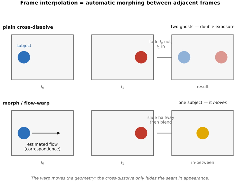
optionalThe cleanest way to understand frame interpolation is to recognize it as something you have already built. Chapter 11.3, Morphing takes two images plus a correspondence between them and produces in-betweens by warping both toward an intermediate shape and cross-dissolving. Frame interpolation is precisely that, with two consecutive video frames standing in for the two faces (Figure 30.4.2). The two endpoints, the warp-to-the-middle, the blend; all identical.
What changes is where the correspondence comes from. In classic morphing a human supplies it, drawing Beier–Neely feature lines from one image to the other by hand. In frame interpolation the correspondence is the optical flow, estimated automatically between the two frames. So the whole chapter reduces to one substitution. Frame interpolation is automatic morphing between adjacent frames: motion estimation replaces the hand-drawn correspondence.
Everything that makes interpolation hard, and everything the learned methods buy, lives in that one substitution: the correspondence is no longer given, it must be recovered, and it is recovered imperfectly.
This also explains, in one stroke, why you cannot skip the warp. A plain temporal cross-dissolve (fade frame $A$ out while frame $B$ fades in, with no warp) does not show an object moving; it shows two ghosts of the object, one at each position, the first dimming as the second brightens (Figure 30.4.2). The eye reads this as a double exposure, not as motion. The warp is exactly what collapses those two ghosts into one object that slides from $A$'s position to $B$'s. Morphing's lesson, restated for video: the cross-dissolve hides the seam in appearance, but only the warp moves the geometry, and motion is geometry.
Flow-based interpolation: warp both frames to the midpoint and blend⧉
optionalTake the morphing recipe literally and you get the classical, flow-based interpolator. Start from the assumption that between two close frames a pixel moves along a roughly straight, constant-velocity path. Then to synthesize the frame at fraction $t\in(0,1)$:
- Estimate flow both ways between the frames: $\mathbf{F}_{0\to1}$ (where each pixel of $I_0$ goes in $I_1$) and $\mathbf{F}_{1\to0}$ (the reverse).
- Map source locations toward time $t$ along scaled forward trajectories: frame $0$ is dragged a fraction $t$ of the way toward frame $1$, and frame $1$ a fraction $1-t$ of the way back toward frame $0$.
- Blend the two warped images, weighted by temporal closeness: a frame near $t=0$ should look mostly like $I_0$, one near $t=1$ mostly like $I_1$.
Written out, the synthesized frame is a convex blend of two backward-warped sources (Figure 30.4.3):
Here $\mathbf F_{t\to0}$ and $\mathbf F_{t\to1}$ are backward sampling displacements defined on the intermediate output grid, not simply the endpoint flow fields evaluated at the same coordinates. Read it back: for each output pixel $\mathbf{p}$, look back along the flow to where it sat in each real frame, sample the color there, and mix the two by how close $t$ is to each frame. The straight-line assumption is what lets us scale the flow vectors by $t$: we slide each pixel a fraction of the way along the one displacement we estimated.
Video compression and motion compensation⧉
optionalThe still-image part of this book taught one compression idea over and over: don't store what the viewer won't miss, and don't store what you can predict. JPEG (Chapter 8.11, File formats and compression) commonly subsamples chroma and quantizes transform coefficients, often more coarsely at high frequencies where errors can be less visible. Video adds a second, far larger redundancy that stills cannot touch: the next frame looks almost exactly like this one. At 30–60 frames per second the camera and the world barely move between frames; most of the picture is already on screen. Coding each frame independently (so-called Motion-JPEG, literally JPEG per frame) ignores this entirely and is wildly wasteful. Inter-frame codecs exploit prediction from decoded references and code residuals along with the information needed to construct that prediction. That is the whole subject.
Correspondence on a budget: motion compensation is optical flow you can afford. A codec needs, for every block, the same thing Chapter 12.8, Optical flow asks (where did this come from in a frame we already have?), but it does not need a physically correct, dense, sub-pixel flow field. It needs a coarse, block-constant correspondence field that is cheap to estimate and, above all, cheap to transmit, and it chooses that field to minimize total bits, not endpoint error. So decades before learned optical flow, video codecs were already estimating dense-ish correspondence at massive scale, optimized for rate, not accuracy. The recurring move: reuse what the decoder already has, and code only the difference. It returns inverted in Chapter 38.3, Motion and video magnification, which keeps the temporal difference instead of discarding it, and it is the rate-aware cousin of the correspondence story in Chapter 12.8, Optical flow.
Why video compresses far better than still × N: temporal redundancy⧉
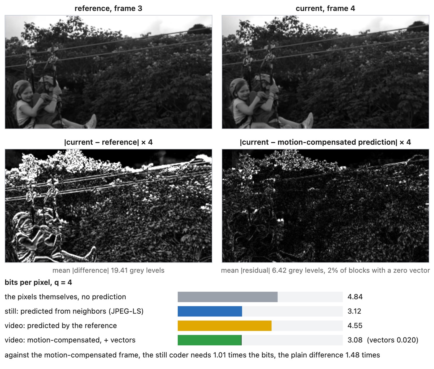
optionalHere is the single observation the chapter stands on. Take two consecutive frames of a camera on a tripod and subtract one from the other. The difference image $I_t - I_{t-1}$ is near-zero almost everywhere, black except at moving edges, occlusions, and lighting changes. That near-black difference image is the only new information the second frame carries; everything else was already on screen and need not be sent again (Figure 30.2.2). Measured on real clips, coding a tripod clip losslessly takes 3.1 bits per pixel frame by frame and 0.8 as frame differences. When the camera moves, the plain difference stops working: on a clip with real camera motion it takes 4.5 bits per pixel against 4.9 for the frame alone, and with a pan of 1.5 pixels a frame added it costs more than the frame alone on every clip. Compensating for the motion first brings it back down, to 4.05 bits per pixel on the moving clip, for about 0.01 bit per pixel spent on the motion vectors. That is the rest of this chapter.
The naive baseline ignores this. Motion-JPEG codes every frame as an independent JPEG: simple, edit-friendly, randomly accessible at any frame, but it pays the full still-image cost $N$ times and exploits none of the temporal redundancy. It is the "still $\times\,N$" strawman, and inter-frame coding can be much more efficient, with the gain depending strongly on content, quality, and codec settings.
The lever is to stop coding the frame and start coding the surprise. Instead of coding $I_t$, code the residual between $I_t$ and a prediction $\hat I_t$ assembled from already-decoded frames. If the prediction is good the residual is mostly zero, so after the DCT and quantization almost all coefficients vanish, and entropy coding then crushes a block that is nearly all zeros into almost nothing. The slogan is good prediction $=$ small residual $=$ few bits.
Two redundancies are now stacked. Video keeps JPEG's spatial and perceptual redundancy removal (the DCT, chroma subsampling, perceptual quantization, adapted from the same ideas as Chapter 8.11, File formats and compression, with codec-specific transforms and coding tools) and adds temporal redundancy removal on top. The temporal one is the large win.
The only question left is how to build $\hat I_t$. The crude answer, predict $I_t$ by the previous frame $I_{t-1}$ and code $I_t - I_{t-1}$, works when nothing moves but fails the moment anything does: a moving sharp edge sits in a different place in the two frames, so the difference lights up as a bright residual band exactly along every edge, precisely where coding is expensive. The fix is to predict with motion: line each block up with where it actually went, so the residual stays small even as the scene moves. That is motion compensation.
Motion-compensated prediction: the core trick⧉
optionalThe idea is geometric and simple. A moving object's block in frame $t$ is, to first order, the same pixels as some block in a reference frame, merely displaced. So for each block we find that displacement, copy the matched patch from the reference as our prediction, and code only what is left over.
The crude delta encoding above (code $I_t - I_{t-1}$, the difference at each fixed pixel) is Eulerian: it watches a stationary grid and asks what changed here. That is exactly why it collapses under motion: a moving edge changes the value at every pixel it sweeps past, so the Eulerian difference lights up everywhere there is movement, precisely where coding is expensive. Motion compensation is the Lagrangian fix: instead of differencing at a fixed location, it follows the content: find where each block went, displace the reference to meet it, and code only the small residual. The whole MPEG / H.264 family is Lagrangian video coding, and it beats Eulerian delta coding for the same reason warping beats per-pixel editing when things move: when the world moves, move with it. (Callback to L29, the Eulerian/Lagrangian split introduced in warping part.)
Macroblocks. Partition the frame into blocks, classically $16\times 16$ luma "macroblocks," though modern codecs use variable sizes down to $4\times 4$. Each block is predicted independently, with its own motion.
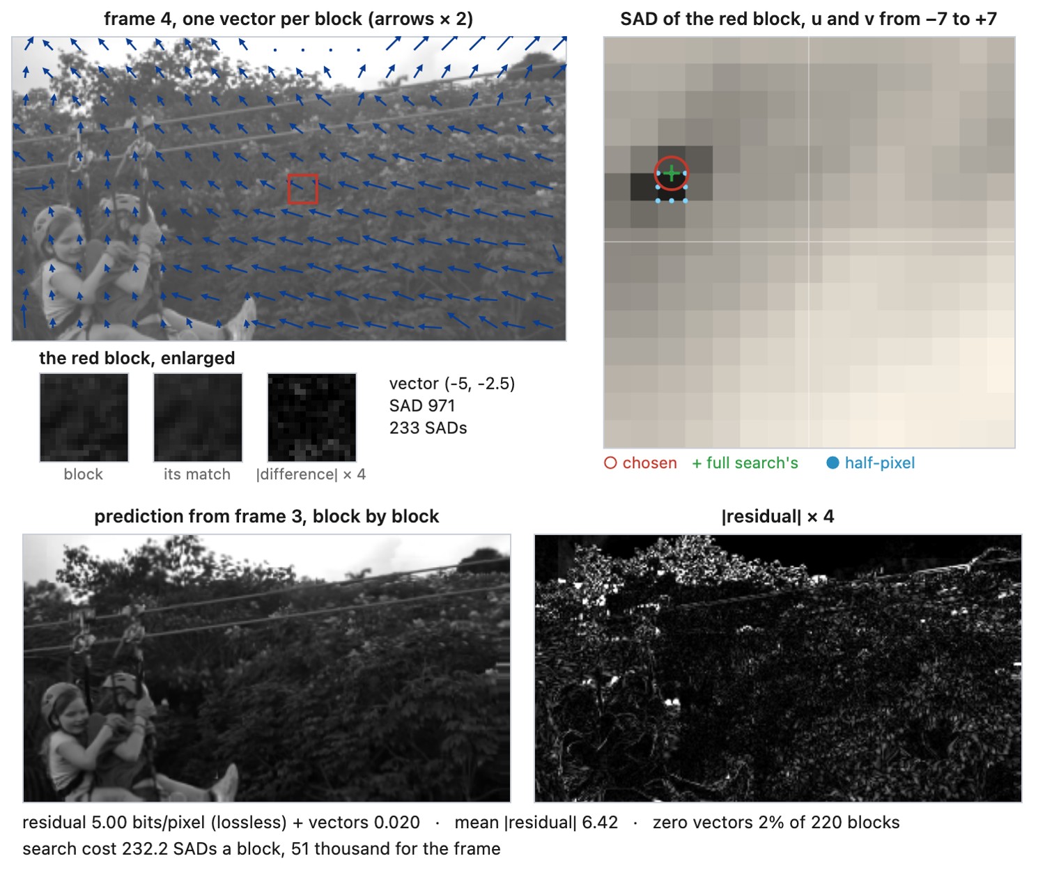
Block matching is the correspondence step, and it is exactly the cost-volume search of Chapter 12.8, Optical flow run per block. For a block $B$ in frame $t$, search a window in the reference frame for the best-matching patch and record the offset $(u,v)$, the motion vector:
This cost is the sum of absolute differences (SAD); the sum of squared differences (SSD) is its smooth cousin; the same matching primitive as Chapter 12.8, Optical flow, just summed over a whole block instead of a single pixel's neighborhood. Per block, it is a search over the displacement window for the cheapest match:
for each block B in frame I_t:
    best = ∞
    for (u, v) in search window:
        sad = ∑_{(x,y) in B} |I_t[x, y] - I_ref[x-u, y-v]|
        if sad < best:
            best = sad
            mv[B] = (u, v)
    residual[B] = B - I_ref shifted by mv[B]
The search is sped up with hierarchical, coarse-to-fine search and with predicted starting points from neighboring blocks, and sub-pixel motion vectors (half- or quarter-pel, found by interpolating the reference) sharpen the match further. Figure 30.2.3 runs this search on real video.
The prediction is then just the reference frame shifted by that vector,
and the residual, the thing we actually code, is what the prediction missed,
small wherever the match was good.
Transform-code the residual. Apply a codec-defined transform, quantize its coefficients under the chosen quality or quantization-parameter setting, and entropy-code them. This follows the transform/quantize/code pattern of Chapter 8.11, File formats and compression, but modern codecs need not use JPEG’s transform sizes, tables, or entropy coder. The codec transmits, per block, prediction-mode and reference information, motion information, and a coded residual where needed. Skip and merge modes can infer some of these rather than sending them explicitly. (The motion vectors are themselves predictively coded from their neighbors, since they too are spatially correlated; adjacent blocks tend to move together.)
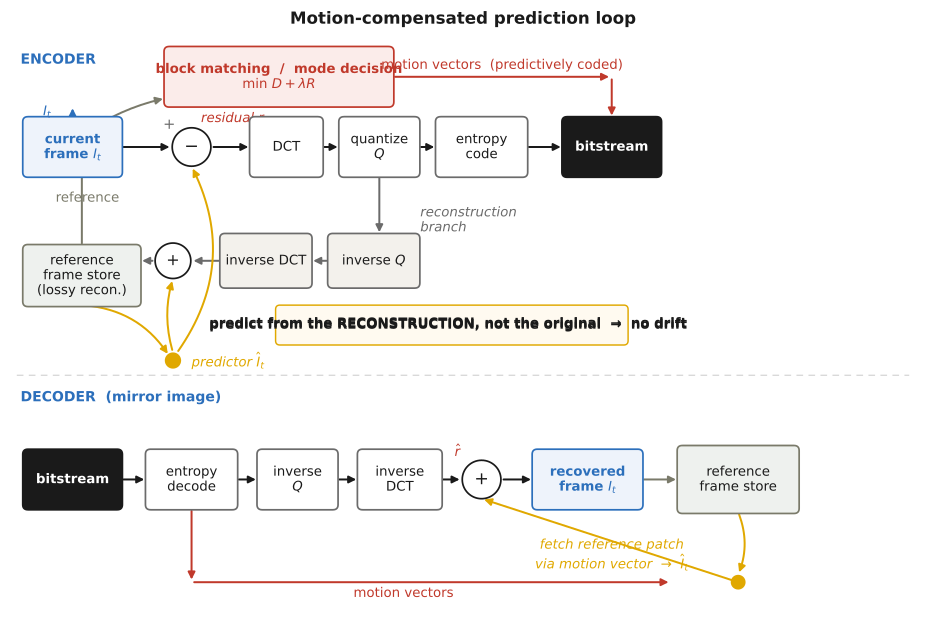
The decoder mirrors the encoder. It decodes the residual, fetches the same reference patch via the transmitted motion vector, and adds them: $\tilde I_t = \hat I_t + \tilde r$. Here tildes denote decoded quantities, including quantization error. One subtlety keeps the two sides in lock-step: the encoder predicts from the reconstructed (lossy) reference the decoder will actually have, not from the pristine original. If it predicted from the original, the small quantization errors would compound frame after frame and the two sides would slowly drift apart; predicting from the reconstruction makes encoder and decoder see the same reference and eliminates drift.
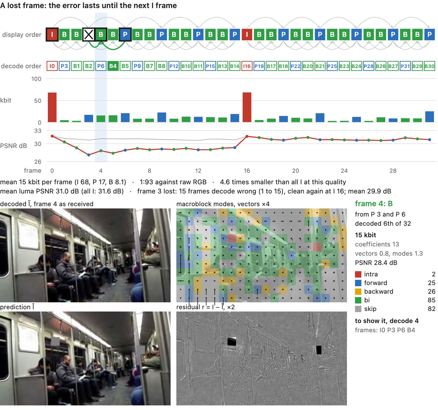
Figure 30.2.1 runs this loop on real video.
I P P P …, a GOP of 16). Each 16 × 16 macroblock of a P frame is predicted from the previous decoded frame by a half-pel motion vector $(u,v)$ found by block matching, and the encoder picks per macroblock whichever of skip (the predicted vector, no residual, one bit), a coded residual $r = I_t - \hat I_t$, or intra coding minimizes $D + \lambda R$. The lower panels show the prediction $\hat I_t$ and the residual (gray is zero, contrast doubled); the mode map colors each macroblock by its choice and draws its vector four times longer. On the subway clip, shaken by the train, a P frame costs about a fifth of an I frame; on the guitar and the sleeping baby nearly every macroblock is skipped and a P frame costs under 1 kbit against 53 to 81 kbit for an I frame. On the zipline, where the camera pans through foliage, a P frame still costs about 60% of an I frame (36 against 59 kbit) and a sixth of its macroblocks are coded intra, a third on the bear in rapids. An intra macroblock's prediction is flat gray, so its residual is the picture itself. Click a column to inspect a frame. Clips from Eulerian Video Magnification Wu et al. 2012, and the zipline and the bear in rapids, the author's.Rate–distortion is the real objective. The encoder does not pick the most accurate motion vector. It picks the one that minimizes
the reconstruction distortion $D$ plus $\lambda$ times the bits $R$ needed to send the vector and its residual. A slightly worse match that codes far cheaper wins outright. This $\min D + \lambda R$ trade-off is the same Lagrangian balance that sets a quantization table's aggressiveness in Chapter 8.11, File formats and compression. It is why the motion field is on a budget: it is optimized for bits, not for physical correctness (Figure 30.2.4).
I, P, and B frames; GOP structure⧉
optionalNot every frame can be predicted from another. You need an entry point with no dependency, and you would like to predict from both directions when you can. Codecs therefore define three frame types, and a frame's type is exactly its place in the prediction graph (Figure 30.2.1).
- I-frame (Intra). Uses intra coding without temporal prediction. Modern intra coding can predict blocks from spatial neighbors before transforming residuals. An intra picture alone does not necessarily reset later reference dependencies; formats distinguish random-access refresh pictures such as H.264 IDR pictures.
- P-frame (Predicted). Allows prediction from a reference list of decoded pictures, plus intra-coded blocks where useful. In a simple chronological GOP these references are earlier frames. Its size depends on content and encoder choices.
- B-frame (Bidirectional). Allows two prediction lists and combinations of predictions. A common case uses a past and a future frame, but modern reference structures are more flexible and a B picture need not use both temporal directions. Bidirectional prediction can reduce residuals, without guaranteeing the smallest frame size. The price is out-of-order decoding: the future reference must already be decoded, so a codec's coding order differs from its display order.
I B B P B B P …). A B frame predicts each macroblock from the anchor before it, the anchor after it, or the average of the two, and no frame is predicted from it. Arrows above the timeline are P-frame references, arrows below are B-frame references, heavy for the selected frame. Because a B frame needs its future anchor, the decode-order row sends each P frame before the B frames that precede it on screen. On the subway clip a B frame costs about half a P frame, the P frames, now three frames from their reference, cost more than with I P P P, and the sequence comes out about 10% smaller overall. On the nearly static clips at high quality the trade reverses: P frames were almost free already, and spacing them three apart costs more than the B frames save. On the zipline and the bear in rapids B frames do not pay either: I B B P comes out 3 to 7% larger than I P P P.GOP (Group of Pictures). The repeating arrangement of these types (for example I B B P B B P …, restarting at the next I-frame) is the GOP, and its length is a direct trade-off:
- short GOP (frequent I-frames) → easy random access and seeking, robust to errors, but bigger files;
- long GOP (rare I-frames) → best compression, but slow seeking and error propagation that lasts until a suitable refresh or recovery point clears the affected dependencies.
In practice streaming and editing favor shorter GOPs (you seek and splice constantly); archival and broadcast push longer GOPs for size. All-intra (I-only) modes also exist, for editing-friendly, frame-accurate video at the cost of size, which is essentially Motion-JPEG with a better intra coder.
Why this is "optical flow on a budget"⧉
optionalState the equivalence plainly, because it is the whole reason this chapter lives next to Chapter 12.8, Optical flow. The field of motion vectors over all the blocks of a frame is a correspondence field: a piecewise-constant, one-vector-per-block approximation to the optical flow between the frame and its reference. Block motion compensation supplies a prediction correspondence field, computed at scale in inter-frame codecs (Figure 30.2.5).
But it is the budget version, and the differences are the point.
- Block-constant, not per-pixel. One vector covers a whole block, even though the true flow varies within it. The residual absorbs the within-block error. The codec does not need the flow to be right, only cheap, because whatever it gets wrong is paid for once, in residual bits.
- Rate-optimal, not accuracy-optimal. The vector is chosen to minimize bits ($D + \lambda R$), so the encoder will happily pick a physically wrong vector when it codes cheaper. A codec's motion field is not a measurement of scene motion; do not read it as ground-truth flow.
- Block-matching, not variational. A simple encoder uses SAD/SSD search, related to Chapter 12.8, Optical flow, without a global smoothness solve. Actual encoders use varied search and mode-decision strategies; the bitstream standard specifies decoding rather than one required search algorithm. What smoothness there is comes implicitly, from predictively coding the vectors and from the rate cost of disagreeing with neighbors.
- Graceful fallback. When prediction is hopeless, as in a scene cut, fast new content, or a large occlusion, the encoder simply codes the block, or the whole frame, intra, degrading gracefully back to the still-image path.
The conceptual bridge runs both ways. The same aperture problem, search window, and sub-pixel interpolation appear in the codec and in flow estimation. Learned optical flow (RAFT and its kin, Teed & Deng 2020; see Chapter 12.8, Optical flow) and learned video codecs both build on this cost-volume correspondence skeleton; the codec just got there first, optimized for a different loss.
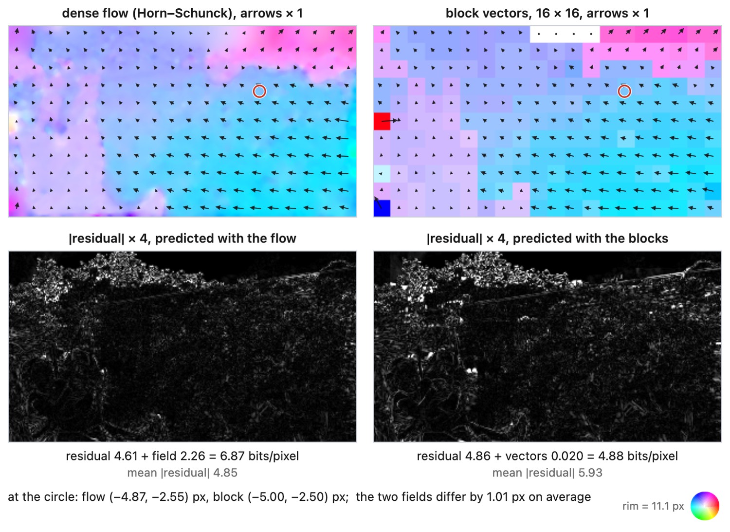
The flip side of "graceful fallback" is a failure mode you have certainly seen: when the motion is genuinely unpredictable, as in falling snow, confetti, churning water, or a field of static, there is no good block match anywhere, the residual balloons, and at a fixed bitrate the whole frame smears into mush. It is the most vivid everyday demonstration that video compression depends strongly on predictability, and Tom Scott's popular explainer makes exactly this point (Figure 30.2.6).
Modern codecs in one breath⧉
optionalThe lineage is long and the skeleton never changes: Moving Picture Experts Group (MPEG)-1/2 Le Gall 1991 (MPEG) → H.264 / Advanced Video Coding (AVC) (Wiegand, Sullivan, Bjøntegaard and Luthra 2003) → H.265 / High Efficiency Video Coding (HEVC) (Sullivan, Ohm, Han and Wiegand 2012) → AV1 (AOMedia Video 1; AOMedia, 2018) Chen et al. 2018 (AV1) → H.266 / Versatile Video Coding (VVC). Every one of them keeps the same three pieces: motion-compensated block prediction $+$ transform-coded residual $+$ entropy coding. What changes generation to generation is how each piece is implemented, not the architecture.
What they add, on the same bones:
- Variable / recursive block sizes: big blocks for flat, uniform motion, tiny blocks for fine detail, chosen per region.
- Multiple reference frames and better sub-pixel interpolation, so a block can be predicted from whichever past (or future) frame matches best.
- Intra prediction within a frame: predict a block from its already-decoded spatial neighbors using directional modes, so that even I-frames now beat a plain JPEG.
- Richer entropy coders such as CABAC (context-adaptive binary arithmetic coding).
- In-loop deblocking and sample-adaptive filters to hide the block edges that motion compensation and block-transform coding would otherwise leave.
- AV1 additionally brings warped / affine motion (a deliberate step toward true flow), overlapped-block motion compensation, and the practical advantage of being royalty-free.
Decades of codec progress is better prediction plus smarter residual coding inside an unchanged motion-compensation framework, and that framework is correspondence chosen under a bitrate constraint, applied to the temporal axis. Many learned codecs also exploit temporal prediction, but some code conditional latent representations rather than an explicit pixel residual. Predictive block coding explains the major conventional codec families; it is not a definition that covers every possible video representation.
Recap: big lessons in this lecture
Almost every geometric algorithm in the book has the same two-part shape: first establish a coordinate map between two images (or between an image and a target frame), then transport the pixels along it. This part builds that machinery and its first uses: warping makes the map explicit and applies it, perspective rectification solves the map (a homography) from geometric constraints, and morphing interpolates between two maps. The same shape recurs across the book: panorama stitching estimates the map from matched features (in the multiple-exposure part), optical flow estimates a dense map from brightness constancy (in the matching part), and stabilization smooths a map over time while frame interpolation renders along one (in the video part). Separating the two halves, what the map is versus how you transport pixels through it, is what lets one transport engine (inverse warp + resample, built in the next two sections) serve this part and recur throughout the book; only the map changes from task to task. (L17 is registered in the part introduction, Warping and morphing; this chapter is the transport engine, and the chapters that follow are different ways of finding the map.)
A morph is a correspondence field plus transport, then a blend. To interpolate between two images you cannot average their colors where they sit; you must first establish a correspondence between their features, transport (warp) both images along that correspondence to a common intermediate shape, and only then blend. Separating the manipulation into a domain part (the warp: where features are) and a range part (the color blend: what they are), and interpolating each linearly, is what makes the in-between read as one object transforming rather than two pictures fighting. The same three-part shape (correspond, transport, blend) drives panorama de-ghosting, multi-frame super-resolution's sub-pixel alignment, and flow-driven frame interpolation; the only thing that changes is how the correspondence is obtained (here, sparse user lines; in Chapter 12.8, Optical flow, a dense automatic field).
Averaging two images only makes sense once their features sit at the same place. A plain cross-dissolve blends colors at fixed coordinates, so any misalignment double-exposes into a ghost; the cure is always to warp into correspondence first, then average. You have already met this move under other names: panorama de-ghosting registers overlapping frames before feathering them, and multi-frame super-resolution aligns sub-pixel-shifted shots before merging (cross-ref Chapter 20.3, Blending). Morphing takes the lesson to its limit: it interpolates the alignment itself smoothly over $t$, rather than aligning once. The dense, automatic aligner that makes this work without hand-drawn lines is Chapter 12.8, Optical flow.
Everywhere in this part the recipe is build a coordinate map, then transport the pixels; what changes is how the map is obtained. A parametric warp solves it from constraints; a morph interpolates a hand-drawn one between two images; a morphable model learns the basis of maps from a training population and then lets you pick one by its coordinates. The mean shape is the origin, the eigen-deformations are the basis vectors, and an instance is a short vector $\mathbf{c}$ of how far to move along each. Folding correspondence into a learned basis rather than a per-pair drawing buys a prior: not every warp is allowed, only the ones the family actually exhibits, which is exactly what lets the model fill in an occluded cheek, reject an implausible fit, and generalize from one photo to a full 3-D face. The same shape, mean + learned basis of deformations + coordinates, underlies SMPL bodies, FLAME faces, and, at the end of the chapter, the latent spaces of generative networks. (L17 is registered in the part introduction, Warping and morphing; here the map is a statistical model rather than a drawn or estimated one.)
Correspondence on a budget: motion compensation is optical flow you can afford. A codec needs, for every block, the same thing Chapter 12.8, Optical flow asks (where did this come from in a frame we already have?), but it does not need a physically correct, dense, sub-pixel flow field. It needs a coarse, block-constant correspondence field that is cheap to estimate and, above all, cheap to transmit, and it chooses that field to minimize total bits, not endpoint error. So decades before learned optical flow, video codecs were already estimating dense-ish correspondence at massive scale, optimized for rate, not accuracy. The recurring move: reuse what the decoder already has, and code only the difference. It returns inverted in Chapter 38.3, Motion and video magnification, which keeps the temporal difference instead of discarding it, and it is the rate-aware cousin of the correspondence story in Chapter 12.8, Optical flow.
The crude delta encoding above (code $I_t - I_{t-1}$, the difference at each fixed pixel) is Eulerian: it watches a stationary grid and asks what changed here. That is exactly why it collapses under motion: a moving edge changes the value at every pixel it sweeps past, so the Eulerian difference lights up everywhere there is movement, precisely where coding is expensive. Motion compensation is the Lagrangian fix: instead of differencing at a fixed location, it follows the content: find where each block went, displace the reference to meet it, and code only the small residual. The whole MPEG / H.264 family is Lagrangian video coding, and it beats Eulerian delta coding for the same reason warping beats per-pixel editing when things move: when the world moves, move with it. (Callback to L29, the Eulerian/Lagrangian split introduced in warping part.)