Lecture Notes 3 — Noise, bilateral filter⧉
Course notes cut from Computational Photography, an AI-powered Slopendium for this lecture. Each section links back to its home in the book; sections marked optional go beyond what the lecture needs.
Contents · 17 sections on this page, from 10 chapters of the book
Titles jump to the section below; ↗ opens it in the book.
Noise, signal-to-noise ratio and dynamic range⧉
Signal-to-noise ratio: it's about ratios⧉
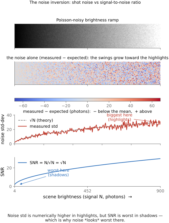
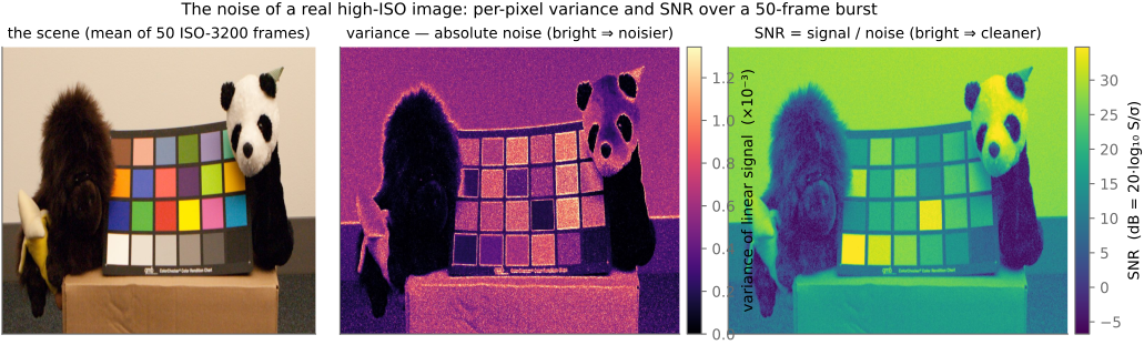
optionalA counterintuitive fact ties the whole part together. Since shot noise is $\sigma = \sqrt{N}$, the absolute noise is actually larger in the bright parts of the image than in the dark parts: a highlight collecting 10,000 photons has $\sigma = 100$, while a shadow collecting 100 photons has only $\sigma = 10$. And yet noise looks worst in the shadows. The resolution is that noise visibility depends strongly on its size relative to the local signal, as well as on display brightness, spatial frequency, and image content. Signal-to-noise ratio (SNR) captures the first of these effects. For shot noise,
The SNR grows with brightness, so it is worst where the light is faintest (the shadows) even though the raw noise magnitude is smallest there (Figure 2.8.6). This emphasis on ratios also motivates gamma and log encoding (log encoding gives equal steps to equal ratios, while a power-law gamma curve approximates perceptual spacing over a useful range) and exactly why exposing to the right works: collecting more photons everywhere, especially in the shadows, raises $N$ and therefore raises the SNR where it is worst.
One caution before we go on, because the acronyms collide: SNR is not PSNR. The signal-to-noise ratio here is a property of a capture, the true signal at a pixel relative to the sensor's noise there ($\sqrt N$ for shot noise), and it answers how clean is this measurement? Peak signal-to-noise ratio (PSNR), which you meet whenever an algorithm is evaluated, is a different animal: a full-reference quality metric that compares a processed image $\hat I$ against a ground-truth reference $I$, computed from their mean-squared error as
where $\mathrm{peak}$ is the largest possible value (e.g. often 1.0 for us when using floating point values, or 255 for 8-bit) and $\mathrm{MSE}=\tfrac1n\sum(\hat I-I)^2$. So SNR describes a photograph (how much noise a single measurement carries, with no reference needed), while PSNR scores a reconstruction against a known truth (how close a denoiser or codec got). Both compare a signal scale to an error scale, but their numerators and purposes differ. PSNR uses a fixed peak rather than the local signal. Maximizing expected PSNR through minimizing MSE favors a conditional-mean estimate, which can blur uncertain detail; that makes it useful for some comparisons but incomplete as a perceptual score.
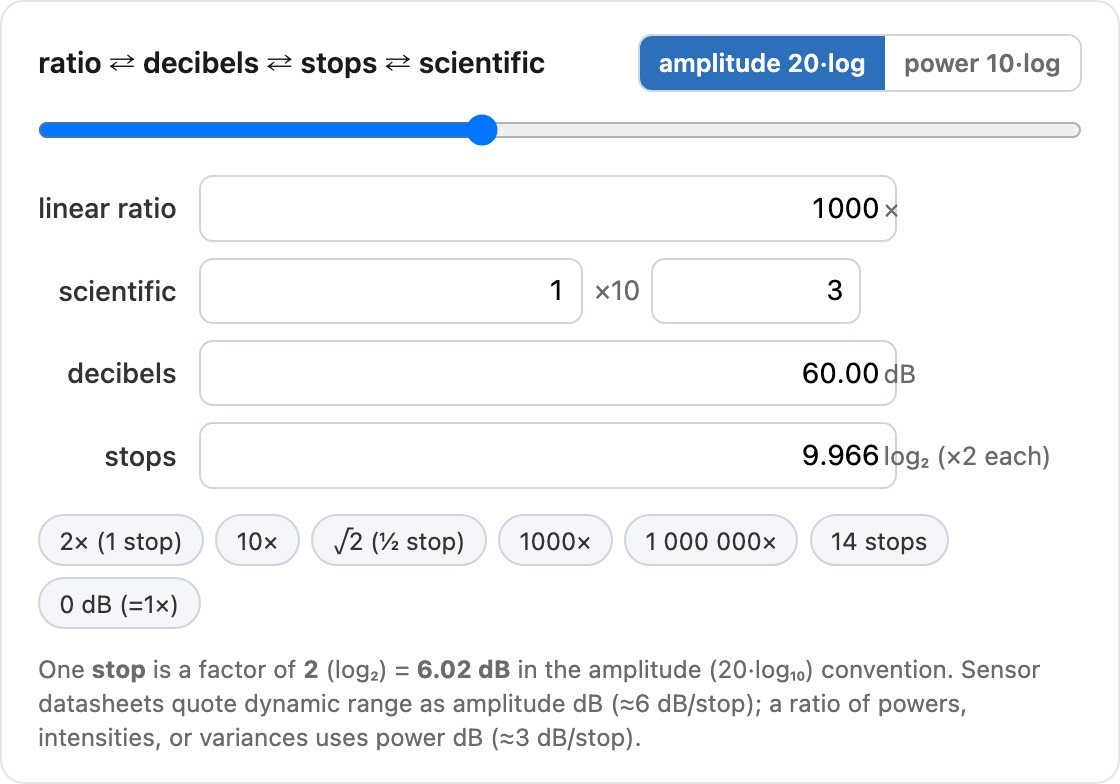
A word on the decibel itself, since it recurs through this chapter and the next. A decibel is just a logarithmic way to write a ratio: for a power (or energy, intensity, variance) ratio it is $10\log_{10}$, and for an amplitude (or voltage, signal) ratio it is $20\log_{10}$, the factor of two coming from power $\propto$ amplitude$^2$. Photographers count the same ratios in stops, factors of two ($\log_2$), so one stop is about 6 dB of amplitude or 3 dB of power. Decibels, stops, plain linear ratios, and scientific notation are thus four scales for the same underlying number, a multiplicative factor, and it helps to move fluently between them (Figure 2.8.5).
Shot noise is Poisson, so its variance grows linearly with the signal ($\sigma^2 \propto N$) and its standard deviation grows only as the square root ($\sigma \propto \sqrt{N}$). Two consequences pull in opposite directions: the absolute noise is larger in highlights than in shadows (a 10,000-photon highlight has $\sigma=100$; a 100-photon shadow has $\sigma=10$), yet the SNR $= N/\sqrt{N} = \sqrt{N}$ is higher in the highlights: the signal outgrows the noise. So bright areas are noisier in absolute terms but cleaner to the eye; the shadows have the worst SNR (Figure 2.8.4, Figure 2.8.6). This is why exposing to the right and brighter scenes look smoother, and why we gamma/log-encode so equal ratios get equal steps.
The affine model, whose full story is the next section, settles a lot of everyday "will this help my noise?" questions at a glance. Read each move against $\sigma^2 = g\,I + \sigma_r^2$ (signal $I$, photon-gain slope $g$, read-noise floor $\sigma_r$), tracking what happens to the signal, the noise $\sigma$, and their ratio. The entries below are for the shot-noise-dominated regime (well-lit midtones); the read-noise term $\sigma_r$ changes only the two rows that mention it.
| scenario | signal | noise $\sigma$ | SNR | what is really going on |
|---|---|---|---|---|
| raise ISO by 1 stop (×2 analog gain) | ×2 | ×2 | ≈ same | amplifies signal and noise together and adds no photons. Read noise, applied after the gain, shrinks relative to the signal, so deep shadows come out a touch cleaner. Not a substitute for light. |
| brighten by 1 EV in software (×2) | ×2 | ×2 | unchanged | multiplies values already recorded, so it amplifies the noise baked in at capture. No shadow benefit, unlike raising ISO at capture. |
| darken by 1 EV in software (×½) | ×½ | ×½ | unchanged | pure scaling; the ratio is untouched (though it can still clip or quantize). |
| average $N$ frames | ×1 | ÷$\sqrt N$ | ×$\sqrt N$ | independent noise partly cancels while the signal stays: the $1/\sqrt N$ law behind burst denoising and stacking. |
| sum $N$ values | ×$N$ | ×$\sqrt N$ | ×$\sqrt N$ | variances add, so SNR grows just like averaging; but read noise is paid $N$ times if the values are read separately. |
| charge-bin $N$ pixels (combine, then read once) | ×$N$ | ×$\sqrt N$ | ×$\sqrt N$, cleaner shadows | same shot noise as a digital sum, but read noise is paid once, not $N$ times. Check that the sensor actually combines charge before separate readout. |
| gather 2× the light (wider aperture or longer exposure) | ×2 | ×$\sqrt 2$ | ×$\sqrt 2$ | collects more photons per measurement, improving SNR before any reconstruction. Read noise unchanged. |
Software rescaling preserves SNR. Analog gain can reduce the relative contribution of noise added downstream, as the ISO section explains. Combining $N$ equally exposed independent measurements improves SNR as $\sqrt N$, while more photons per measurement improve the capture itself.
Image metrics⧉
PSNR⧉
optionalPeak signal-to-noise ratio expresses the same error in decibels:
Here $L$ is the fixed reference range: $1$ for normalized samples in $[0,1]$, or $255$ for 8-bit samples. It is not each image's measured maximum. For HDR values without a shared finite range, specify a normalization or use a measure designed for the intended luminance conditions. PSNR is not the sensor SNR discussed in Chapter 2.8, Noise, signal-to-noise ratio and dynamic range: the denominator here includes any discrepancy from the reference, including bias, blur, and registration errors.
Higher PSNR means lower MSE at the same $L$; zero error gives infinity. Halving MSE adds about 3 dB. There is no universal threshold for an acceptable image. Scores depend on the scene, encoding, crop, and degradation.
Be explicit about aggregation. Averaging image PSNRs differs from pooling squared errors and converting once, because the logarithm is nonlinear. For equal-sized images with MSEs $0.001$ and $0.01$ at $L=1$, the mean PSNR is 25 dB, while the PSNR of their mean MSE is about 22.60 dB. Report the convention and inspect the distribution, not only its mean.
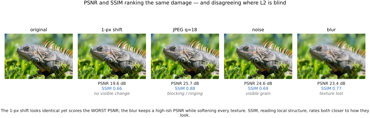
Linear RGB is useful for radiometric fidelity; a specified output encoding measures errors after rendering. Color differences such as $\Delta E$ in CIELAB address a different question, under a stated white point and viewing model; see Chapter 4.5, Advanced color: opponents, perceptually-uniform, and preferred. They do not account for spatial structure or automatically make an image-quality benchmark better. Do not apply an RGB PSNR peak to Lab channels and call the result comparable.
Bilateral filtering⧉
PS2 implements the bilateral filter (with a YUV chroma variant). → Chapter 1.5, Problem sets (appendix).
A blur mixes two sides of an edge and makes it soft. That is useful for some operations, but harmful when we want to remove noise while preserving sharpness or to smooth texture while keeping the boundary. The big idea of the bilateral filter is to only take into account pixels that are similar enough. This notion of affinity between pixels will come back over and over for edge-preserving techniques.
We illustrate bilateral filtering for the task of denoising, but it also underlies many algorithms because it enables the factoring of images into large-scale structure and local detail while preserving strong edges. This proves powerful for applications such as high-dynamic-range tone mapping (Chapter 18.3, Two-scale and bilateral tone mapping), upsampling low-resolution results, and combining images with different illumination, where the edges come from a second image (#Cross / joint bilateral).
Debugging: hand-checkable limits⧉
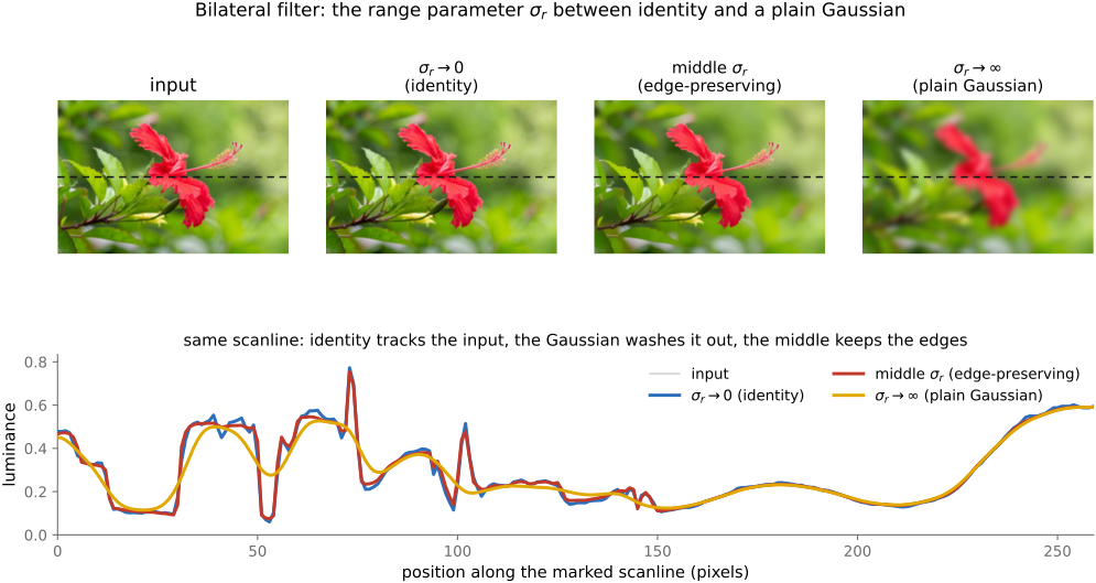
The bilateral has two limits you can predict by hand, and together they make an excellent correctness test for an implementation (Figure 10.1.7). Push the range width to each extreme:
- Large range variance ($\sigma_r \to \infty$): the range Gaussian flattens, $g_r \to 1$, so it does nothing: every value difference counts as "similar." The weight reduces to the spatial Gaussian alone, and the bilateral collapses to a plain Gaussian blur.
- Tiny range variance ($\sigma_r \to 0$): only neighbors with the same value retain weight in the limit. They may include many pixels, but averaging equal values leaves the output unchanged. Averaging those equal values changes nothing, and the output is the identity: the image comes back untouched, edges and all.
A middle $\sigma_r$ interpolates between these two: enough to smooth away noise and texture, not so much that it bleeds across real edges. If your implementation does not reproduce a Gaussian at large $\sigma_r$ and the identity at small $\sigma_r$, it is wrong. These are the first two things to check (and the recipe in the debugging sidebar above).
The same two knobs guide tuning. Pick $\sigma_s$ from the spatial scale of the structure you mean to remove (how large a region should be pooled). Pick $\sigma_r$ from the contrast of the edges you mean to preserve: set it just below the value jump of a real edge, so the filter smooths everything gentler than that and stops at anything sharper. And state the encoding first: the same numeric $\sigma_r$ means something completely different in linear light, in gamma, and in log luminance.
Bilateral filter⧉
Consider an input signal composed of a step edge with noise (Figure 10.1.1). The goal of bilateral filtering is to remove the noise by averaging nearby pixels without blurring the edge.
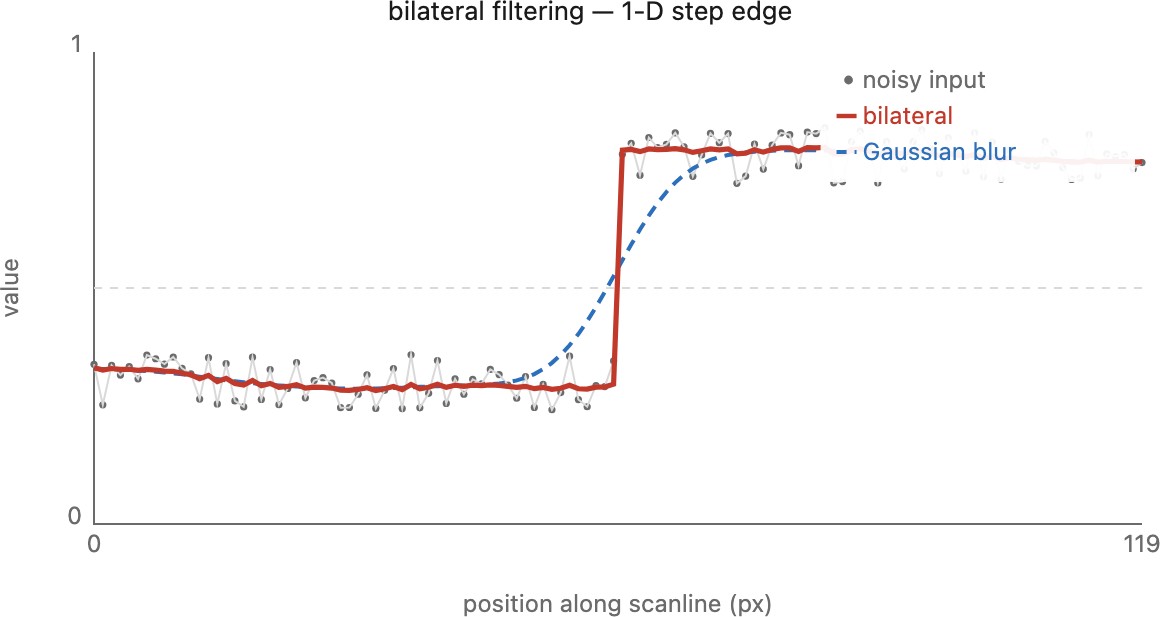
Start from the Gaussian blur. It replaces each pixel with a weighted average of its neighbors, where the weight only depends on distance. It is a spatial Gaussian $g_s(\lVert p - q\rVert)$ of the distance between the center pixel $p$ and a neighbor $q$: nearby pixels count for a lot, distant ones taper off. It is easiest to watch this on a 1-D scanline (a single row of the image), where the picture becomes a wiggly curve of value against position (Figure 10.1.1).
The trouble, once more, is the edge. A step edge on the scanline, with values low on the left and high on the right, gets smeared by the Gaussian, because right at the step the averaging window reaches across the boundary and blends the two plateaus together. The same bleed, in two dimensions and on a compressed base layer, is what paints halos along high-contrast edges in tone mapping (Chapter 18.3, Two-scale and bilateral tone mapping).
The fix is a single extra factor. Keep the spatial Gaussian, but multiply in a second Gaussian, this one on the value difference between the center pixel and the neighbor, $g_r(\lvert I_p - I_q\rvert)$. This range weight asks "are these two pixels similar in value?" and down-weights neighbors that are too different. A neighbor that is close in space but far in value, one on the other side of an edge, now earns a weight near zero, however spatially near it sits. The filter, all by itself, declines to average across the edge.
A practical wrinkle follows. The range weight asks whether two pixels are similar. But on a badly corrupted image the raw values are an unreliable judge: noise can make two same-region pixels look different, or two different ones look alike, so the weights themselves come out noisy. The weights need not be read from the original image at all. We can compute $g_r$ from a pre-cleaned version (a quick median filter, say, or any cheap denoise) and then apply those steadier weights when averaging the original pixels. Decoupling what decides the affinity from what actually gets averaged is exactly the move the cross / joint bilateral (below) makes with a separate guide image; using a median-filtered copy of the same image as that guide is just the in-place version of the trick.
Putting the two Gaussians together gives the bilateral filter (Tomasi & Manduchi 1998). The weight a neighbor $q$ receives at pixel $p$ is the product of the spatial and range terms,
and the output is the normalized weighted average of the neighbors,
In words: "average my neighbors, but only those that are both nearby and similar to me." The two widths do different jobs. $\sigma_s$, in pixels, sets how large a region we pool over, the reach of the spatial Gaussian. $\sigma_r$, in intensity units, sets what counts as "too different": the value gap beyond which a neighbor stops counting. Because $\sigma_r$ is measured in the same units as $I$, we must fix the encoding before we can quote it: for HDR tone mapping the filter runs on log luminance (Durand & Dorsey 2002, where a range $\sigma_r \approx 0.4$ in $\log_{10}$ is typical); other tasks may use linear values or a specified output encoding. There is no single required domain for every bilateral application.
As code, the brute-force bilateral is a double loop with a per-pixel normalization, and one subtlety distinguishes it from convolution: you may precompute the spatial weight $g_s$ (it is the same window everywhere), but the range weight $g_r$ must be recomputed for every pair, because it depends on the value difference at that pixel. The range function can be tabulated for quantized differences; it is the resulting image-dependent kernel that cannot be reused as one convolution. Specify spatial truncation and boundary handling, include the center sample, and accumulate in a sufficiently wide type.
precompute g_s over the window          # spatial weights, same for every pixel
for each output pixel p:
    sum ← 0;  W ← 0                      # accumulator and normalizer
    for each neighbour q in the window around p:
        w ← g_s(‖p − q‖) · g_r(|I[p] − I[q]|)   # range term recomputed per pair
        sum ← sum + w · I[q]
        W   ← W + w
    I_bf[p] ← sum / W                    # per-pixel normalization
For a color image the range distance $|I_p - I_q|$ is the 3-D distance in RGB (or YUV); everything else is unchanged.
The filter also travels under other names in editing software. Photoshop's Surface Blur is a bilateral filter: its radius is the spatial width and its threshold is the range width, over a box spatial kernel rather than a Gaussian. The name is worth knowing: those two sliders are the two widths of this section, and a tool many readers already use is a direct way to feel what each one does.
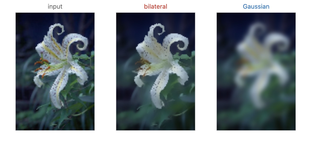
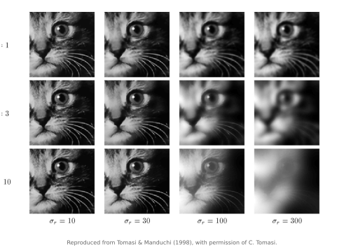
Two extreme settings of the range width $\sigma_r$ give two predictable outcomes that bracket the whole filter, the fastest way to sanity-check an implementation (the recipe also lives in Developing, testing & debugging). Figure 10.1.7
- Crank $\sigma_r$ very large. The range term flattens, $g_r \to 1$, and drops out of the product. The bilateral must collapse to a plain Gaussian, so run it side by side with your already-tested Gaussian blur; they should agree pixel for pixel.
- Shrink $\sigma_r$ very small. Now a pixel averages only with near-identical neighbors, so edges stay untouched and the output is essentially the input. Run it on a synthetic half-plane or rectangle (one hard edge): the bilateral must leave that edge razor-sharp.
If either limit misbehaves, the bug is in the range term or the normalization; fix that before trusting any middle $\sigma_r$.
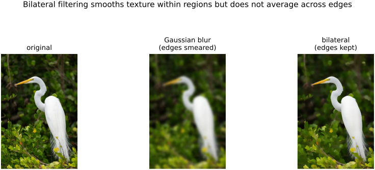
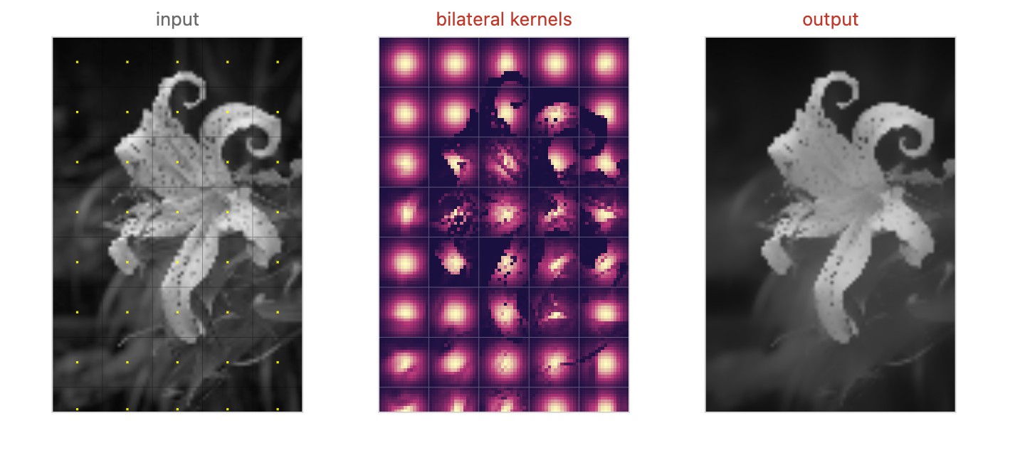
The 1-D picture carries straight to the 2-D image: the bilateral smooths flat texture and noise inside each region while holding the edges, so a portrait emerges with clean skin and intact eyelashes, and an HDR base layer stops cleanly at the silhouette instead of ramping across it (Figure 10.1.2).
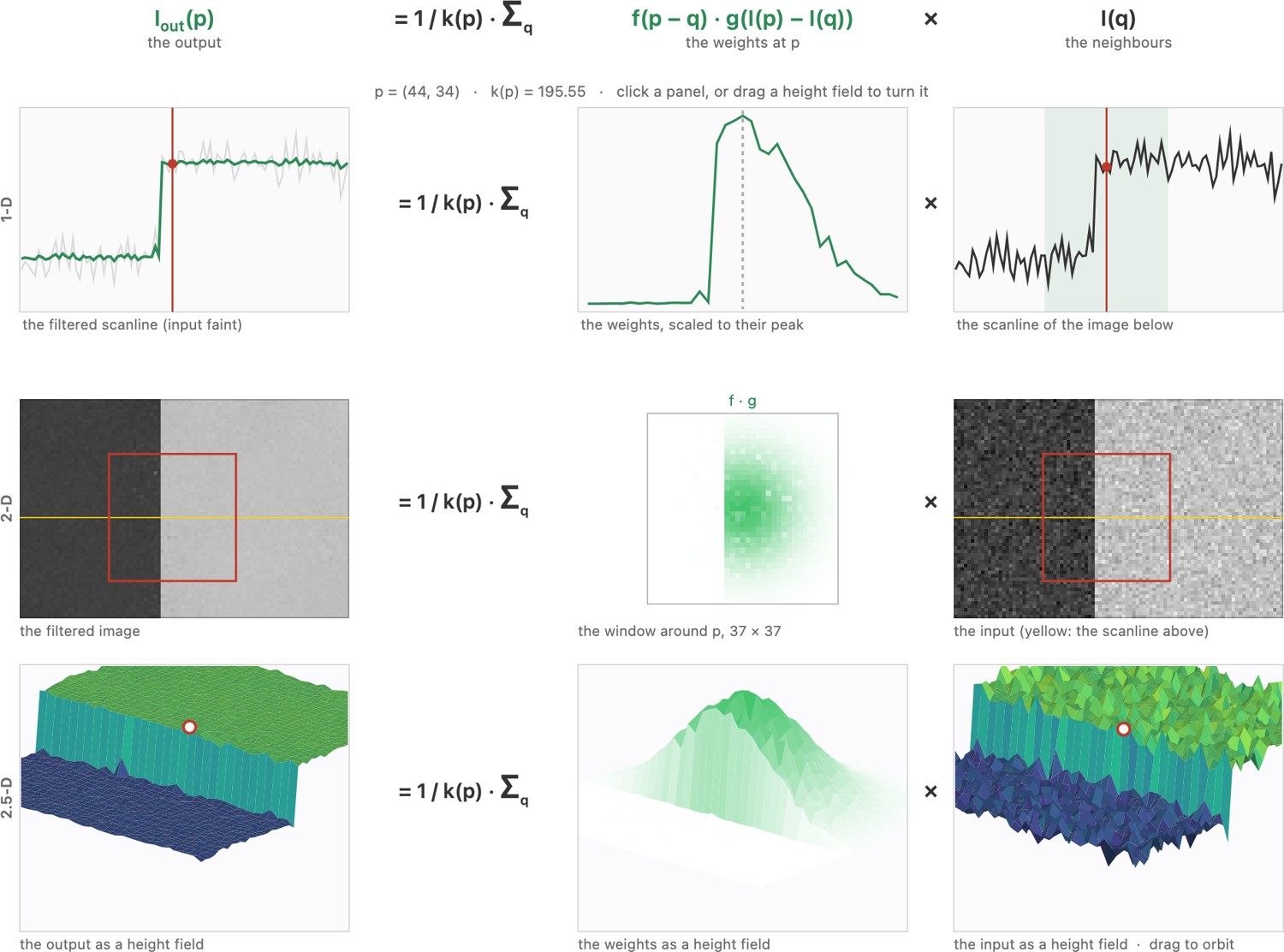
The range Gaussian $g_r$ is more than a clever weight; it is a similarity, an affinity between two pixels: a number that says how much these two pixels belong together, computed from their value difference. The bilateral averages pixels in proportion to that affinity. Every later method in this chapter, and several beyond it, is a different answer to one question: how should we measure whether two pixels belong together?
Use the color / intensity difference between two pixels as how much they belong together, an affinity, then average (or connect) pixels in proportion to it. Pixels with high affinity are treated as measurements of the same underlying thing and get averaged together; pixels with low affinity, across an edge, are kept apart. The bilateral filter's range weight $g_r$ is the first full instance, but the same affinity drives the bilateral grid, the guided filter, non-local means (NL-means), colorization, and matting / segmentation that follow. Edge-preserving is affinity. (This is L10.1, registered in Part 13, Denoising where the bilateral first appeared for noise; this is its full edge-preserving treatment.)
Robustness⧉
optionalWith the Gaussians defined above and the center included, $w(p,p)=1$, so $W_p\geq1$. The normalized bilateral is a convex average and cannot blow up from division by a near-zero normalizer. An isolated value can still be poorly denoised because it assigns little weight to other samples. This is a limitation of the affinity, not proof that normalization is numerically invalid.
The deeper weakness is that the range term reads the noisy image itself. At an outlier the center's own corrupted value decides which neighbors count as similar, so the pixel that most needs help is the one whose weights are least trustworthy: it finds nothing that resembles it and averages with almost nothing but itself. A hot pixel survives the filter for the same reason an edge does.
A cheap repair is to compute the range term from a pre-filtered copy instead of from the input. Run a small median filter first, then use that image as the reference for the value differences while still averaging the original samples. The median removes impulses without moving an edge (Chapter 13.3, Gaussian, median, and bilateral filtering), so the weights are decided by something close to the clean signal while the output remains an average of real measurements. Mechanically this is the cross-bilateral construction of the next section, with the guide derived from the input rather than captured separately.
The cost is that the guide's failures become the filter's. A median erases thin lines, small dots and isolated highlights, and a structure the guide has removed has no range weight left to defend it: the bilateral will happily average it away. Check the guide on the structures you care about before trusting the result, and keep the median's window small enough that it removes impulses rather than detail.
An alternative discussed by Aubry et al. is an unnormalized correction Aubry et al. 2014. Its scale must be defined. With these unnormalized spatial weights, introduce a step size $\eta$:
Each neighbor contributes a weighted difference from the center. A sufficient condition for this update to remain a convex combination is $0\leq\eta\sum_{q\ne p}w(p,q)\leq1$. One practical convention normalizes the spatial kernel to sum to one and uses $0\leq\eta\leq1$. Without a scale convention, adding more neighbors can cause overshoot. The update generally differs from the normalized bilateral; neither is a universal replacement for the other.
This unnormalized form is also the bilateral cousin of the local Laplacian filters: working in deltas from the input, scale by scale, is exactly the move that makes the multiscale local Laplacian fast and robust (Paris / Aubry; cross-ref Chapter 10.4, Local Laplacian filters and Chapter 6.6, Pyramids and wavelets).
Removing the bilateral normalizer changes the filter. Specify a normalized spatial kernel or an explicit step size, then test constants, impulses and edges. A small total affinity makes a small correction; it does not establish that an isolated value is correct.
Cross / joint bilateral⧉
optionalSo far the affinity has been read off the same image we are smoothing (the range weight uses $I$ itself). But there is no reason it must. The cross (or joint) bilateral filter reads the range weight from a different image, a guide $J$, while still averaging the target $I$:
The averaging runs over the target $I$; the affinity comes from the guide $J$. Why want that? Because sometimes the image you wish to smooth is too noisy or too dark for its own edges to be trusted. If you read the affinity off $I$, you are reading off the noise. If you hold a cleaner signal that shares the same scene geometry, borrow its edges instead.
The headline application is flash / no-flash photography (Petschnigg et al. 2004; Eisemann & Durand 2004). Shoot a dim scene twice: once without flash (the right mood and color, but dark and noisy) and once with flash (clean and well-exposed, but flat, harsh lighting). After registration, many object boundaries correspond. Motion, occlusion, flash shadows and specularities can introduce mismatched edges, so a practical pipeline needs confidence masks or fallback behavior. So smooth the noisy no-flash image using the flash image as the guide: the flash image's clean edges drive the range weight, telling the filter where it may and may not average, while the values being averaged come from the ambient no-flash shot. The result keeps the no-flash mood and kills the no-flash noise (Figure 10.1.8). We develop the full flash/no-flash pipeline later (forward-ref → Flash / no flash, computational illumination).
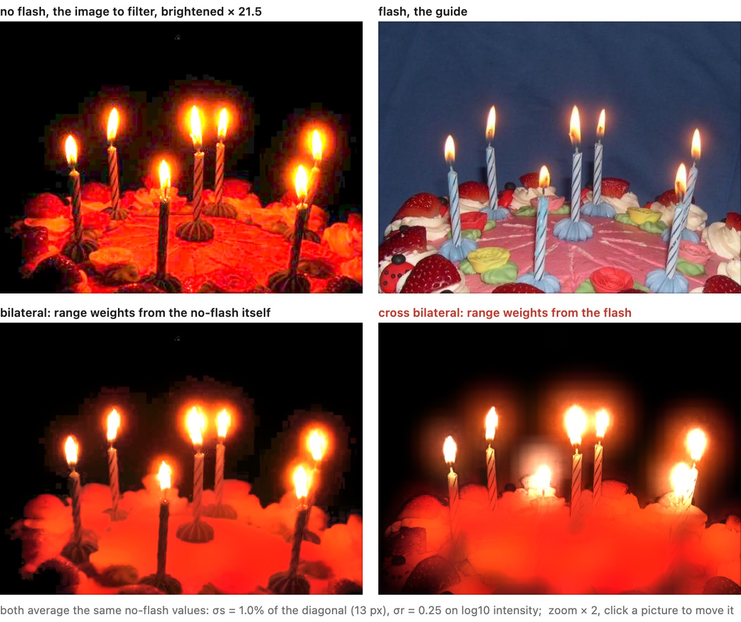
The full flash/no-flash story, including Petschnigg's detail transfer, Eisemann & Durand's intrinsic-relighting pipeline, flash-shadow removal, and their end-to-end results, belongs with the rest of computational illumination, where capturing the scene under two lights is the whole subject (Flash / no flash).
The cross bilateral is the first instance of a more general joint / guided idea (filter one image using structure taken from another) that culminates in the guided filter (later in the part).
Brute force⧉
Brute-force translational alignment (SSD / NCC)⧉
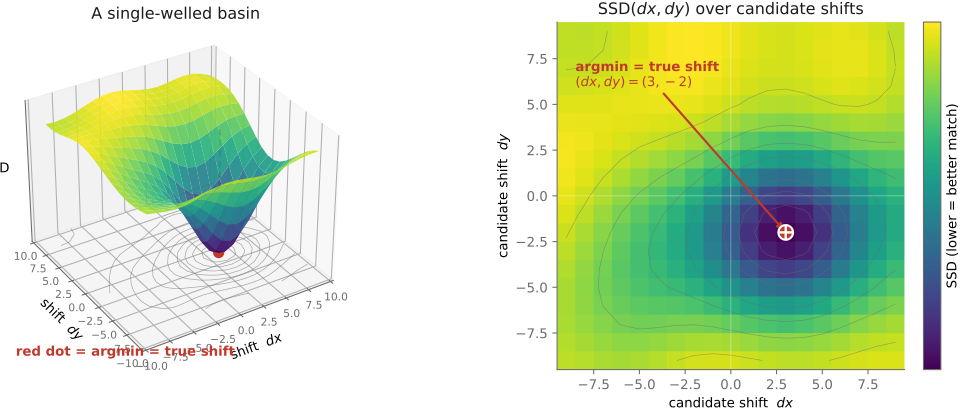
For a tight burst the whole image slides as one rigid 2-D shift $(dx,dy)$, and the simplest aligner imaginable just tries every shift in a search window and keeps the best-scoring one. A double loop over $(dx,dy)$, with no cleverness at all, is useful here because it leaves little room for implementation errors. Everything then rides on the score: the function that says how well two frames agree at a given candidate shift (Figure 12.1.2).
The default score is the sum of squared differences (SSD),
SSD is small when the sampled intensities agree, which need not happen at a unique displacement. Repeated patterns create several minima; flat regions create weak curvature. Same exposure does not guarantee brightness constancy, and an HDR bracket can add clipping and motion. Mean-subtracted normalized cross-correlation handles a positive affine intensity change on the evaluated region:
NCC subtracts the mean and divides by the norms of the centered patches. It is invariant to positive gain and constant offset when neither patch is constant. Mask clipping and invalid pixels; do not divide by nearly zero variance. Nonlinear tone changes and spatially varying illumination require a better model than a single gain and offset.
Two practical notes. First, the cheapest unit test you will ever write: align a synthetic image to a known shift of itself and confirm the minimum lands exactly there, by construction. Catch the indexing, sign, and interpolation bugs on that toy, not on noisy real frames where a one-pixel error hides in the grain. Second, sub-pixel accuracy: the integer-grid minimum is rarely the true minimum, so fit a parabola to the SSD basin (or upsample the surface) and read off the vertex to get a fractional shift, realized by bilinear or bicubic interpolation when you resample. Those tiny fractional offsets are noise to be removed when you are denoising, but they are signal to be exploited when you are super-resolving: a burst whose frames are sub-pixel-shifted samples the scene more densely than any one frame can, which is precisely what burst super-resolution mines (Wronski et al. 2019 Wronski et al. 2019; cross-ref Chapter 14.2, Multi-frame super-resolution).
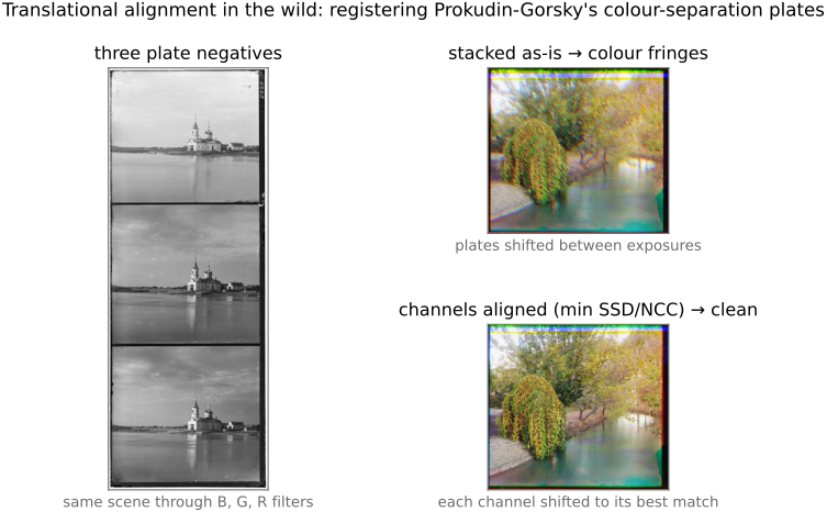
Prokudin-Gorsky’s sequential color-separation captures provide an early alignment example Prokudin-Gorskii. NCC can be a useful baseline for their digitized channels, but spectral color differences are not generally a single gain and offset. Gradients, suitable crops and rejection of damaged or moving regions may improve the estimate (Figure 12.1.4).
Both steps can be run on a real burst: search the window, read off the shifts, and average with and without them (Figure 12.1.3).
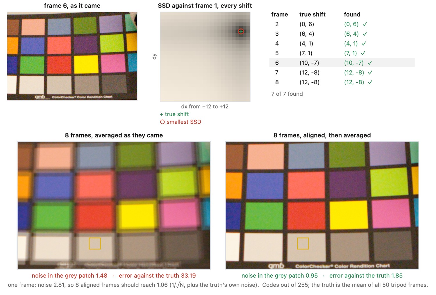
Compare candidate shifts over a common valid support, or normalize a masked score by a sufficient valid-sample count. Otherwise larger shifts can win merely by discarding difficult pixels. A low residual and a high margin over competing shifts are complementary checks; neither detects all model mismatch.
The separated color exposures of Prokudin-Gorsky provide a useful application Prokudin-Gorskii. Shifted channels turn an otherwise sharp edge into red and cyan fringes when the plates are stacked. Search for a translation of each channel relative to a reference and inspect whether those fringes shrink. However, a red object can be bright in one filtered exposure and dark in another. Normalized correlation compensates for a common offset and scale, not for every spectral difference between objects. Comparing gradients or selecting regions with shared structure can help. Motion between exposures remains a separate problem that a single channel translation cannot fix.
Coarse-to-fine alignment on a pyramid⧉
optionalBrute force has two failure modes that bite together. Large motion forces a large, and therefore expensive, search window; and a raw SSD surface is not always the clean single-welled basin of the idealized figure. Repetitive texture (a brick wall, a picket fence) and aliasing carve local minima into it, and a local refinement started far from the answer can fall into the wrong well. An exhaustive search finds the best score in its window, though that score may favor a false match. Going multiscale addresses both, though only the first reliably (Figure 12.1.6).
Build a Gaussian pyramid of both frames and align coarse-to-fine (the pyramid of Chapter 6.6, Pyramids and wavelets, here repurposed as a search strategy). At the tiny, heavily-blurred top of the pyramid, a small search in pixels covers a large real motion, because each coarse pixel stands for many fine ones, so large displacements become cheap. Better still, the low-frequency surface at the top may be smoother because blurring attenuates high-frequency detail, often making a rough estimate easier to obtain. Propagate that estimate down to the next level, scale it up, and refine it with a tiny local search; the high frequencies you add as you descend mostly refine the estimate, because the local search at each level is too small to jump to a distant minimum. That is also the risk: if the coarse estimate is wrong, the finer levels rarely recover.
Pyramids can smooth the cost and reduce a large displacement to a smaller coarse-grid shift. They do not guarantee one clean basin: periodic texture and lost small structures can remain ambiguous. Verify the refined result on the original images.
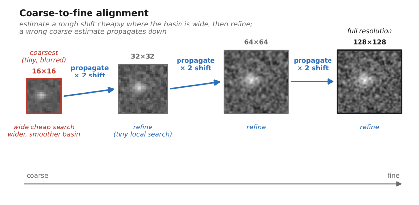
Build each level by filtering before decimation. Otherwise the coarse image can contain alias patterns that disagree between frames, creating false evidence for motion. A pyramid is useful both as a representation and as a search strategy: solve large motions on a coarse grid, then recover precision from finer samples. HDR+ applies this idea to tiles before robust burst merging Hasinoff et al. 2016. Local refinement should still be checked against alternatives when the coarse choice is ambiguous.
Denoising by averaging⧉
Photograph a gray card several times without changing the camera settings. The value at one pixel fluctuates, but the average becomes more stable as the number of frames grows. Chapter 2.8, Noise, signal-to-noise ratio and dynamic range established the $1/\sqrt N$ law. Here we derive it for a frame stack and examine what happens when motion, outliers, or calibration errors violate its assumptions.
Fix the exposure, gain, and processing; keep the illumination stable; and align corresponding scene points before combining their measurements. Use linear values with the black level removed and preserve negative noise excursions. Under these conditions, independent zero-mean errors average out. They need not be Gaussian or symmetric: an unclipped Poisson count is unbiased even at low light.
Recording several captures lets us choose or combine their measurements afterward. A filter wheel is the plain example: shoot the scene through a red, a green and a blue filter (or through a polarizer at several angles) and the choice of how to combine the bands can be made later, at the desk. Exposure brackets, focal stacks, and panoramas extend this idea to different capture settings.
Several compatible measurements can reduce uncertainty or cover information missing from one frame. This is a different benefit from the previous lesson. Deferring a choice picks among things one exposure could have recorded; combining exposures can exceed what any single exposure could record, such as a noise level below one frame's, a dynamic range wider than the sensor's, or a depth of field deeper than the aperture allows. The reconstruction must account for differences in exposure, focus, viewpoint, or scene motion.
Why averaging works: the $1/\sqrt N$ derivation⧉
Let $X_i=\mu+n_i$ be the measurement of one scene point in frame $i$. The desired signal is $\mu$, and the errors satisfy $\mathbb E[n_i]=0$, $\operatorname{Var}(n_i)=\sigma^2$, and independence across frames. Equal variance is a per-pixel assumption across the stack; it does not require bright and dark pixels to have equal noise.
The estimate is $\bar X=N^{-1}\sum_{i=1}^{N}X_i$:
mean = zero_image()
for frame in aligned_linear_frames:
    mean += frame
mean /= number_of_frames
Its expected value is
Thus the estimator is unbiased: over repeated stacks, its average equals the true signal. An individual finite stack still contains error. Scaling a random variable by $1/N$ scales its variance by $1/N^2$, and independent variances add, giving
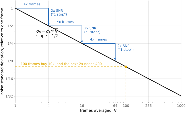
Nothing is blurred by this, which is what separates it from every single-image method in the part: each pixel is averaged only with repeated measurements of itself, never with a different pixel. The cost is in the exponent. Halving the noise again takes four times as many frames, so there are sharp diminishing returns to spending photons this way (Figure 13.2.1).
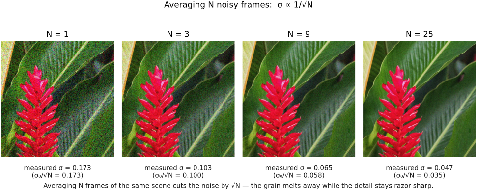
The signal stays constant while the noise standard deviation falls. Figure 13.2.2 shows the resulting narrowing of a flat patch's histogram.
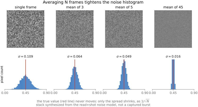
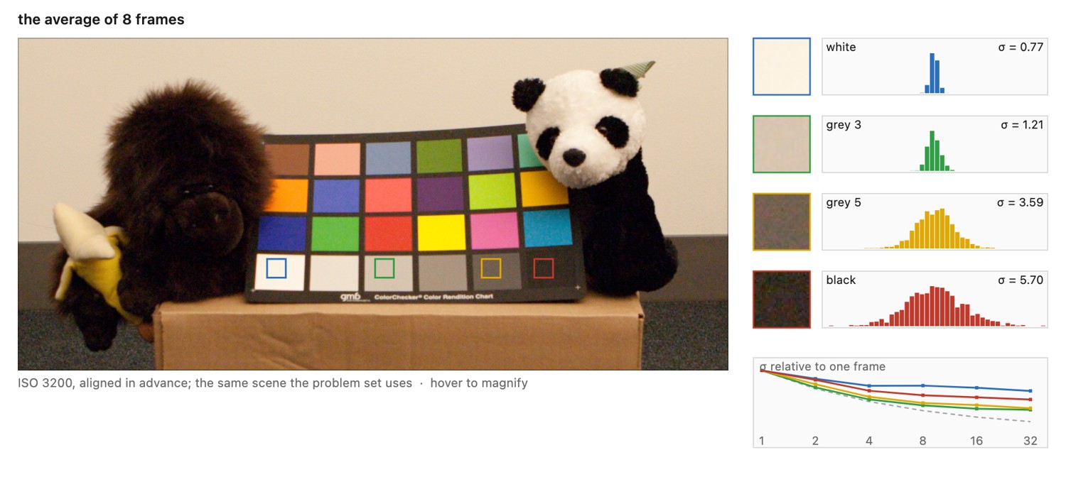
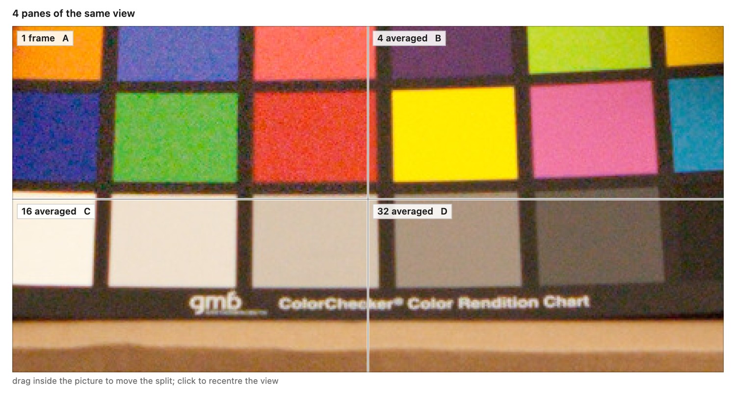
Averaging four independent measurements of the same signal halves the noise standard deviation. Averaging 100 reduces it by a factor of ten. These statements require zero-mean errors and unchanged per-frame variance. Lowering the effective noise floor can extend the usable range, as described in L2.46, provided the captures have not clipped the signal.
SNR increases by $\sqrt N$, or $10\log_{10}N$ dB: about 3 dB per doubling of the frame count (Figure 13.2.5). This comparison adds capture time while holding each exposure fixed. It does not say that splitting one fixed total exposure into more frames improves SNR.
The same stack estimates the per-frame variance:
The divisor $N-1$ corrects for estimating the mean from the samples whose deviations we measure. For two fair coin flips coded as 0 and 1, the four outcomes give sums of squared deviations $0,\tfrac12,\tfrac12,0$. Dividing by two gives an average estimate of $1/8$, half the true variance $1/4$; dividing by one gives $1/4$.
If errors are correlated, the omitted terms return:
A common offset across frames does not diminish. A fixed calibration bias survives as an error in the mean even when the remaining random fluctuations obey the averaging law.
A four-frame example separates the two assumptions. If the same signal is measured four times with independent errors of standard deviation 8, their average has standard deviation 4. A fixed offset of 3 at that sensor position survives unchanged: averaging adds the offset four times and divides by four. A fluctuation shared by every frame likewise does not receive the independent-noise reduction. Thus a cleaner-looking average can still retain a structured bias. Calibration and averaging solve different parts of the measurement problem, as developed in Chapter 2.8, Noise, signal-to-noise ratio and dynamic range.
The square root also describes the diminishing return on capture time. Halving the noise standard deviation takes four times as many independent, equally exposed frames. Going from one frame to four and from four frames to sixteen buys the same factor of two, but the second improvement costs twelve extra frames. Motion, storage, and latency can make those extra frames more expensive than the noise reduction is worth.
When the plain mean is wrong: robust combination⧉
optionalA satellite crossing one exposure adds a bright streak to the stack. The mean reduces its contribution by $N$, but leaves a visible trace. A per-pixel median is less sensitive to a small number of extreme values (Figure 13.2.6). It can still fail when the wrong scene or moving object supplies most of the samples at that position.
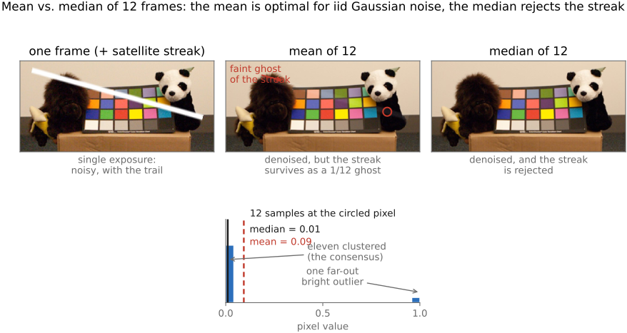
For independent Gaussian samples of a constant signal, the large-sample variance of the median is approximately $\pi/2$ times that of the mean. Its standard deviation is about 1.253 times larger, corresponding to roughly 20% lower SNR. Robust rejection therefore has a cost when all samples follow the assumed Gaussian model.
Sigma-clipping rejects measurements whose deviations exceed a chosen multiple $k$ of an estimated standard deviation. A robust initial center and scale prevent one large outlier from inflating its own rejection threshold. The following is an illustrative procedure for a sufficiently large stack, not a guarantee for a short burst:
for each output pixel p:
    values = valid_registered_samples(p)
    if values is empty:
        mark_output_invalid(p)
        continue
    center = median(values)
    scale = max(1.4826 * median(abs(values - center)), noise_floor(p))
    keep = abs(values - center) <= k * scale
    if too_few_samples(keep):
        out[p] = center
    else:
        out[p] = mean(values[keep])
The factor 1.4826 calibrates the median absolute deviation for Gaussian noise. Choose $k$ and the minimum sample count using the noise model; rejection based on a short stack can discard valid measurements or retain an outlier. Winsorization, which caps extreme values, is distinct from discarding them. Moving boundaries and occlusion usually need alignment confidence and region-dependent weights in addition to a per-pixel test.
For independent unbiased measurements of unequal known variances $v_i$, the minimum-variance linear unbiased estimate uses
Before combining different exposures, convert them to a common signal scale and transform their variances by the square of the same scale factor. Derive weights from calibrated parameters or a stable estimate, since weighting directly by a noisy measured value can bias the result. Noise-optimal HDR capture uses this relationship to select exposures and combine their useful ranges (Hasinoff et al. 2010).
This is the same neighborhood-selection question that appears in edge-aware filtering, now asked across frames. A sample can be nearby after alignment yet belong to a different surface because of motion or occlusion. Rejecting it prevents a ghost, but reduces the amount of independent evidence available there. HDR merging faces the same compromise, with the additional need to reject saturated measurements.
Handheld low light: the phone in your pocket⧉
optionalA handheld burst replaces one motion-blurred long exposure by several shorter measurements. The merge aligns stable regions and reduces the contribution of measurements that disagree because of motion or occlusion. Near a moving subject, fewer usable samples mean less noise reduction. A single frame count therefore does not describe the quality everywhere in the result.
HDR+ combines burst capture with alignment and noise-aware merging (Hasinoff et al. 2016). Night Sight also estimates motion to choose exposure durations and frame counts, and uses low-light white balance and tone rendering (Liba et al. 2019). These later operations affect the appearance, so a clean-looking output should not be attributed to averaging alone. Chapter 23.3, Focal stacks and depth of field extension considers related capture-time tradeoffs involving aperture and focus (Hasinoff & Kutulakos 2009).
Night Sight makes the capture decision part of denoising Liba et al. 2019. A relatively still scene permits longer individual exposures, reducing how often read noise is incurred for a given light budget. Subject motion favors shorter exposures, which reduce blur within each frame but make each measurement noisier. Motion estimation therefore helps choose exposure durations and frame counts before the burst is combined. Alignment and robust merging then handle disagreement among frames. Low-light white balance and tone rendering address different questions afterward: a low-noise estimate can still have an unwanted cast or look unlike a night scene. The complete result depends on capture, combination, and rendering together.
Recovering a clean signal does not determine how bright a night photograph should look. A sufficiently long exposure can make a moonlit landscape resemble daylight. The Night Sight team drew on illusionistic painting to preserve the impression of night: strong contrast, dark surroundings, and shadows that approach black, even while revealing more color and detail than the eye could see. Their tone curve balances visibility against that impression of darkness. This is a rendering decision after reconstruction, and a useful connection to the discussion of pictorial cues and adaptation in the color and perception parts (Google's account of Night Sight).
Gaussian, median, and bilateral filtering⧉
A noisy photograph of a wall contains nearby pixels with similar clean values. Averaging them reduces noise. At the wall's boundary, however, the same operation mixes two surfaces and blurs the edge. Single-image local denoising must decide which neighbors can supply useful evidence about a pixel.
Everything in this chapter is a different answer to one question: which neighbors count as measurements of the same value? In a flat region every neighbor qualifies and averaging cleans up beautifully. At the boundary between a dark cake and a bright wall the neighbors on the far side are measurements of something else, and averaging them smears the two into a muddy band.
We compare a fixed Gaussian average, a median, and a bilateral average whose weights depend on the measured values. Their assumptions differ, and none guarantees preservation of every small feature. The derivation below uses independent zero-mean noise of constant variance in one channel; raw signal-dependent noise requires calibrated local variances or stabilization (Chapter 13.1, Noise models, transforms, and benchmarks).
Gaussian smoothing, and the assumption inside it⧉
Averaging a neighborhood assumes that every pixel in it is a measurement of the same underlying value, corrupted independently (the image is locally constant). Where that holds, the average is the right estimate and the noise cancels out. Where it fails, in particular at any boundary between two surfaces, the average mixes two different values and returns something that was never in the scene. A Gaussian kernel softens the assumption by trusting near neighbors more than far ones, but it still applies the same fixed weights at every pixel, whatever the image is doing there.
For analysis, consider a fixed clean image $x$. What varies is the measurement: the measured value is the truth plus an error, $y_q = x_q + n_q$, and the error is a fresh draw every time the shutter opens (Chapter 13.1, Noise models, transforms, and benchmarks).
For now, we assume two important properties of those draws. First, they average out, meaning the error at a pixel tends to zero as the number of shots increases. Second, they are independent between pixels: knowing that a photosite read high says nothing about its neighbor. That is true of shot noise and read noise, and false of fixed-pattern response and of noise that has already been through demosaicking or resampling. The variance $\sigma^2$ is the size of a typical error, squared; a refresher on these terms is in Refreshers#Probability and information theory.
Because noise is probabilistic, we analyze denoising through the thought experiment of shooting the same scene a large number of times with different noise instances each time. We then conceptually run the same filter on each frame and look at one output pixel across all the different results. We then characterize the performance of the method via statistical estimates such as the average squared error. This is related to the denoising by averaging technique studied in Chapter 13.2, Denoising by averaging but here the goal is to understand the expected error in one run via a probabilistic average error analysis, not to actually compute averages to reach the value of a pixel.
The average error can manifest in two main ways. The answers can be scattered, which means the filter still passes noise through. And their center can sit away from the truth, which means the filter has mixed in something that was never at this pixel. The first is the variance of the estimate, the second is its bias, and the error that matters, squared and averaged, is the bias squared plus the variance. A denoiser is an attempt to make that sum small.
A normalized Gaussian kernel supplies fixed nonnegative weights $w_{pq}$ that decrease with distance from the output pixel $p$:
For independent errors of equal variance $\sigma^2$, the output variance and bias are
The bias formula is important because it is the only place the noise-free image itself appears. The term $x_q-x_p$ captures the deviation from the assumption of a locally constant image. Let's look at variance and bias on two patches. On a flat patch every $x_q$ equals $x_p$, so every term of the bias is zero, and with a box of nine equal weights the variance is $\sigma^2/9$: the noise standard deviation falls by three, and nothing is lost. Now slide that same window onto an edge where the far side is 100 units brighter, with half the weight landing across it. The variance is unchanged, still $\sigma^2/9$, while the bias is about 50 units, next to a noise level of perhaps two or three. The filter has not failed at its job; it has done exactly what it was told, on an assumption that stopped being true.
This is called the bias-variance tradeoff. Widening the kernel moves both terms at once, buying variance with bias, and no choice of width escapes the trade: at any setting, a fixed kernel that is wide enough to clean the flat regions is wide enough to damage the edges. That is why the chapters after this one change the weights rather than the width, why Chapter 13.12, Measuring a denoiser compares two denoisers at a matched operating point rather than at matched parameters, and what Chapter 13.13, The limits of denoising pushes to its bound.
Define the effective sample count $N_{\mathrm{eff}}=1/\sum_qw_{pq}^2$, which is the number of independent samples the weighted average is worth. Equal weights over $N$ independent samples give $N_{\mathrm{eff}}=N$ and recover the averaging law of Chapter 13.2, Denoising by averaging; a Gaussian gives rather fewer than its tap count, since the outer taps contribute little.
Choosing the width is therefore choosing what to sacrifice. Set $\sigma_s$ from the size of the structure you are willing to lose: everything substantially smaller than the kernel is on its way out, and everything substantially larger survives with its edges softened. In practice the Gaussian is also the cheap choice, because it is separable and a two-dimensional blur costs two one-dimensional passes (Chapter 6.2, Convolution).
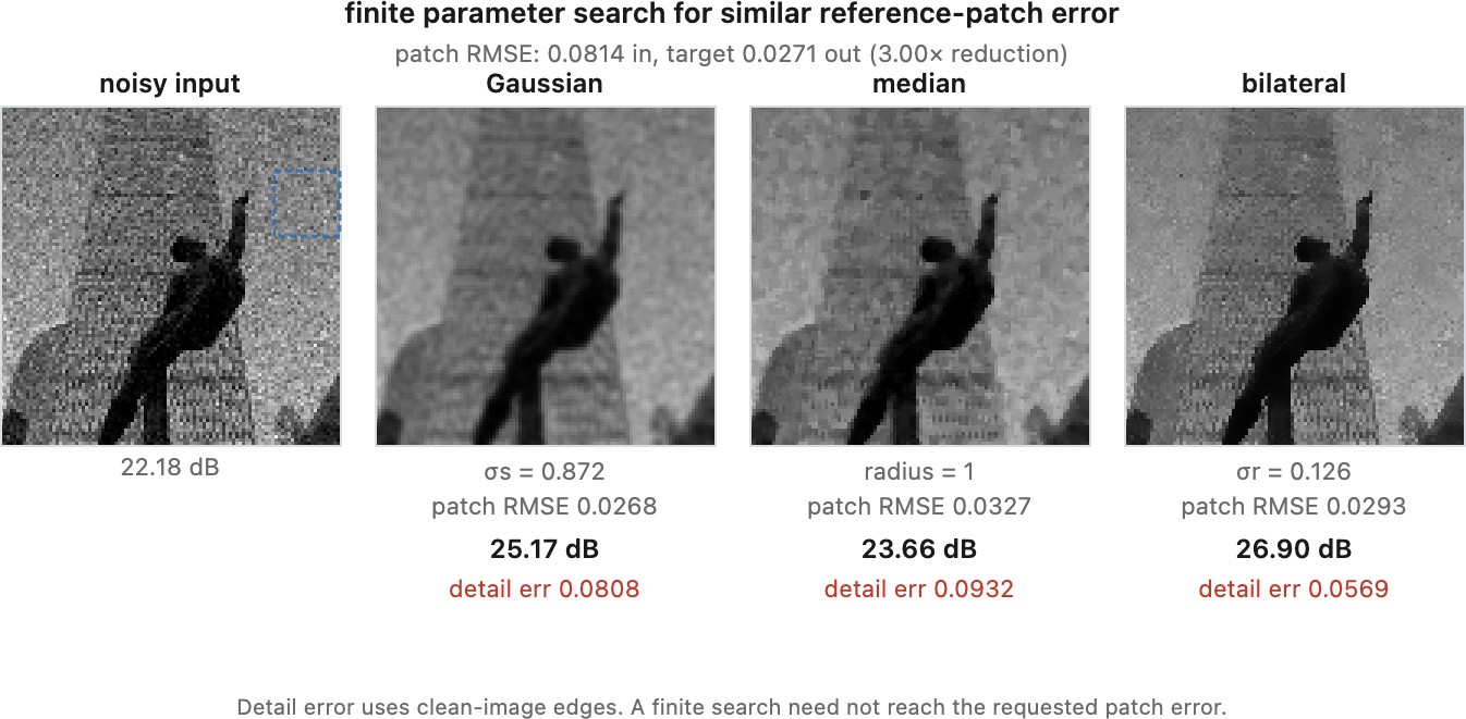
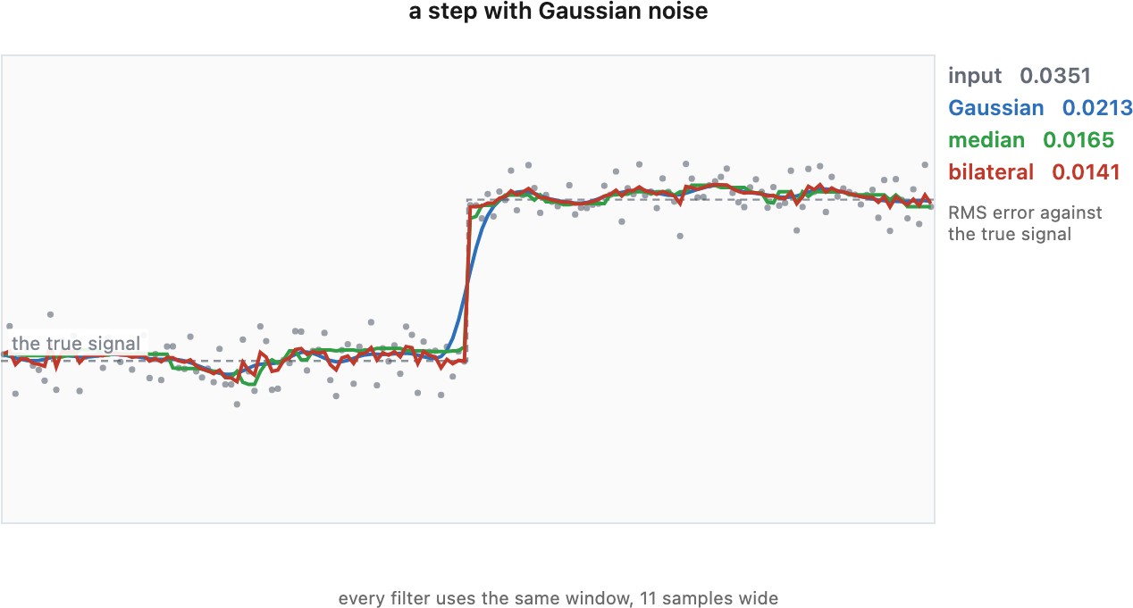
Start with the Gaussian alone in that panel, and set the other two aside until the sections that introduce them. Widen it and watch the two terms trade: the flat patch cleans up, the edge softens, and the residual view fills with the structure the filter took.
The frequency picture says the same thing and explains why blurring is worth doing at all. White noise has a flat power spectrum, so it carries as much energy at high frequencies as at low. Photographs do not: most of their energy sits at low frequencies, and the fine detail that occupies the high end is a small part of the total. A low-pass filter therefore discards a large share of the noise and a small share of the signal. That argument has an optimum, and the optimum is not a Gaussian.
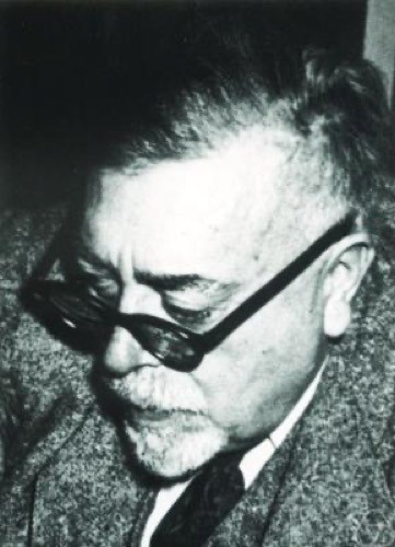 For a stationary signal and independent additive stationary noise with known power spectra, the minimum-MSE convolution has frequency response $H=S_x/(S_x+S_n)$. It attenuates frequencies dominated by noise. Its optimality is conditional on those spectra and the linear, shift-invariant class; natural images have spatially varying structure. Norbert Wiener (1894–1964), MIT mathematician and founder of cybernetics, derived this optimal filter from his World War II work on anti-aircraft fire control. Portrait: Konrad Jacobs, Oberwolfach, CC BY-SA 2.0 DE, via Wikimedia Commons.
The Wiener filter Wiener 1949 is what the frequency argument looks like when it is pushed to its conclusion: keep each frequency in proportion to how much of it is signal rather than noise. Its assumptions are the catch. It needs both spectra in advance, and it treats the image as one stationary process, when a photograph is a collection of regions with different statistics. A filter that could vary its behavior by region would do better, which is the move the rest of the chapter makes.
The two expressions above are exact for fixed weights and independent errors. Three departures matter in practice.
- Unequal variances. With independent but differing $\sigma_q$, the output variance is $\sum_qw_{pq}^2\sigma_q^2$. In raw, where the variance rides the signal, a neighborhood spanning bright and dark is a weighted average of unequal-quality measurements.
- Correlated errors. Any correlation needs the covariance terms, and demosaicking, resampling and lens shading all introduce it. Noise that has been through a pipeline is not the noise the formula assumes (Chapter 13.1, Noise models, transforms, and benchmarks).
- Repeated taps at a boundary. With a replicated border extension, several kernel taps can address the same sensor sample. Combine their weights before squaring them: repeated reads of one sample are perfectly correlated, not independent evidence. Counting taps instead overstates $N_{\mathrm{eff}}$ exactly where the estimate is already weakest.
None of this applies cleanly to weights computed from the noisy image itself, which is what the bilateral filter does later in this chapter.
The median, and the noise it is actually for⧉
optionalThe median selects the middle value of a sorted neighborhood. It is also a minimizer of
Changing an outlier's magnitude can move the mean arbitrarily far, but need not move the median. For example, the values $10,10,11,11,255$ have mean 59.4 and median 11. This makes the median useful for sparse impulse corruption (Figure 13.3.3).
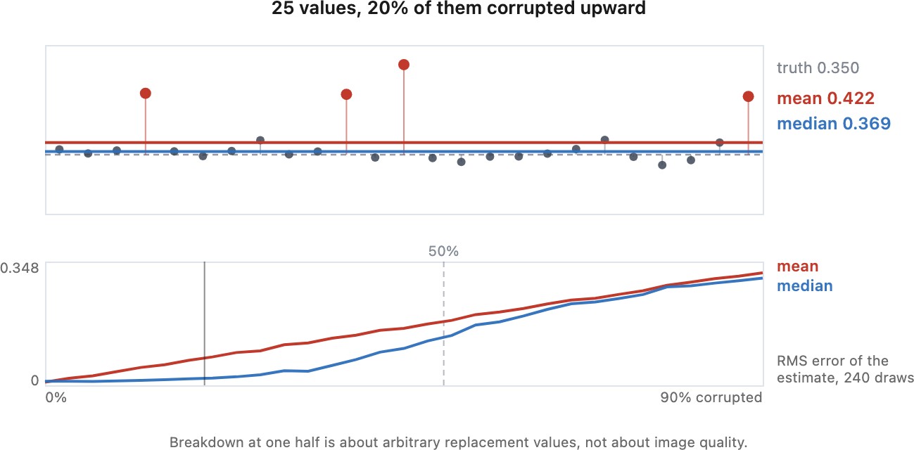
For a constant signal with independent Gaussian errors, the sample median's large-sample standard deviation is about $\sqrt{\pi/2}=1.253$ times the mean's. Robustness is useful when outliers are present, but has an efficiency cost when they are absent.
A median can preserve an ideal step when the correct side supplies a majority of the window. The same majority rule removes thin lines, isolated stars, and small details, and can round corners. It is nonlinear, so it has no single convolution kernel or frequency response. Repeated passes are not equivalent to one pass with a larger window. Iterating one median does, however, stop changing things: for a finite 1-D signal, repeated passes converge to a root signal that the filter leaves unchanged, made of constant runs and monotone stretches long enough to survive the window Gallagher & Wise 1981. Further passes then do nothing.
The median's majority rule explains both a strength and a failure. In a window containing mostly dark background and one extreme bright outlier, the middle sorted value remains dark. That suppresses a hot pixel, but it can also suppress a real isolated star or a thin bright line. At a broad ideal step, the side occupying most of the window determines the answer. The filter has no knowledge of which small structure the photographer intended to preserve. Inspect small real details as well as the removed outliers when choosing its window.
The bilateral filter: a neighborhood that looks at the pixels⧉
Put the two previous sections side by side and the bilateral filter is what falls out of their complaints.
The Gaussian failed by bias at a discontinuity. Its weights are decided by geometry alone, so at an edge it pours the far side into the answer, and widening it to clean the flat regions only makes that worse. The median answered the same edge by refusing to average at all: order the neighborhood, take the middle value, and a minority of unlike samples cannot move it. That buys robustness and pays for it twice. One order statistic throws away the noise reduction that averaging gives, so on a flat patch the median is the weaker estimator, and the majority rule that protects the edge deletes whatever the majority disagrees with.
The bilateral filter keeps the averaging and changes what decides the weights. Like the Gaussian it sums many neighbors, so noise still falls with the number of samples that genuinely contribute, which is the accuracy the median gave up. Like the median it declines to be dragged by values that do not belong. What differs is the reference. The median compares a neighbor against the rest of the neighborhood and keeps whatever wins the vote; the bilateral compares each neighbor against the center pixel's own measurement, so a neighbor earns its weight by agreeing with this pixel rather than with the crowd. The measurement at the pixel being filtered counts for more than all the others put together, which is what none of the fixed rules allows.
The difference is invisible on a straight edge, where half the window agrees and any sensible rule survives, and unmistakable at a corner. A pixel at the corner of a bright roof against dark sky sees roughly a quarter of its neighborhood belonging to its own surface and three quarters belonging to the other. Every rule that trusts the majority answers with the sky: the median rounds the corner off, which is exactly the failure the previous section described, and the Gaussian smears it. The bilateral asks whether a neighbor looks like this pixel, and a quarter of a window is plenty to average over. Thin structures are the same case stretched out, since a line one or two pixels wide is in the minority everywhere along its length.
Making the center the reference carries its own cost, which the formula below does nothing to hide. The center's value is itself a measurement, noise and all, so a badly corrupted pixel sets a badly chosen standard and holds on to its own error. Chapter 10.1, Bilateral filtering takes that up, including the repair of reading the weights from a pre-filtered copy.
The bilateral filter combines spatial distance with a difference in measured intensity (Tomasi & Manduchi 1998):
The spatial width $\sigma_s$ is measured in pixels; the range width $\sigma_r$ is measured in image-value units. An edge whose contrast is large compared with $\sigma_r$ contributes little weight across its boundary. In the limit $\sigma_r\to\infty$, all range weights approach one and the filter becomes Gaussian smoothing. Merely making $\sigma_r$ larger than the noise does not erase an edge with still larger contrast.
If $\sigma_r$ is too small relative to the noise, valid neighbors appear different and get rejected. On a constant patch with independent noise, $y_p-y_q$ has standard deviation $\sqrt2\sigma$ for $p\ne q$. This supplies a scale for selecting the range width, although its best setting also depends on the detail to preserve.
for each output pixel p:
    total = 0
    weight_sum = 0
    for q in spatial_window(p):
        w = exp(-distance_squared(p,q)/(2*spatial_width²))
        w *= exp(-(y[p]-y[q])²/(2*range_width²))
        total += w * y[q]
        weight_sum += w
    out[p] = total / weight_sum
The spatial weights can be tabulated once for the chosen window, since they are the same at every pixel; the range weights and their sum have to be evaluated per output neighborhood, because they depend on that neighborhood's values. Keep the input separate from the output so that every weight uses the same image. The self-weight is positive and prevents a zero denominator. For color images, a shared weight computed from a color-vector distance avoids choosing incompatible neighborhoods for different channels. Its metric must account for the chosen color space and noise scaling; Chapter 10.1, Bilateral filtering develops these choices and fast implementations.
The probe in Figure 13.3.4 shows how weights change at a boundary. Since noise affects the weights as well as the averaged values, the fixed-weight $N_{\mathrm{eff}}$ is a diagnostic of weight concentration, not an exact noise-reduction guarantee for the bilateral filter.
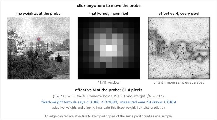
Strong or repeated filtering can flatten gradients into plateaus, retain isolated noisy pixels, or erase low-contrast texture. Similar edge-aware goals motivate anisotropic diffusion (Perona & Malik 1990), whose iterative update is a different operation.
Denoise color more than brightness⧉
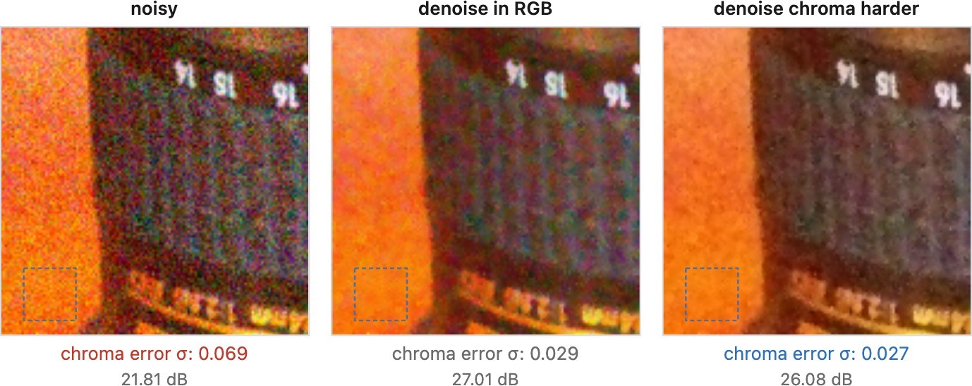
optionalVision generally resolves luminance detail more finely than chromatic detail. Many denoisers therefore smooth chroma more strongly. This is a tolerance, not permission to erase arbitrary color structure: isoluminant colored edges and fine saturated patterns can be visible.
A luminance/chrominance representation provides separate controls for brightness grain and color blotches. Stronger chroma smoothing can clean a neutral wall while retaining luminance texture; across colored boundaries it can bleed colors. RGB methods can also learn or implement such coupling. Choose the representation and weights for the image, rather than treating one channel layout as necessary for good denoising.
What each filter destroys⧉
optionalCompare results on flat regions, edges, and texture. Matching residual noise in a constant patch gives one useful operating point, but does not determine a universal ranking. An impulse-removal test and a Gaussian-noise test reward different behavior. Also inspect the removed signal $y-\hat x$: recognizable structures suggest lost detail, while their absence does not prove the estimate is correct.
Gaussian smoothing blurs boundaries. The median suppresses minority features along with outliers. The bilateral filter depends on contrasts being distinguishable from noise. These are consequences of the estimators, not parameters that can always be tuned away.
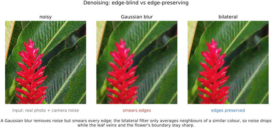
A larger neighborhood supplies more samples but may mix different scene values. Edge-aware and robust rules reduce some mixing errors; they do not establish that every retained feature is signal or every removed feature is noise.
With every filter of this chapter on the table, the most useful exercise is to run them against the same noisy image and watch the trade-offs move. The lab below splits one image into four panes, the split following the mouse, each pane with its own filter, its own sliders and its own live score (Figure 13.3.7). Put the Gaussian beside the bilateral and slide across an edge; set a pane to the amplified error against the clean original to see where each filter cheats, or to the difference of two panes to compare them directly.
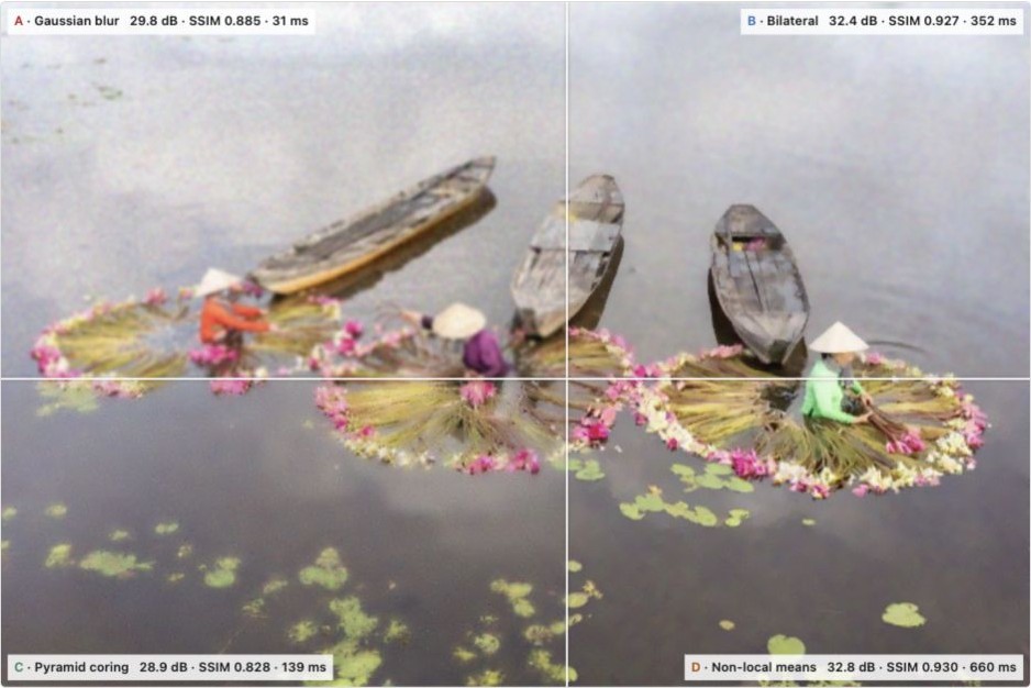
The limitation of a small window motivates the next methods. A faint texture may have too little evidence locally to distinguish it from noise. Multiscale methods look for related structure across scales; non-local methods search for repeated patches farther away; learned denoisers use regularities acquired from other images. Each broadens the evidence available to the estimate, while introducing its own assumptions about which structures should agree.
Non-local means and BM3D⧉
Non-local means: similarity as the weight⧉
optionalNon-local means (Buades et al. 2005) averages observed values with weights derived from patch similarity. One common version compensates for the expected noise contribution:
Here $S_p$ is a bounded search window and $h>0$ has the same intensity units as $\sigma$. The normalization by $m$ in the distance is essential: subtracting $2\sigma^2$ from an unnormalized sum would use the wrong noise scale. The subtraction and truncation are a practical weighting rule, not an unbiased estimator of similarity.
for p in image:
    w = empty_map()
    candidates = search_window(p) excluding p
    for q in candidates:
        d2 = mean((patch(y,p) - patch(y,q))**2)
        w[q] = exp(-max(d2 - 2*sigma**2, 0) / h**2)
    if candidates is empty:
        out[p] = y[p]
        continue
    w[p] = max(w[q] for q in candidates)
    if sum(w.values()) == 0:
        out[p] = y[p]
        continue
    out[p] = sum(w[q]*y[q] for q in candidates plus p) / sum(w.values())
This self-weight convention prevents an exact self-match from overwhelming much smaller neighboring weights. If the candidate set is empty or all weights underflow to zero, return $y_p$. Use a consistent boundary extension when extracting patches. For color images, distances can combine channels and the same weights can filter all channels, with the noise model adjusted for their variances and correlations.
Larger search windows cost more and offer more accidental matches as well as useful ones. Larger $h$ accepts less similar patches and smooths more strongly. Patchwise variants estimate whole patches and aggregate their overlaps. These details distinguish implementations of Chapter 10.2, Non-local means that otherwise share the same equation.
The method also carries a bias. It averages a patch with the patches that resemble it, so it pulls the image slightly toward its own repeated structures, and details with no match elsewhere, a crack in one brick, a single hair, get fewer effective samples and either stay noisy or are smoothed toward their nearest look-alikes. This is the first appearance of a failure mode that every method borrowing evidence from elsewhere in the image shares: good at what repeats, weaker at what does not.
The direct search repeats much of its arithmetic. For a fixed displacement, form an image of squared differences between the input and its shifted copy. A box sum, implemented with a summed-area table Crow 1984 or separable running sums, then gives all patch distances for that displacement. This reduces the cost of comparing large patches. A bounded search window limits the number of displacements; a pilot denoising pass can help select candidates, provided the final average still uses the intended measurements. These accelerations change different parts of the computation and can be combined.
BM3D: group, transform, shrink, aggregate⧉
optionalBM3D (Dabov et al. 2007) combines patch matching with Chapter 13.4, Pyramid and wavelet denoising. For each reference patch it selects similar patches, stacks them, applies a transform within each patch and along the stack, shrinks the coefficients, and transforms back. The third dimension indexes patches; it is not a spatial axis in the photograph.
If the patches were identical, an orthonormal transform along the stack with a constant first basis vector would concentrate their shared signal in that component. Real matches differ, so other components also contain signal. Shrinkage can retain these differences when they are sufficiently strong. It can also erase a genuine detail present in only one patch.
The method has two passes. The first uses hard thresholding and aggregates the reconstructed patches into a basic estimate. The second uses that estimate to select groups and estimate coefficient power, but filters groups extracted from the original noisy image. In a simplified orthonormal-transform description, its empirical Wiener gains are
A small pilot coefficient gives a small gain; a large one largely retains the noisy coefficient. With other transform normalizations, replace $\sigma^2$ by the appropriate coefficient noise variance. Group selection and overlapping samples make the actual statistics more complicated than this idealized expression.
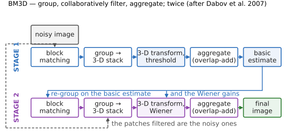
basic = aggregate(
    inverse_transform(hard_threshold(transform(group_from(y)), threshold))
    for each reference patch, with group matches found in y)

for each reference patch:
    positions = find_matches(basic)
    c_basic = transform(extract_group(basic, positions))
    c_noisy = transform(extract_group(y, positions))
    gains = abs(c_basic)**2 / (abs(c_basic)**2 + coefficient_noise_variance)
    accumulate(inverse_transform(gains * c_noisy), positions, group_weights)
out = accumulated_values / accumulated_weights
This outlines the data flow; a reproducible implementation must also specify transforms, matching thresholds, group sizes, spatial windows, and aggregation weights. Every reconstructed patch returns to its own original position. Overlapping estimates are combined with spatial and group reliability weights, then normalized. They share input pixels and are not independent new observations.
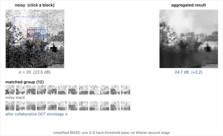
Suppose four matched patches were exactly equal except for independent noise. Along the stack dimension, their common component is constant, while their differences contain only noise. An orthonormal transform separates that constant direction from difference directions. Shrinking the latter suppresses disagreement while retaining the common patch. Real matches are only approximate: a small edge displacement or a texture difference can also occupy a difference direction. BM3D's grouping, shrinkage, and overlap aggregation must therefore balance agreement against genuine variation. This explains why grouping quality matters as much as the transform itself.
Learned denoisers⧉
optionalWavelet shrinkage assumes that useful image structure has a sparse representation. BM3D Dabov et al. 2007 searches for repetition within the observed photograph. A learned denoiser fits a mapping from noisy images to clean targets, using regularities across a training collection as well as spatial context within each input. Its behavior depends on the training images, corruption model, architecture, and loss.
For paired training with squared error, the ideal population solution is the posterior mean:
This characterizes an unrestricted optimum. Finite networks, finite data, and imperfect optimization only approximate it. A network can also be trained with another loss, in which case the optimal statistic changes. These distinctions matter when a trained denoiser is later interpreted as a score estimator in Chapter 13.11, Denoising as a universal prior.
Generative denoising with diffusion models⧉
optionalIn a very noisy photograph of a brick wall, several positions of a mortar line may be compatible with the measurement. Averaging those possibilities produces a softened edge. Choosing one produces a sharper edge whose position may be wrong. Generative denoising makes this choice explicit by producing plausible reconstructions conditioned on the noisy image.
The distinction matters where the observation leaves substantial uncertainty. It is not true that all posterior means look blurred or all posterior samples look realistic. Both depend on the scene, measurement, and learned distribution. A model that excludes the true structure can produce confident, consistent errors.
Denoising TLDR⧉
optionalFor ordinary photographic work, start with a pretrained denoiser designed for your input. The practical choices are what to capture, how much detail to retain, and how to judge the result.
- Preserve raw data when available. Match the denoiser to the camera data and processing domain it expects; a model for raw sensor noise and one for processed RGB solve different problems. In a custom pipeline, check black levels, image scaling, and noise units before tuning strength (Chapter 13.1, Noise models, transforms, and benchmarks).
- Use multiple frames when motion and capture time permit. Four aligned, independent exposures of unchanged duration halve noise standard deviation. Moving subjects and occlusions reduce that gain locally; splitting a fixed total exposure adds read noise. Use a temporal method for video and inspect ghosting, flicker, and delay (Chapter 13.2, Denoising by averaging, Chapter 13.10, Video denoising).
- Set strength by the detail you need to preserve. Inspect hair, foliage, fabric, small text, and isolated highlights at full resolution and at the intended display size. Some remaining grain is preferable to erased texture. More plausible texture from a generative method does not establish that the camera recorded it. Keep the original and record whether the output uses generative reconstruction (Chapter 13.9, Generative denoising with diffusion models).
- Test on your own images. Compare identical inputs, inspect the removed residual, and use reference error and perceptual measures when a reliable reference exists. Include difficult scenes and measure latency and memory. A benchmark winner may behave differently on your camera (Chapter 13.12, Measuring a denoiser).
- For implementation, use BM3D Dabov et al. 2007 as a baseline requiring no learned weights. Reserve median filtering for sparse impulses or defects; ordinary spatial smoothing also removes detail. Train a new model when available models fail your domain. Noisy-target training can help, but requires the independence and alignment assumptions developed in Chapter 13.8, Denoising without clean data.
Recap: big lessons in this lecture
Shot noise is Poisson, so its variance grows linearly with the signal ($\sigma^2 \propto N$) and its standard deviation grows only as the square root ($\sigma \propto \sqrt{N}$). Two consequences pull in opposite directions: the absolute noise is larger in highlights than in shadows (a 10,000-photon highlight has $\sigma=100$; a 100-photon shadow has $\sigma=10$), yet the SNR $= N/\sqrt{N} = \sqrt{N}$ is higher in the highlights: the signal outgrows the noise. So bright areas are noisier in absolute terms but cleaner to the eye; the shadows have the worst SNR (Figure 2.8.4, Figure 2.8.6). This is why exposing to the right and brighter scenes look smoother, and why we gamma/log-encode so equal ratios get equal steps.
Use the color / intensity difference between two pixels as how much they belong together, an affinity, then average (or connect) pixels in proportion to it. Pixels with high affinity are treated as measurements of the same underlying thing and get averaged together; pixels with low affinity, across an edge, are kept apart. The bilateral filter's range weight $g_r$ is the first full instance, but the same affinity drives the bilateral grid, the guided filter, non-local means (NL-means), colorization, and matting / segmentation that follow. Edge-preserving is affinity. (This is L10.1, registered in Part 13, Denoising where the bilateral first appeared for noise; this is its full edge-preserving treatment.)
Removing the bilateral normalizer changes the filter. Specify a normalized spatial kernel or an explicit step size, then test constants, impulses and edges. A small total affinity makes a small correction; it does not establish that an isolated value is correct.
Recording several captures lets us choose or combine their measurements afterward. A filter wheel is the plain example: shoot the scene through a red, a green and a blue filter (or through a polarizer at several angles) and the choice of how to combine the bands can be made later, at the desk. Exposure brackets, focal stacks, and panoramas extend this idea to different capture settings.
Several compatible measurements can reduce uncertainty or cover information missing from one frame. This is a different benefit from the previous lesson. Deferring a choice picks among things one exposure could have recorded; combining exposures can exceed what any single exposure could record, such as a noise level below one frame's, a dynamic range wider than the sensor's, or a depth of field deeper than the aperture allows. The reconstruction must account for differences in exposure, focus, viewpoint, or scene motion.
Averaging four independent measurements of the same signal halves the noise standard deviation. Averaging 100 reduces it by a factor of ten. These statements require zero-mean errors and unchanged per-frame variance. Lowering the effective noise floor can extend the usable range, as described in L2.46, provided the captures have not clipped the signal.
A larger neighborhood supplies more samples but may mix different scene values. Edge-aware and robust rules reduce some mixing errors; they do not establish that every retained feature is signal or every removed feature is noise.