Lecture Notes 0 — Intro⧉
Course notes cut from Computational Photography, an AI-powered Slopendium for this lecture. Each section links back to its home in the book; sections marked optional go beyond what the lecture needs.
Contents · 21 sections on this page, from 6 chapters of the book
Titles jump to the section below; ↗ opens it in the book.
From digital to computational photography⧉
A phone can combine several noisy exposures into one clear photograph, or use depth to blur the background behind a face. These pictures depend on both a physical measurement and a computation. Digital photography made that combination possible by recording the image as numbers; computational photography designs what we measure and how we turn those measurements into a picture.
Consider a dark room with a sunlit window. Exposures chosen for the room and for the view outside can be combined into a high-dynamic-range (HDR) image that retains both. Other methods estimate camera shake to reduce blur, stitch overlapping frames into a panorama, or record light from multiple viewpoints so we can refocus after capture. Each method uses additional measurements or assumptions. None can recover arbitrary information that the capture failed to record.
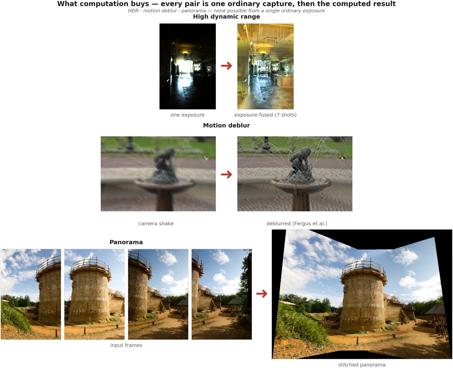
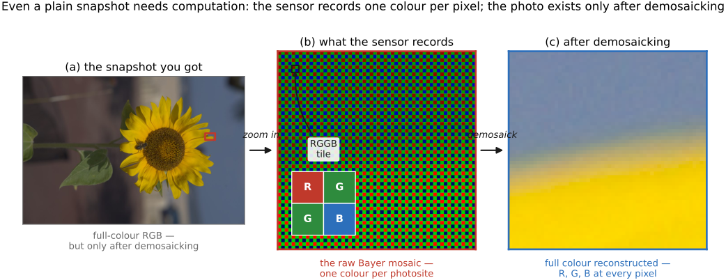
Even the most ordinary snapshot already depends on computation. As we'll see shortly, a typical sensor measures only one color channel at each pixel (red, or green, or blue), and the other two are reconstructed by an algorithm before you ever see a full-color image. Computation isn't an afterthought for fun special effects. It has become a fundamental aspect of image formation.
A phone has little room for a large aperture or sensor. Aligning and merging frames collects evidence over time, and denoising and tone reproduction help use that evidence. The small optics still matter: blur, flare, clipping, and motion can destroy information before processing begins. Computation and good hardware complement each other.
Generative models add another source of information: patterns learned from training images. They can synthesize or modify a picture, including details that the camera did not resolve. This makes restoration more flexible but raises a question that will recur throughout the book: which details are supported by the measurement, and which are plausible inventions? Borges's imagined library of every possible book offers an analogy for this breadth, but a learned model does not contain every possible photograph Borges 1941 Bottou & Schölkopf 2023.
Computation is the new optics⧉
In a conventional camera, the lens forms an optical image and film or a sensor records it. Better lenses, emulsions, sensors, and exposure control improve that measurement. Processing has always influenced the final photograph, including through chemical development and printing; computation greatly expands the operations we can apply.
Computational photography allows the final picture to differ substantially from the optical image. We can combine exposures, estimate missing values, and use measurements of depth or ray direction. The attainable result depends on the complete system: capture, reconstruction, and display.
The optical image need not look like the desired result. It can instead be designed to preserve information that an algorithm can recover. This is optics and computation co-design: choose the measurement and reconstruction together. A coded measurement is useful only if the desired information survives with enough signal relative to noise.
Consider extending depth of field. Wavefront coding Dowski & Cathey 1995 and the lattice-focal lens Levin et al. 2009 (4D frequency / lattice-focal) deliberately blur the optical image over a range of depths. They aim to make the blur more consistent and easier to invert than ordinary defocus, so one reconstruction can sharpen objects at different distances (Figure 1.1.3). In the usual incoherent imaging model, the sensor receives nonnegative sums of intensities; computation can also subtract and apply nonlinear operations. Deconvolution uses that freedom, at the cost of noise amplification and possible artifacts. The useful depth range and recoverable detail remain finite. See Part 33, Computational optics and coded imaging.
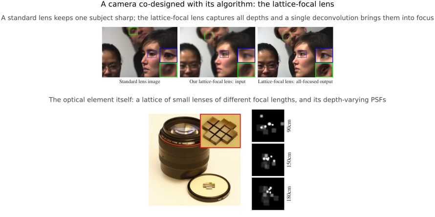
“Computation is the new optics” describes this expansion of image formation: we can improve the picture by changing the computation as well as the lens.
The goals of computational photography⧉
The methods in this book serve several photographic goals:
- Prettier pictures: straightforwardly better-looking results: cleaner, sharper, better-toned, more pleasing color.
- Alleviate physical limitations: reduce the effects of hardware constraints: too little light, too little dynamic range, a lens too small or too shaky.
- Record more information: capture what an ordinary photograph discards: depth, scene structure, separate layers of the scene.
- More control after capture: give the photographer more control after capture rather than locking in every decision at the moment of the shot.
- New visual experiences: make images that simply have no single-shot equivalent, like a refocusable photograph or a navigable panorama.
- Reveal the invisible: surface what the eye cannot see on its own, from tiny motions and color changes to information outside the visible band.
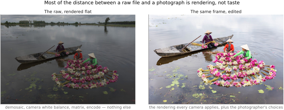
Prettier pictures. A raw file needs a rendering before it becomes a viewable photograph: white balance, color conversion, and a mapping to the display. A neutral rendering and a photographer's preferred rendering can look quite different (Figure 1.1.4). There is no single appearance intrinsic to the raw numbers.
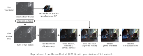
Alleviate physical limitations. A phone can merge a burst of short exposures, preserving highlights in each frame while reducing noise in the combined shadows. The additional frames collect more photons; alignment and merging make their measurements useful (Figure 17.6.6). Motion limits how much can be combined.
Record more information. Overlapping photographs can support a three-dimensional reconstruction and views from new camera positions (Figure 36.7.7). Coverage, texture, and scene motion determine which parts can be reconstructed reliably.
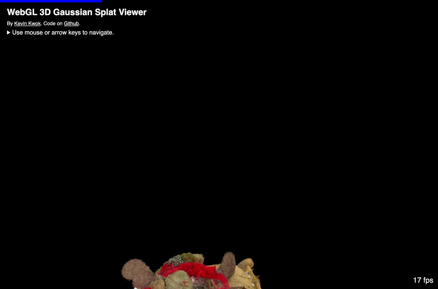
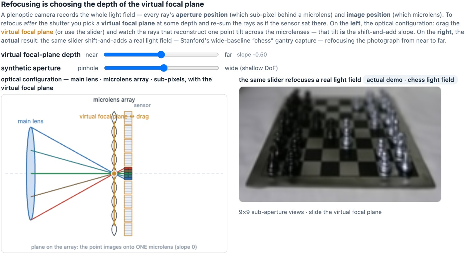
cakewalk/splat-data sample set (companion to the viewer). Viewer: antimatter15/splat (MIT).More control after capture. Recording ray direction as well as position allows refocusing within the range supported by the capture (Figure 31.4.2).
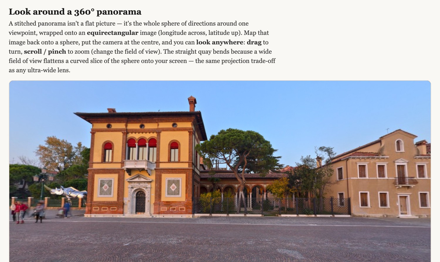
New visual experiences. Some images have no single-shot equivalent at all: you navigate them rather than look at them (Figure 20.4.5).
Reveal the invisible. The camera had already recorded a face flushing with its pulse and a building swaying. What was missing was the processing that makes such changes visible.
A limitation can also be an expressive choice (Figure 1.1.5). Leaving deep shadows black may make the lit shapes easier to read than opening every shadow. Freezing a fraction of a second lets us study a gesture that passed too quickly to see. More recovered detail is not always a better photograph.
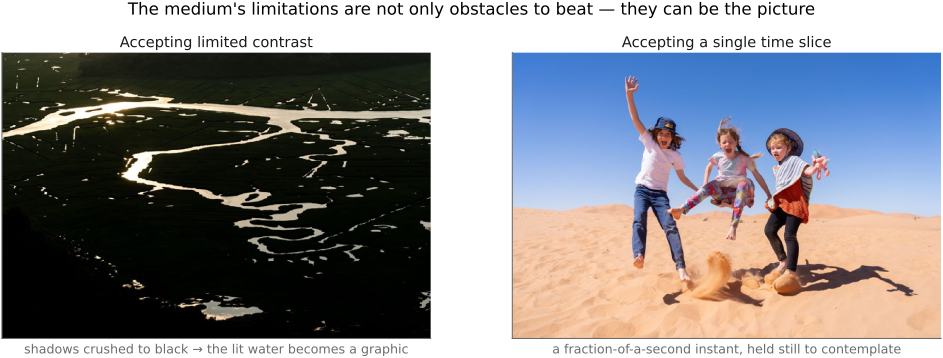
The intended use determines how we evaluate an image. A calibrated measurement can be assessed against a physical quantity, with uncertainty attached. A perceptual model predicts visibility or appearance under specified viewing conditions. A photographer may instead choose a rendering for its expressive effect.
These criteria can disagree. Smoothing a face may reduce pixel error while removing texture the photographer wants. Preserving every shadow detail can flatten the composition. Human vision has measurable regularities, including contrast sensitivity and color matching, but perceptual metrics remain models with limited ranges of validity. Choose the criterion before comparing methods.
Between physical measurement and personal preference lies perceptual vision, which concerns how an image actually looks to a human eye. You might expect this to be hopelessly subjective, but it is not. Several aspects of human vision can be modeled quantitatively: the contrast sensitivity function, color appearance, lightness and brightness, visual masking, perceived sharpness, and full image-quality metrics such as SSIM and visible-difference predictors. "How it looks" can be measured and even predicted, though it is not pure physics. Within a model’s range of validity, this lets us engineer for the eye: tone-mapping to fit the eye's response, throwing away color detail the eye won't miss, choosing where to spend bits or where a little smoothing will go unnoticed.
Hand-designed algorithms, learning, and generative AI⧉
optionalHand-designed methods specify how to reconstruct an image. Learned restoration estimates that mapping from examples. Generative methods learn a distribution of images and can sample possible outputs, often conditioned on a capture. These approaches coexist: a camera may use a conventional geometric alignment stage, a learned denoiser, and a hand-designed tone curve.
The distinction does not by itself tell us how faithfully a result follows the data. A hand-designed prior can erase real texture; a learned model can be constrained by the measurement. Generative restoration is especially useful when many plausible images explain the input, but the selected detail need not be the detail that was actually there. Evaluation must reflect whether the task is measurement, photographic rendering, or synthesis.
Rich Sutton's The Bitter Lesson argues that general methods able to exploit growing computation tend to outperform elaborate hand-coded knowledge over time. Natural-language processing gives the standard example. For decades, parsing a sentence meant hand-building grammars that encoded linguists' knowledge of syntax; statistical parsers trained on corpora of annotated sentences overtook them, and neural models later did so with still less hand-designed structure. The linguistic knowledge did not stop being true. It stopped being the thing programmers wrote down directly, and moved into the data, the annotations and the choice of what to measure. Imaging offers an important place for physical knowledge within learned methods: we can model projection, blur, sensor noise, and the color-filter mosaic to generate training pairs or constrain reconstruction. Those pairs are exact for the simulator, not necessarily for a real camera. Calibration errors, clipping, motion, and unmodeled processing can make synthetic training data misleading. Chapter 7.2, Machine learning and Chapter 7.3, Deep learning develop these approaches.
Photography developed through advances in optics, chemistry, electronics, and computation. Selected milestones:
- Optics first: the camera obscura. A darkened room or box with a small hole projects an inverted image of the world onto the far wall, the ancestor of every camera. Known since antiquity, described carefully by Alhazen around 1020, and used as a drawing aid by Renaissance painters: image formation centuries before anyone could fix the image in place.
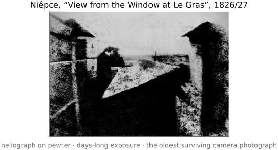
- 1826/27: an early camera photograph. Nicéphore Niépce records a lasting image by heliography, the oldest surviving photograph made in a camera (Figure 1.1.6).
- 1839 / 1841: public photographic processes. Daguerre's daguerreotype was announced in 1839. Talbot's calotype, patented in 1841, used a paper negative from which multiple positive prints could be made. Science Museum Group.
- 1839: an early self-portrait. Robert Cornelius made a daguerreotype self-portrait in Philadelphia, cataloged as the earliest surviving American portrait photograph by the Library of Congress.
- 1851: wet collodion. Frederick Scott Archer's collodion process cuts exposure times to a few seconds.
- 1861: three-color photography. James Clerk Maxwell combines three exposures through red, green, and blue filters, the three-channel idea we still use.
- 1871 / 1888–89: the introduction of film. Richard Maddox's gelatin dry plate (1871) lets the light-sensitive emulsion be manufactured in advance, instead of coated wet on a glass plate on the spot. George Eastman then replaces the glass entirely with a flexible, rollable emulsion: paper-backed roll film (1888) and then a transparent celluloid base (1889). This flexible strip is film in the literal sense, and it would remain the medium of photography for the next century, until digital capture became widespread.
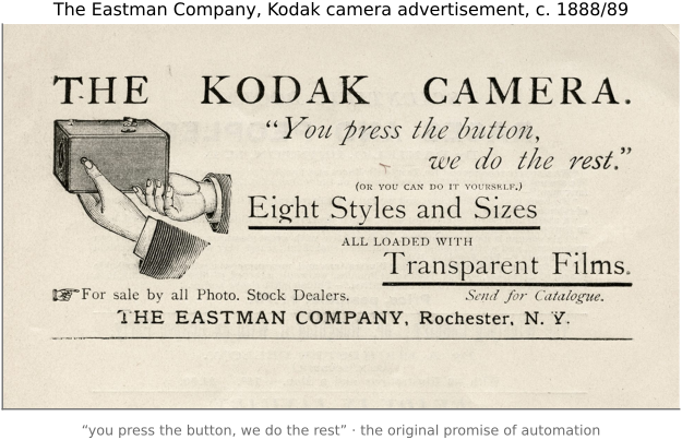
- 1888 / 1900: photography for everyone. Kodak's roll film arrives under the slogan "you press the button, we do the rest" (1888); the Brownie (1900) puts a camera in ordinary hands. As Peyman Milanfar points out, that advertising line is already the thesis of this whole book: the photographer presses the button and something else does the rest; computational photography is simply the modern answer to what "the rest" is and how much of it can be done (Figure 1.1.7). In parallel, the Lumière brothers launch cinema (1895) and a practical color process, Autochrome (1907).
- 1925: the Leica. 35 mm becomes the standard small format.
- 1935: coatings and color film. Anti-reflection lens coating (Smakula, at Zeiss) cuts internal flare and lifts transmission and contrast, later refined into multi-coating, like Zeiss's T*, in the 1970s. The same year, Kodachrome delivers practical color film (Kodacolor color-negative film follows in 1942).
- 1948: instant photography. Edwin Land's Polaroid Land Camera develops the print inside the camera in about a minute, no lab, no waiting; the iconic folding SX-70 single-lens reflex follows in 1972.
- 1963: simpler loading. Kodak's Instamatic, with its drop-in cartridge, simplifies loading and cements the mass-market snapshot.
- 1969 / 1975: toward digital. Boyle and Smith invent the charge-coupled device (CCD) (1969); Steven Sasson at Kodak builds the first digital-camera prototype around one (1975).
- 1993: the CMOS active-pixel sensor. Eric Fossum and colleagues at NASA's Jet Propulsion Laboratory develop the CMOS active-pixel sensor (APS), putting an amplifier at every pixel on an ordinary CMOS process Fossum 1993. Cheaper to make, lower-power, and faster to read out than the CCD, and able to integrate logic on the same chip, it eventually displaced the CCD almost everywhere and became the sensor in essentially every phone and most cameras: the device that made on-device computational photography practical at scale.
- 1977 / 1985 / 1995: automation. The Konica C35 AF (1977) and Minolta Maxxum 7000 (1985) mark the spread of autofocus. Canon's EF 75–300mm IS USM (1995) brought optical stabilization to an EF lens; sensor-shift stabilization later provided another way to compensate for camera motion.
- Late 1980s–1990s: the image industry went digital before the camera did. Long before most photographs were captured digitally, the photo industry had already moved to digital images. Desktop publishing and digital prepress (late 1980s) scanned film for page layout; drum and film scanners, together with Kodak's Photo CD (1992), digitized negatives and slides; Adobe Photoshop 1.0 (1990, the Knoll brothers, Thomas and John) put the darkroom on a desktop; and photojournalism digitized early, with Kodak DCS bodies feeding pictures down the wire, because filing a picture fast beat film's quality. Images were edited, scanned, and transmitted digitally years before the camera itself caught up.
- 1990s / ~2000: the digital era. The first practical digital cameras appear through the 1990s, the Kodak DCS (1991), the Apple QuickTake (1994), and the Nikon D1 (1999), and camera phones follow around 2000, putting a camera in every pocket.
- ~2002: the picture becomes a message. The Multimedia Messaging Service (MMS) extends the plain text message to carry a photo, so a camera-phone snapshot can be sent the instant it is taken. Together with the new camera phones, it quietly changes what a photograph is for: no longer something you develop and later show, but something you transmit immediately, the first sign that a picture's destination is now another screen, seconds away.
- 2000s–2010s: digital replaces film in many applications. Resolution, high-ISO performance, dynamic range, and delivery speed improved substantially. Comparisons depend on film stock, format, scanning, and the metric; there is no universal crossover year.
- 2000s–2010s: front-facing and multiple rear cameras. Front-facing cameras supported video calls and self-portraits. Multiple rear cameras with different focal lengths, as in the iPhone 7 Plus (2016), extended the useful zoom range and supplied additional measurements for computational imaging.
- 2004 / 2010: photography becomes social. Facebook (2004) and then Instagram (2010) make sharing the point of taking a picture: billions of photos are uploaded and seen by others within seconds of capture. Instagram's one-tap filters also put a computational look on every image, normalizing the idea that a snapshot is processed before anyone sees it, and the feed turns the photograph into a unit of social communication as much as a keepsake, the demand side of the phone-camera explosion, and the reason "how it looks on a small screen, right now" became a design target.
- 2012 / ~2014 / ~2022: the learning era. ImageNet and AlexNet set off the deep-learning revolution in vision (2012); generative adversarial networks (GANs) arrive in 2014; diffusion models and systems like DALL·E bring generative image AI into the mainstream around 2022.
- Other side branches. The flash, which let photographers carry their own light; holography, which records the wavefront itself rather than a flat image; Gabriel Lippmann's integral imaging and his interference-based color photography; consumer light-field cameras like Lytro; and the term "computational photography" itself, coined by Steve Mann in the mid-1990s and broadened into common use by Marc Levoy in the mid-2000s.
Consider just how little the first digital cameras could do; it sets the baseline everything in this book improves on. Two machines bracket the start of the era, one professional and one consumer:
- Kodak DCS-100 (1991): the first commercial digital SLR. A stock Nikon F3 film body was mated to a Kodak 1.3-megapixel CCD ($1024\times1280$), but the camera could not stand alone: it was tethered by cable to a separate, shoulder-slung Digital Storage Unit, a box holding a 200 MB hard drive, batteries, and a tiny monochrome preview screen, that stored roughly 150–600 images per session. Sensitivity ran about ISO 100–400 (a monochrome version reached higher). Price: around \$20,000–\$25,000. It existed for one reason: photojournalists could wire a picture to the newsroom in minutes instead of shipping film.
- Logitech Fotoman (1992): a rebadged Dycam Model 1 (1990), one of the first fully self-contained consumer digital cameras. It shot 376×240 pixels in 8-bit grayscale (256 levels), held about 32 images in 1 MB of internal RAM (lost if the batteries died), had a fixed-focus lens and a built-in flash, and downloaded over a serial cable to a PC or Mac. Price: around \$600–1000. No color, no screen, about 0.09 megapixels in monochrome, and still a glimpse of the future.
Put beside a modern phone (tens of megapixels, color, video, and a stack of computation behind every frame), these are strikingly limited. The improvement reflects both better sensors and more capable processing.
This also changes an expectation that developed around photographs. Perspective construction, photographic capture, and documentary practice all helped establish the image as evidence about a particular scene. Photojournalism gave special importance to the idea of recording an actual instant. That ideal was never a complete description of image-making: staging, framing, and manipulation remained. Generative synthesis makes the distinction especially visible because a convincing image need not originate in a corresponding event. The question is what relationship to an event a viewer is entitled to expect.
The physical knowledge accumulated in imaging still has work to do. A hand-designed denoiser puts assumptions directly into its algorithm; a learned denoiser can inherit them through simulated noisy/clean pairs, its architecture, or a measurement constraint. Knowledge of the camera has moved into a different part of the design. The practical question is where that knowledge is most useful, and how closely the simulated measurements represent the real capture.
A multidisciplinary field⧉
optionalComputational photography draws on optics and sensor engineering to form measurements, algorithms and machine learning to reconstruct images, and perception and photographic practice to judge the result. Performance engineering determines what can run on a device. Ethics matters when the processing changes how we represent a person or an event.
A few neighboring fields overlap with computational photography so heavily that it helps to say exactly how they relate and differ.
Computer vision is the closest. A useful way to carve up vision is by its three ingredients: 2-D images (the pixels themselves: filtering, features, matching), 3-D (the geometry behind the pixels: depth, shape, pose), and meaning (semantics: what objects and scenes the pixels depict). Computer vision ultimately cares most about the last two: it treats the image as a means to recover 3-D structure or to understand content. Computational photography inverts that emphasis: its product is the 2-D image, a better photograph. But it freely reaches into 3-D and meaning when they help the picture: depth to fake a shallow-focus background, segmentation to brighten a face and not the sky, recognition to pick the frame where everyone is smiling. The same tools, pointed at a different goal.
Computer graphics runs the arrow the other way, synthesizing images from models of geometry, materials, and light. Computational photography borrows its rendering and image-based-rendering machinery (and, increasingly, shares it outright: gradient-domain editing, light fields, differentiable and neural rendering all live in both). Image processing is the classical signal-processing bedrock the whole enterprise is built on: filtering, transforms, sampling, and compression. Models of capture help choose the processing. And optics supplies the physics of image formation, which computational photography increasingly co-designs with the computation rather than treating as fixed (coded apertures, lensless cameras, end-to-end optimized lenses).
Because the field straddles these neighbors, so does its literature. A great deal of computational photography is published at the major computer-vision conferences (CVPR, ICCV, and ECCV) and at the graphics venue, SIGGRAPH (and SIGGRAPH Asia / ACM Transactions on Graphics). ICCP, the IEEE International Conference on Computational Photography, is a venue dedicated to the field.
These disciplines appear together inside a single feature. Take a phone's night mode. It leans on physics (catching scarce photons), electrical engineering (the sensor that catches them), algorithms (aligning and merging a burst of frames), AI (learned denoising), perception (tone-mapping the result so it reads naturally), performance engineering (finishing within a short capture budget on a phone without excessive energy use), and ethics (how much to "beautify" a face, and whether to tell the user), all at once. Each discipline constrains the others: a more expensive reconstruction can require fewer input frames or a longer wait for the picture.
Beyond photography⧉
The methods used on photographs also apply to other measurements. The shared approach is to specify what an instrument records and reconstruct the quantity we want from it.
Start with the ordinary camera pointed at extraordinary jobs. The instant a camera stops being aimed by a human enjoying the view and starts being aimed by a machine making a decision, the processing serves a different task. Robotics and self-driving cars lean on cameras (and their cousins, depth sensors and lidar) to perceive, localize, and navigate. The alignment, depth, and motion estimation we develop for panoramas and refocusing are exactly what a robot needs to know where it is and what is moving. Surveillance and security, industrial inspection (spotting a hairline crack or a misplaced solder joint on a production line, where consistent lighting and repeatable measurements help detect defects), agriculture, drones, document scanning, and biometrics all use computational imaging for practical tasks. The picture is no longer the product; it is an input to a decision.
Then push the optics past what a handheld lens can do. Astronomy is computational photography at the grandest scale: telescopes stack thousands of frames to beat noise (the same averaging that powers a phone's night mode), use adaptive optics to cancel the atmosphere's blur in real time, and combine separate dishes into one synthetic aperture, the trick that let the Event Horizon Telescope assemble an Earth-sized virtual lens to image a black hole. At the opposite scale, microscopy does the same: light-sheet, confocal, and computational microscopes reconstruct 3D cellular structure, and super-resolution techniques reach past the diffraction limit we will meet in the optics part. Both require designing the measurement and reconstruction together.
Change the wavelength and the field opens again. Visible light is a sliver of the electromagnetic spectrum, and imaging lives all along it. Infrared gives thermal cameras and night vision; ultraviolet reveals forgeries and surface detail; X-ray imaging, in the form of computed tomography (CT), reconstructs slices or volumes from X-ray attenuation measurements along many paths, a reconstruction problem; radio gives us radio astronomy and synthetic-aperture radar (SAR) that maps terrain through clouds and darkness. Much of medical imaging is this same discipline under a different name: CT, magnetic resonance imaging (MRI), positron-emission tomography (PET), and ultrasound are all reconstruction problems, recovering an image from indirect measurements using related reconstruction ideas, including the regularized inverse problems this book builds up to. A radiologist's scanner and a phone's night mode use closely related reconstruction ideas.
And the techniques do not even need an image at all. Sampling, filtering, the Fourier transform, denoising, priors, inverse problems. The toolkit is really a toolkit for signals, and a signal can be anything. Audio is the obvious neighbor: a sound is a one-dimensional signal, and the same spectral and statistical ideas drive noise reduction, compression, and synthesis there. One example shows the connection: Paul Lamere's Infinite Jukebox takes a song, finds beats that sound nearly identical, and quietly jumps between them to extend the track, with success depending on the available transitions, which is precisely the idea of Video Textures (Schödl et al. 2000), a computational-video technique that finds similar frames in a short clip and loops between them to synthesize a video of arbitrary duration with varied transitions, transplanted from pictures to sound.
Run the trade the other way, too: point a camera at a quantity that has nothing to do with light and let computation read it out. Two examples make the point. GelSight turns a camera into a sense of touch: press a slab of clear elastomer, with its outer face painted with an opaque membrane, against an object, and the gel molds to the surface's microscopic relief; a small camera behind the gel photographs that deformation under raking colored light and reconstructs a dense 3-D height map by photometric stereo. Its resolution depends on the optics, camera sampling, illumination, and mechanics of the membrane. It can read the ink of a banknote, the wear on a machined part, and the grain of a fingerprint, and it has become a workhorse for robotic manipulation, where a gripper needs to feel contact, slip, and texture, right down to vision-based tactile sensors built into the fingers of a dexterous robot hand Romero et al. 2024 (EyeSight Hand). Touch becomes an image that can be analyzed with image-processing tools Johnson & Adelson 2009. The second example points a camera at vibration: ordinary objects tremble by thousandths of a pixel in response to sound and force, and that motion, amplified and demodulated, turns a silent video into a measurement of the world's movement. A bag of chips behind soundproof glass becomes a microphone. The visual microphone recovers intelligible speech from the sub-pixel wobble of its surface Davis et al. 2014; the same sub-pixel motion, read as a modal signature, recovers an object's material properties Davis et al. 2015 and lets a single camera perform structural health monitoring of a bridge or a building, identifying its resonant frequencies and mode shapes from across the street Chen et al. 2015 Davis 2019. We return to both threads in Part 38, Revealing the invisible; these examples show how images can serve as measurements of other quantities. Touch and vibration are signals, and a camera plus computation is a remarkably general instrument for measuring them.
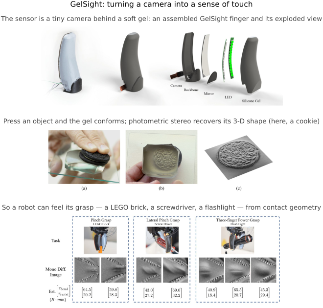
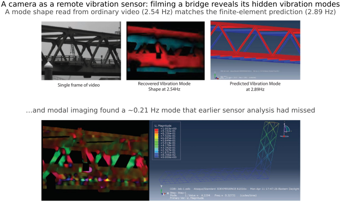
Many sensors make a quantity visible indirectly. Fluorescent markers emit light; an elastomer deforms under pressure; scintillators convert absorbed X-rays or gamma rays into visible light. A camera then turns that light into electrical measurements. In a semiconductor photosite, absorbed photons can generate electron–hole pairs whose charge is collected. This conversion, described in Chapter 2.7, Sensors: photosites, CCD vs CMOS, is one useful transduction mechanism among many, including the acoustic measurements used in ultrasound.
Part 39, Adjacent fields and applications develops these connections across imaging instruments and other signals.
The optical readout is often a design choice. We can arrange for pressure to deform a visible surface, for a chemical marker to fluoresce, or for an absorbed X-ray to produce a visible flash. Once the quantity modulates light, photodetection converts it into an electrical signal that familiar acquisition hardware can record. This is why an imaging course can teach useful measurement ideas far beyond cameras. We still have to model the conversion from the original quantity to light; linearity of the final sensor does not make every earlier conversion linear.
What programming language for computational photography?⧉
Use Python to learn the algorithms and explore images. Its array and machine-learning libraries perform their expensive operations in compiled code, often on a GPU. Use C++ or Halide when you need more control over an imaging pipeline's runtime and memory. JavaScript and WebAssembly provide a way to deliver interactive tools in a browser; phone applications also need platform-specific capture APIs.
The book provides Python and C++ implementations of the same ideas. A language does not determine speed by itself. In the course, replacing naive Python pixel loops with optimized compiled code sometimes produced speedups near 1000×. Such a comparison measures implementation choices as well as language: array operations, fusion, memory layout, and parallelism matter. Measure the complete pipeline, including image transfers and startup, before choosing what to optimize (Part 29, Making computational photography code fast).
On the desktop: Python, C++, and Halide⧉
Python is a convenient default for numerical experiments. NumPy represents images as arrays, while PyTorch and JAX add GPU computation and automatic differentiation. A per-pixel loop in Python can be slow; an array expression delegates the loop to compiled code. Vectorization can also create large temporary arrays, so memory traffic still matters. In conventional CPython builds, the global interpreter lock limits simultaneous execution of Python bytecode; compiled libraries can release it, and optional free-threaded builds have different behavior. Check the interpreter and extensions you deploy (Python documentation).
C++ offers explicit control of data layout, allocation, and parallel execution. That is useful for a pipeline with a tight latency or memory budget, but it requires more care with indexing, ownership, and build configuration. Standard containers and resource-owning objects reduce the need for manual allocation. Static types catch some errors; they do not catch a wrong color space or an out-of-bounds access automatically.
Halide separates an image-processing algorithm from its schedule: where and in what order values are computed, stored, vectorized, and parallelized. This lets the same algorithm support several execution strategies without rewriting its mathematical definition. Good schedules can avoid intermediate images and repeated memory transfers. They do not guarantee a fixed speedup over well-optimized C++ (Halide).
In 2013 Adobe, through the Computer History Museum, released the source of Photoshop 1.0.1: about 128,000 lines in 179 files, written for the original Macintosh largely by Thomas Knoll. Roughly three quarters is Pascal, the productive high-level language for the bulk of the program, and about 15% is hand-written 68000 assembly for the speed-critical inner loops. That is the split this chapter keeps returning to, thirty-five years early: hand-tune the hot pixel loops and keep the rest readable, the same trade as Python calling a compiled library, with a person doing by hand what Halide now automates. The code is now read as a cultural text too: the German research program Das digitale Bild (DFG, LMU Munich) has published a critical code study, reading the Photoshop source the way one close-reads a document (Reading the source code for Adobe Photoshop). The appendix runs the program itself (Chapter 45.33, Photoshop 1.0, running), and Part 29, Making computational photography code fast returns to hand-tuned inner loops.
Much of the computational-photography literature was prototyped in MATLAB. For years it was the platform for this kind of work: a strong numerical and linear-algebra library, and an interactive IDE that could read, display, and manipulate images natively: an image was just a matrix, imread/imshow and array slicing made experiments effortless, and the Image Processing Toolbox supplied the rest. NumPy carries the same array-as-image approach into Python, while frameworks such as PyTorch combine tensor operations with automatic differentiation and GPU execution. We mention it because older papers and code you will meet are written in it, and the array-thinking it taught carries over directly to NumPy. Choose the environment that lets you reproduce and inspect a method, rather than translating working research code only for consistency of language.
For example, NumPy's out = a + 0.5*b makes a point operation almost as direct to write as its mathematical definition. That short edit-and-run cycle matters when the algorithm itself is uncertain. Once the operation is settled, C++ can give more control over storage and execution, with a heavier build cycle and more responsibility for object lifetimes. Halide adds a scheduling language when the performance question is where to compute and retain intermediate values. These are different costs to pay at different stages of a project.
Vibe coding⧉
optionalAn LLM can help draft image I/O, visualizations, and numerical functions. Check the result against inputs with known answers: a constant for normalization, an impulse for a filter kernel, or a half-plane for resampling. A plausible photograph can conceal a wrong transfer function, offset, or boundary rule. See Chapter 9.1, Developing, Testing and Debugging.
The failures are not confined to difficult algorithms. While reproducing Photobios, the morphing slideshow that ages a person across a photo collection (Part 28, Photo collections), the coding agent handled face alignment and a dynamic-programming path through the images, then repeatedly got the cross-fade wrong. It took about five re-prompts to correct it. The intended operation was:
# start and end: aligned float images in the same chosen color representation
# t: blend fraction between 0 and 1
frame = (1 - t) * start + t * end
At zero the output must equal the start image, at one it must equal the end image, and equal inputs must remain unchanged. These simple checks establish properties that visual plausibility alone does not.
The book's interactive figures were developed with coding agents and often needed several rounds of correction. Review the computation and the displayed result together: a correct kernel can still be shown with the wrong range or encoding. A model's explanation of its code is not an independent check of that code.
Problem sets⧉
Implementing a method exposes choices that an explanation can hide: boundary handling, units, numerical precision, and failure cases. These assignments from MIT's Digital & Computational Photography course ask you to build simplified algorithms and try them on real photographs. Their sequence follows the course rather than the book; each assignment links to the chapters it uses. Full handouts are collected in Part 45, Appendices.
Start with small inputs you can check by hand, then inspect the photographic results. A constant image, an impulse, or a known geometric transform often reveals an error more clearly than a natural photograph. If you are taking a course, follow its own submission and AI-assistance rules.
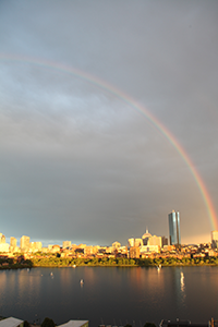 PS0: Environment and C++ basics. Set up the toolchain, write a minimal
Imageclass, and read and write image files. (→ Chapter 9.1, Developing, Testing and Debugging)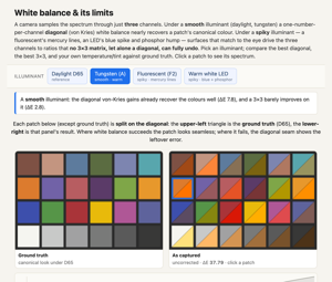 PS1: Image class, point operations, color. Pixel access; brightness and contrast; the luminance–chrominance (YUV) split; gamma; white balance; and the Spanish-Castle afterimage illusion. (→ Chapter 8.1, Image representation, Chapter 8.3, Tone point operations, Chapter 3.2, Perceptual color and trichromatic vision)
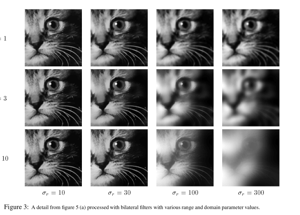 PS2: Convolution and the bilateral filter. Box and Gaussian blur, image gradients, sharpening, and bilateral denoising (with a YUV chroma variant). (→ Chapter 6.2, Convolution, Chapter 10.1, Bilateral filtering)
 PS3: Denoising and demosaicking. Align-and-average a burst (and the ISO/variance story); Bayer demosaicking: basic green, then edge-directed green and color-difference R/B; and Prokudin-Gorsky three-plate color alignment. (→ Part 13, Denoising, Part 15, Demosaicking and joint methods)
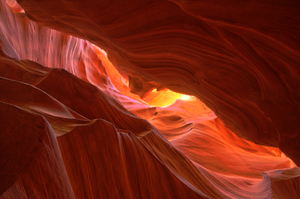 PS4: High dynamic range. Merge an exposure bracket into a radiance map and tone-map it for display. (→ HDR merging, Chapter 18.2, Global tone mapping)
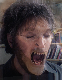 PS5: Resampling, warping, and morphing. Nearest / bilinear / bicubic / Lanczos resampling; Beier–Neely segment warps; and a full Beier–Neely morph. (→ Chapter 11.1, Warping, Chapter 11.3, Morphing)
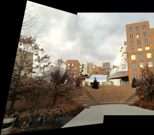 PS6: Homographies and manual panoramas. Homogeneous coordinates, warping by a homography, solving the homography from four point correspondences, and stitching a planar mosaic. (→ Chapter 20.1, Manual panorama stitching from multiple views)
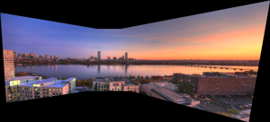 PS7: Automatic panoramas. Harris corners (the structure tensor), patch descriptors, the second-nearest-neighbor ratio test, RANSAC, and feathered / two-scale blending. (→ Chapter 20.2, Automatic panorama stitching from multiple views and feature matching)
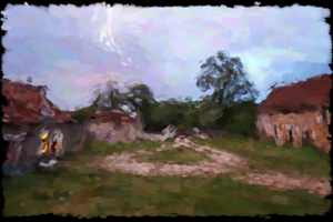 PS8: Non-photorealistic rendering. Paintbrush splatting and single-scale, two-scale, and gradient-oriented painterly rendering. (→ Chapter 25.2, Non-photorealistic rendering)
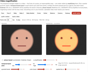 PS9: Make-your-own, video, and ethics. A self-proposed project (optical-flow retiming, phase-based video magnification, and the like) together with the ethics deliverable. Its open menu of advanced topics seeds many sections of Part 33, Computational optics and coded imaging. (→ Chapter 12.8, Optical flow, Chapter 38.3, Motion and video magnification)
The assignments deliberately distill an area into a small algorithm that you can build and inspect. Their purpose is to expose the principle before the production machinery obscures it. A basic align-and-average burst, for example, makes registration and noise reduction visible even though a shipping camera will need more elaborate handling of motion and outliers.
Image representation⧉
An image is an array⧉
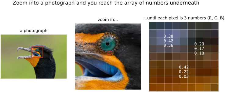
optionalA color image is stored as a grid of channel values, commonly red, green, and blue (Figure 8.1.1). These are samples or measurements; drawing enlarged pixels as squares is a display convention, not a complete model of sensor integration.
More formally, an image is a function defined over a 2-D domain, the grid of integer positions $(x, y)$, whose values live in a range, here the space of colors. We store that function as a three-dimensional array of size $\text{height} \times \text{width} \times \text{channels}$ and write $I(x, y, c)$ for the value at column $x$, row $y$, channel $c$. A grayscale image has a single channel, and we drop the index and write $I(x, y)$.
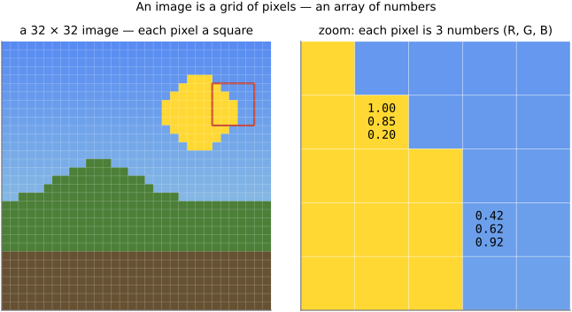
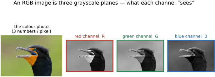
Usually a pixel carries exactly three channels, but nothing forces that. Some images add a fourth (for transparency, which we return to under alpha below) and scientific hyperspectral images keep dozens or hundreds of narrow wavelength bands instead of three broad ones. One very practical trap follows from this freedom, and it bites beginners constantly: a Portable Network Graphics (PNG) file may carry an alpha channel, so a file you assume is three-channel RGB hands you four channels instead. If the rest of your code expects three, every pixel downstream is misread. The fix is trivial once you know to look (check the channel count on load), but the symptom (colors scrambled, code not crashing) is hard to diagnose if you do not.
We use float32 for working images. Zero and one serve as black and reference white in normalized examples, but intermediate values may lie outside that interval. Changing an integer array to float changes its numeric representation; it does not decode its transfer function or identify its color space.
How the array sits in memory⧉
optionalThe array is two- or three-dimensional, but computer memory is one long line of numbered addresses. Something has to decide how the grid gets flattened into that line, and there is no single right answer. Different ecosystems made different choices, which matters the instant you pass an image between them.
The examples use packed planar C++ storage and HWC Python arrays. In contiguous planar storage, the element offset is $cWH+yW+x$; in contiguous interleaved storage, it is $(yW+x)C+c$ (Figure 8.1.6). A NumPy array can have other strides after slicing or transposition, and tensor dimension order does not uniquely determine physical memory layout. Query shape, strides, and contiguity at library boundaries. Row strides are $W$ elements per planar channel or $WC$ elements for interleaved RGB, before padding; byte strides also include element size.
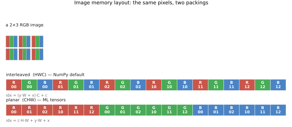
R G B R G B … row by row; pixel $(x, y, c)$ is at offset $(y\cdot W + x)\cdot C + c$. Planar (CHW): all of the red channel, then all of green, then all of blue, three contiguous planes; pixel $(x, y, c)$ is at offset $c\cdot W\cdot H + y\cdot W + x$. Same numbers, same picture; only the walk order through memory differs.The second decision is the order within a pixel. Most of the world, and this book, store the channels as red, green, blue (RGB), but a few libraries, OpenCV being the notorious one, use BGR. Mix the two and red and blue swap silently: skies turn orange, skin turns blue, and nothing throws an error. So always know which order your data is in.
Why care about any of this for everyday code? Mostly you should not. The mental model is just "a grid of pixels," and the accessor we build below hides the packing entirely. Two situations force you to think about it: performance (a loop that strides through memory in contiguous order runs far faster than one that hops around, so the right layout for an algorithm matters when speed does), and interoperability (handing an image to a library that expects a different layout means rearranging the array first). Outside those, the packing is an implementation detail.
Walking contiguous elements usually makes better use of cache lines and vector instructions. For packed HWC data, scalar loops run y, then x, then c; for planar CHW, c, then y, then x. A kernel that processes one whole pixel at once can hide the channel loop. Tiling, vectorization, compiler transformations, and hardware affect the best schedule; measure the implementation (Figure 8.1.7).
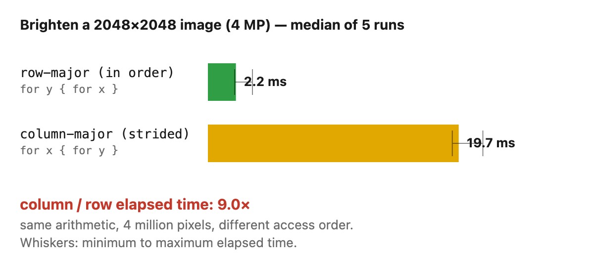
for y { for x } and the cache-hostile for x { for y }, warms up the JIT, then times several passes of each and reports the medians with their min–max spread. The arithmetic and the pixel count are identical; only the memory access order differs, yet the column-major walk typically runs several times slower on the very machine you are reading this on. Interactive: press Run to re-measure, and change the image size; watch the column-major bar stay several times longer than the row-major one, with tight whiskers showing the measurement is stable.Planar storage makes same-channel values contiguous. Interleaving keeps all channels of each pixel together, which can help operations that use them jointly. Vector implementations can handle either layout. Conversion costs and the whole pipeline matter more than declaring one layout universally faster.
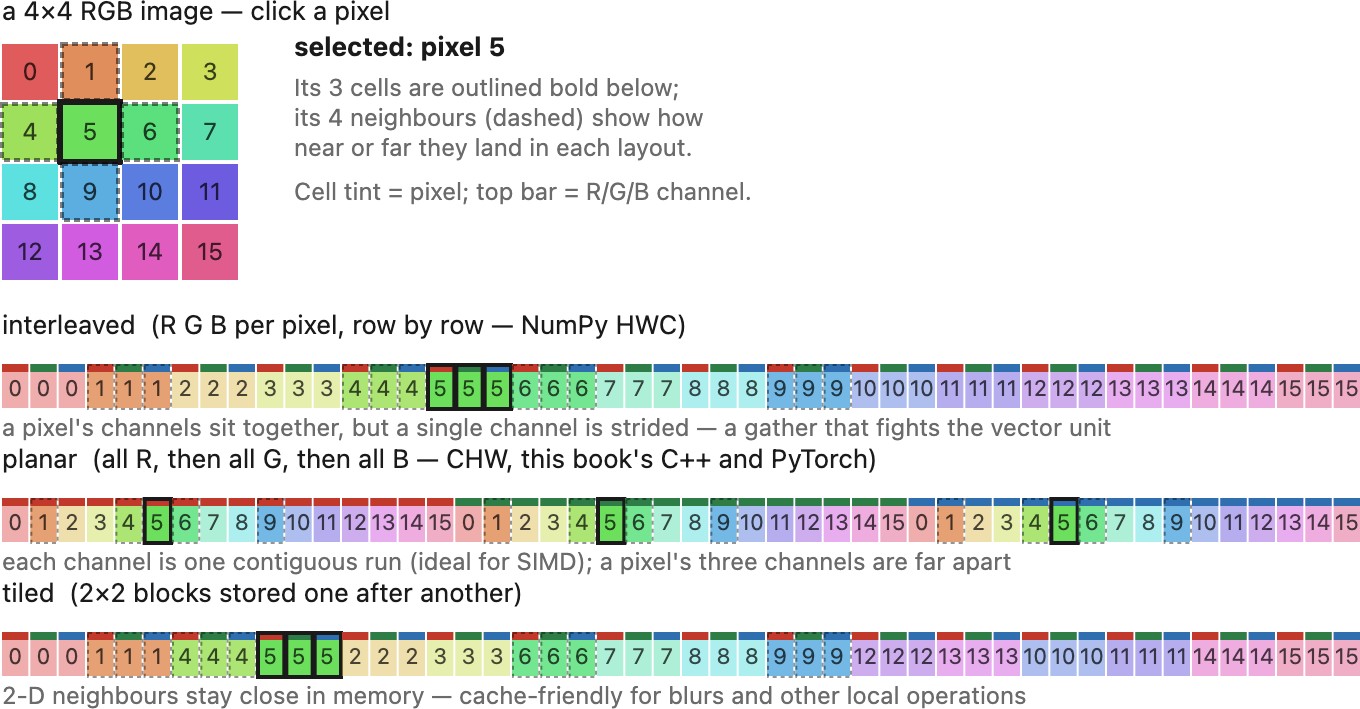
R G B together, row by row), planar (all the reds, then the greens, then the blues), and tiled (small 2×2 blocks laid one after another). To work on one channel, planar storage offers it as one contiguous run, the access a vector unit wants, while interleaving scatters it across every third cell. Tiled storage keeps a pixel's 2-D neighbors close together, which is what a local operation like a blur wants; no layout wins outright, you pick the one your access pattern rewards. Interactive: click a pixel to highlight its cells and its four neighbors across all three layouts, and flip the layout to watch the access pattern change.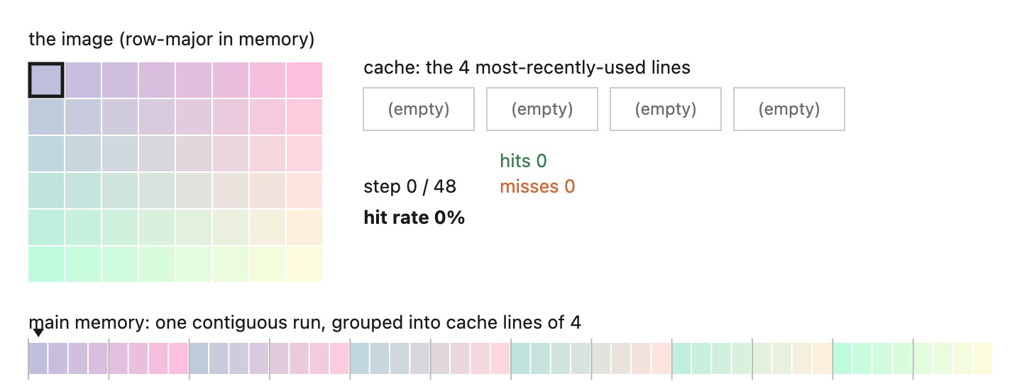
for y { for x } walks memory in order, so each miss loads a line that then serves the next several reads as hits; for x { for y } jumps a full row's stride every step, to a fresh line that is evicted before the loop returns, so almost every read misses. Same pixels, same arithmetic, very different hit rate. (A teaching model, real caches are larger and set-associative, but the locality effect is exactly this.) Interactive: play or single-step, and flip the loop order to watch the hit rate collapse.Prefer traversal that reuses nearby stored values. For scalar loops over packed HWC, use y, x, c order; for packed CHW, use c, y, x. Actual strides, tiling, and vectorized kernels can change the best schedule. Measure before changing the representation.
This book carries a concrete, working C++ image data structure; seeing it once makes the planar arithmetic above concrete. It is deliberately minimal: three integers for the shape, and a single flat buffer of floats in planar order:
struct Image {
    int width, height, channels;
    std::vector<float> data;        // planar: c*width*height + y*width + x

    Image(int w, int h, int c)
        : width(w), height(h), channels(c),
          data(static_cast<size_t>(w) * h * c, 0.0f) {}

    // The accessor: hides the index arithmetic, so the rest of the
    // code can think in plain (x, y, c).
    float& operator()(int x, int y, int c) {
        return data[static_cast<size_t>(c) * width * height + static_cast<size_t>(y) * width + x];
    }
};
This minimal accessor assumes validated nonnegative dimensions, a checked allocation-size product, and in-range indices. Use a sufficiently wide unsigned type for offset multiplication. A production image class also needs const access and explicit boundary reads; an unchecked mutable reference cannot implement zero padding safely. In Python, the book uses arr[y, x, c].
The accessor makes the storage choice concrete without spreading it through the rest of the program. A call such as img(x,y,0)=1.0f looks like indexing a three-dimensional image, while the function computes one offset into the flat buffer. Changing packing later requires changing this mapping and the code at library boundaries, rather than every mathematical expression. Read access beyond an image edge should be a separate policy from obtaining a mutable reference to a stored pixel.
The loop-order effect comes from reuse of fetched data. A cache line brings several neighboring values into the processor together. Traversing a packed row uses those values before moving on; jumping one full row per inner iteration can touch many cache lines while using only one value from each. A different schedule may recover that reuse through tiling or vectorization, which is why the benchmark measures the implemented loop rather than proving a universal ordering rule.
Developing, testing and debugging⧉
PS0 sets up the toolchain, a minimal image class, and image I/O. → Chapter 1.5, Problem sets.
A blur can return a valid image with a dark border. A resampler can produce a sharp picture full of aliasing. Neither needs to crash. Getting image code to work requires both checking its numbers and looking at what those numbers produce. Start with one stage and an input small enough to check by hand.
The workflow: build, run, look at the picture⧉
Save intermediate images and open them. This is the image-processing equivalent of a print statement. When the final image has black specks, inspect the inputs and outputs of the suspected stage, then check the values at those pixels. The first place a defect becomes visible helps localize the problem; an earlier numerical error may still be its cause.
A PNG is convenient for display, but a display copy is not the underlying array. Negative values, values above one, and small floating-point differences can disappear when you clip and quantize for export. Keep the original buffer or save a format that preserves its range and precision. Record its shape, type, color encoding, minimum, maximum, and counts of NaN and infinity. Chapter 8.1, Image representation explains why a buffer's interpretation matters as much as its values.
Use the same display transform and scale for comparisons. Independently normalizing two images can hide an incorrect gain. For signed differences, map zero to a neutral gray and positive and negative errors to opposite colors; state the amplification. Mark nonfinite values separately. A black difference image may mean agreement, or merely differences too small to survive the display conversion.
Write a helper that displays an array and reports its range. Make the scale explicit and easy to reuse. If inspecting an intermediate takes one line, you will do it while developing instead of only after the final output fails.
Test on inputs you can verify by hand⧉
optionalA tiny input lets you compare every output value against a calculation independent of the implementation. Use several sizes, including a non-square image, odd dimensions, and a single row or column. These expose transposed axes, vector tails, and boundary assumptions that a convenient square image misses.
- A constant tests the expected gain. A normalized blur with constant-preserving boundaries should return that constant; a derivative should return zero. Zero padding deliberately darkens the border of a nonzero constant, so decide whether that is the specified behavior before calling it a bug. For color code, use different constants in the three channels to expose channel swaps.
- An impulse tests how a local input spreads. For a linear, shift-invariant filter away from boundaries, the output gives the convolution kernel. For a general linear operator it gives one column of the operator, which may differ at another location. Test center and boundary impulses separately.
- A step edge exposes ringing, halos, shifts, and color fringes. Try both orientations and a diagonal.
- A rectangle adds corners and unequal extents. It is useful for checking coordinate conventions and differences between horizontal and vertical processing.
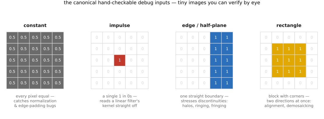
Apply these tests to individual stages. Compare integer results exactly when the specification requires it. For floating-point results, choose tolerances in the working units, accounting for rounding and changes in reduction order. One common comparison is
The absolute tolerance handles values near zero; the relative tolerance allows error proportional to magnitude. Check nonfinite values before this comparison. A large tolerance can conceal an algorithmic error, so report the maximum difference and its location as well as pass/fail.
A constant removes spatial variation. If a normalized blur changes its interior value, check the sum of weights and the arithmetic type. If only the border changes, check the extension rule. These are distinct failures with distinct fixes.
Apply the same discipline inside the pipeline: feed these inputs to your intermediate stages, not only to the final program. A failed whole-pipeline impulse test tells you that something is broken; running each stage on an impulse tells you which stage. The synthetic inputs and the binary-search habit are the same idea from two directions: small inputs make each stage checkable, and checking each stage localizes the bug.
Crashes and bounds⧉
optionalOut-of-bounds accesses are common in neighborhood operations: a neighbor at the left edge has a negative column, or the last row asks for a sample at height. In C++, an invalid read or write is undefined behavior. A write may corrupt adjacent memory and trigger a crash much later. Invalid reads, dangling pointers, and data races can also fail without a useful message.
Check indices at the point of access, use a debugger, and enable the compiler's memory-error diagnostics during development. Assert properties that the algorithm actually requires, such as valid extents or a nonzero normalization denominator. Do not assert that every intermediate lies in $[0,1]$: many linear filters and color transforms legitimately produce values outside that range.
Debug assertions help catch internal mistakes, but they do not replace input validation in a release build. Reject unsupported dimensions and formats at the interface. For intended accesses outside an image, apply the specified extension rule (repeat, mirror, wrap, or zero) before reading memory. An assertion catches an unhandled access; it does not choose the correct boundary condition.
Start with the first relevant diagnostic and reduce the code to a small example. Later errors may be consequences of the first. Documentation, a search, or an LLM can help interpret a message, but check that the proposed fix preserves the operation and types you intended.
Put a check where the assumption is first used. For example, a resampler can produce an invalid source coordinate long before an eventual crash in an unrelated allocation. Checking the coordinate immediately before the load identifies the operation that broke the contract. Similarly, after computing a normalized filter, check that its weights sum to the expected value; after a transform, check finiteness before sending the result to the next stage. The first failed invariant is usually more informative than the final wrong image.
Keep internal development assertions separate from input validation. A release build may disable assertions, but it still needs to reject unsupported external sizes, formats, and indices safely. Removing a debug check must not make malformed input legal.
C++ for Python programmers⧉
optionalThe problem sets in this book are written in C++, and if Python is your home language this appendix is the bridge. You are not expected to arrive knowing C++: the early psets ramp you up, and what follows is the map of what changes.
Why C++ at all? It is compiled and close to the metal, so the per-pixel loops that image processing lives on can run far faster than equivalent scalar Python loops; the gain depends on the workload and compiler, and is not a comparison with optimized NumPy kernels. It is still the standard where performance matters, in graphics and imaging, and it is the language Chapter 29.4, Halide programming plugs into for the last chapters. The price is bluntness: more typing, fewer guardrails, and memory you sometimes manage yourself. The good news is that for this book you stay in a small, safe corner of the language.
What changes, coming from Python⧉
optional- Compiled, not interpreted. You translate the whole program to machine code once, with the compiler, then run the resulting binary. A whole class of mistakes (a misspelled name, a type mismatch) is caught at compile time rather than when the line happens to run.
- Static types, declared up front. Every variable has a fixed type, written before its name:
int n = 5;,float x = 0.5f;. You cannot later rebindnto a string. Functions spell out the type of each argument and of the return value. - Semicolons and braces. Statements end in
;, and blocks are delimited by curly braces{ }, not by indentation. Indent for readability; the compiler ignores it. - Headers and implementation files in the course code. A header (
.h) declares what exists; an implementation (.cpp) defines it. You#includethe header, you do notimport. - Value semantics by default. Assigning or passing an object by value generally copies it, though moves and copy elision can avoid copies, unlike Python, where a name is a reference to a shared object. You ask for sharing explicitly, with a reference.
- A leaner toolkit. Fewer built-in higher-order conveniences; you write more loops by hand. These exercises do not use a C++ array library to do the work for you, so the loop over pixels is yours to write (and the compiler's to make fast).
- Memory is explicit, but mostly hidden here. There is no garbage collector, yet if you stick to local variables and
std::vectoryou almost never callnewordelete.
A first taste, side by side⧉
optionalBrighten an image by a constant factor, written as a function in each language. In Python the body is a single NumPy broadcast:
def brighten(im, factor):
    return im * factor
Assume floating-point NumPy inputs, with import numpy as np. In C++ with the course's Image class it is an explicit loop, and every difference above shows up at once:
Image brighten(const Image &im, float factor) {
    Image out(im.width(), im.height(), im.channels());
    for (int c = 0; c < im.channels(); c++)
        for (int y = 0; y < im.height(); y++)
            for (int x = 0; x < im.width(); x++)
                out(x, y, c) = im(x, y, c) * factor;
    return out;
}
Types on everything, the loop written out, const Image &im to pass the input by reference without copying it or letting the function change it, and semicolons throughout. The vectorization is gone, but the compiled loop is fast.
A few more comparisons⧉
optionalThe same algorithm three ways (the C++ clamp example needs C++17 and <algorithm>): plain Python with the explicit loops C++ makes you write, the C++ itself, and the vectorized NumPy one-liner. The shading marks what C++ adds over the plain-Python loops, only the static types, the punctuation, and std::; the loops themselves are identical. Switch tabs, and copy any of them:
def clamp01(im):
    out = np.empty_like(im)
    H, W, C = im.shape
    for c in range(C):
        for y in range(H):
            for x in range(W):
                out[y, x, c] = min(1.0, max(0.0, im[y, x, c]))
    return out
Image clamp01(const Image &;im) {
    Image out(im.width(), im.height(), im.channels());
    for (int c = 0; c <; im.channels(); c++)
      for (int y = 0; y <; im.height(); y++)
        for (int x = 0; x <; im.width(); x++)
          out(x, y, c) = std::clamp(im(x, y, c), 0.0f, 1.0f);
    return out;
}
def clamp01(im):
    return np.clip(im, 0.0, 1.0)
def luminance(im):
    H, W, C = im.shape
    out = np.empty((H, W, 1))
    for y in range(H):
        for x in range(W):
            out[y, x, 0] = (0.299 * im[y, x, 0]
                          + 0.587 * im[y, x, 1]
                          + 0.114 * im[y, x, 2])
    return out
Image luminance(const Image &;im) {
    Image out(im.width(), im.height(), 1);          // one output channel
    for (int y = 0; y <; im.height(); y++)
      for (int x = 0; x <; im.width(); x++)
        out(x, y, 0) = 0.299f * im(x, y, 0)
                     + 0.587f * im(x, y, 1)
                     + 0.114f * im(x, y, 2);
    return out;
}
def luminance(im):
    return (0.299 * im[:, :, 0:1] + 0.587 * im[:, :, 1:2]
            + 0.114 * im[:, :, 2:3])
def blend(a, b, t):
    out = np.empty_like(a)
    H, W, C = a.shape
    for c in range(C):
        for y in range(H):
            for x in range(W):
                out[y, x, c] = (1.0 - t) * a[y, x, c] + t * b[y, x, c]
    return out
Image blend(const Image &;a, const Image &;b, float t) {
    Image out(a.width(), a.height(), a.channels());
    for (int c = 0; c <; a.channels(); c++)
      for (int y = 0; y <; a.height(); y++)
        for (int x = 0; x <; a.width(); x++)
          out(x, y, c) = (1.0f - t) * a(x, y, c) + t * b(x, y, c);
    return out;
}
def blend(a, b, t):
    return (1.0 - t) * a + t * b
def mean(im):
    H, W, C = im.shape
    total = 0.0
    for c in range(C):
        for y in range(H):
            for x in range(W):
                total += im[y, x, c]
    return total / (H * W * C)
float mean(const Image &;im) {
    float total = 0.0f;
    for (int c = 0; c <; im.channels(); c++)
      for (int y = 0; y <; im.height(); y++)
        for (int x = 0; x <; im.width(); x++)
          total += im(x, y, c);
    return total / (im.width() * im.height() * im.channels());
}
def mean(im):
    return im.mean()
The luminance example retains the course's grayscale weights and function name: on encoded RGB these weights compute a luma-like quantity, not physical linear-light luminance. Inputs are nonempty; RGB examples need three channels, and blending requires matching shapes.
Across all of them the same shapes recur in the C++: const Image & for every input, im.width()/height()/channels() as the loop bounds, float literals with the f suffix, and a fresh Image out(...) to fill and return (or, for a reduction, a plain float). The plain-Python column makes the real point: the C++ loop is not exotic, it is the loop you would write in Python the moment you step off NumPy's vectorized path, with static types and braces bolted on. Once those are muscle memory the translation is mechanical, and making the loop fast is the compiler's job.
Files and compilation⧉
optionalA C++ project is split in two. The header Image.h declares the class and the function signatures; the implementation Image.cpp defines them. To use another module you #include "Image.h", which literally pastes its declarations in. Because a header can be included along several paths, each one is wrapped in an include guard, an #ifndef / #define / #endif sandwich that stops it being pasted twice; it looks archaic, and the template files already have it. A build tool (make, or CMake) reads a build file listing the sources and runs the compiler, so you compile the whole project with one command.
Two syntax traps trip people early. In a .cpp file the scope operator :: says which class a definition belongs to, as in float Image::operator()(int x, int y, int c), because one file can implement several classes. And a class definition needs a semicolon after its closing brace; forget it and the error surfaces, confusingly, in the next file.
Value, reference, and const⧉
optionalThis is the shift that trips Python programmers most, because Python hides it. How you declare a function's parameter decides whether it sees a copy or the original, and whether it may change it.
f(Image im)passes by value: an lvalue argument is copied into the parameter unless the class defines other behavior. Moving a temporary can avoid a copy.f(Image &im)passes by reference: the function works on the original, and changes it makes persist. No copy, so it is fast.f(Image *im)passes a pointer (a raw memory address). We avoid pointers in this book.f(const Image &im)passes by reference but read-only: fast, no copy, and the compiler forbids the function from modifying it. Thisconst &is how you pass most inputs.
A trailing const on a method, int width() const;, is the same promise from the other side: the method will not mutate the object, so getters are marked const and can be called on read-only inputs.
Memory, briefly⧉
optionalAn ordinary local object has automatic storage duration and is destroyed when its scope ends; its owned pixel buffer may live in dynamically allocated storage; Image im(w, h, c); is all you need, with no new. Heap allocation with new must be matched by delete, which is where leaks come from, so we lean on std::vector, which owns and frees its own storage. The one sharp edge to remember: array access is unchecked, so v[i] with i out of range does not raise an exception. It silently reads or corrupts unrelated memory, or crashes with a segmentation fault, often far from the actual mistake.
Images in C++⧉
optionalThe course wraps an image in a class holding a flat std::vector<float> (often normalized to [0, 1], but intermediate values can lie outside that range) together with its width, height, and channel count. A vector has a single index, so a 3-D image is packed into 1-D by strides. The book, like Halide, stores it plane by plane (all of one channel, then the next):
index of (x, y, c) = c * width * height + y * width + x
An accessor im(x, y, c) hides that arithmetic. It takes x first, unlike NumPy's usual [y, x, c] indexing, and keeps the code consistent with Halide later. The same layout and the reasoning behind it are in Chapter 8.1, Image representation.
Debugging, and the parts that hurt⧉
optionalThe recurring frustration of C++ is that errors surface far from their cause: the missing class semicolon breaks the next file, an out-of-bounds write crashes somewhere unrelated, a segmentation fault points at the symptom, not the bug. A few habits from the course make it bearable.
- Read compiler errors from the first one down; later ones are often fallout.
- Test each piece as you write it, on tiny inputs (a 3×3 image, a constant, a single edge) whose answer you can work out by hand. Do not write the whole thing and then run it.
- Print and save intermediates: write images to disk and look at them.
- On a segmentation fault, suspect an array index. Print the index and the size, or
assert(0 <= i && i < size). - Compiler errors and syntax are exactly what search and AI assistants handle well; use them, and acknowledge any AI help per the course policy.
Where to go next⧉
optionalThe first problem set (Chapter 45.3, Problem Set 0 — Environment and C++ basics) is a warm-up by design: set up the environment, compile the template, write a few lines with std::vector, and do a brightness or contrast point operation. The psets after it build the Image class, point and neighborhood operations, and onward. For a fuller Python-to-C++ walkthrough, the course points to Goldwasser and Letscher's Python to C++ guide and the cpp4py tutorial.
Recap: big lessons in this lecture
Prefer traversal that reuses nearby stored values. For scalar loops over packed HWC, use y, x, c order; for packed CHW, use c, y, x. Actual strides, tiling, and vectorized kernels can change the best schedule. Measure before changing the representation.