38.6 Active non-line-of-sight⧉
The corner camera taught us that a wall can be made to image what it hides, by reading a shadow. But a shadow is faint, one-dimensional, and silent about range. Suppose we are willing to bring our own light and our own clock. Then the wall becomes something stronger: a relay screen we can illuminate, watch, and time. Send a pulse of light at a visible patch of wall; the wall scatters it in all directions; some of it lands on an object hidden around the corner; the object scatters it again; some of that returns to the wall; and the wall scatters a third time back toward our detector. If we can measure how long each returning photon took, with timing resolution set by the spatial detail sought: a few picoseconds correspond to millimeters of optical path, then the travel time tells us the total path length, and the path length constrains where the hidden object must be. This is active non-line-of-sight imaging, one of the most striking uses of photographing light itself in flight (Velten et al. 2012).
38.6.1 Third-bounce geometry and time-of-flight⧉
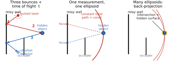
The thing to hold in your head is the three-bounce light path, because the entire method is the geometry of those three bounces plus a stopwatch. The light leaves the laser, hits a known spot on the wall (bounce one, whose timing we can calibrate away), travels to some unknown point on the hidden object (bounce two), and returns to a known spot on the wall that the detector is watching (bounce three). The detector measures the total time of flight of that round trip. Because the laser spot and the detector spot on the wall are both known, the only unknown in the path is the hidden point, and the measured time fixes the sum of the two unknown leg lengths, wall-to-object and object-to-wall.
A single time measurement does not locate the hidden point; it only says the point lies on an ellipsoid whose two foci are the illuminated wall spot and the watched wall spot (the locus of points for which the two-leg distance is constant). One measurement gives one ellipsoid, so the hidden object could be anywhere on it. But now move the laser spot to a different point on the wall, or watch a different spot, and you get a different ellipsoid. Each illuminated spot, paired with each detected return, contributes another ellipsoidal constraint. Where many ellipsoids intersect, the measurements support a candidate hidden surface, subject to noise and ambiguity. The reconstruction is therefore a back-projection: smear each measured return back onto its ellipsoid of possible origins, sum over all the wall spots you probed, and the hidden geometry lights up where the smears reinforce (Figure 38.6.1). It is tomography with light, where the projection geometry is set not by straight rays but by the constant-time-of-flight ellipsoids that pulsed light traces out.
38.6.2 The hardware: photographing light in flight⧉
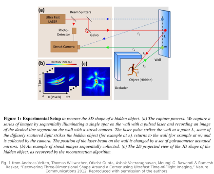
The reason active NLOS is hard, and the reason it belongs with Part 34, Computational sensors, is that fine spatial detail is encoded in very short time differences. A millimeter of path difference is about three picoseconds of light travel; tens of picoseconds correspond to centimeter-scale path differences, though spatial resolution also depends on relay-wall aperture, geometry, and reconstruction. Ordinary frame-rate imaging does not directly resolve these transients. The early demonstrations used a streak camera, the same instrument behind femto-photography in Chapter 34.10, Ultra High speed Imaging, which sweeps the arrival time of light across a spatial axis of the sensor, converting "when" into "where" and reaching roughly picosecond resolution along a line. Synchronize a streak camera to a femtosecond-pulsed laser and you can literally record a movie of the pulse propagating and returning; the NLOS reconstruction reads the hidden shape out of those time-resolved returns.
The streak camera is expensive, delicate, and slow to scan. The technology that made active NLOS practical is the single-photon avalanche diode (Chapter 34.5, Single-photon sensors (SPAD, avalanche, photon counting)): a detector that registers a single returning photon as a digital detection pulse that timing electronics can place in a fine time bin; detector jitter and the system impulse response limit actual temporal resolution. The third-bounce return is very weak because each scatter off a diffuse wall spreads the light over a hemisphere, and there are three such scatters, so the returning signal falls off catastrophically with distance and you are counting individual photons against a flood of directly-reflected ones. SPADs are built for exactly that regime: essentially zero read noise, photon-level sensitivity, and the timestamp the method needs. Modern systems pair a pulsed laser with a SPAD (or a small SPAD array), scan the laser over a grid of wall spots, and build a transient measurement, intensity versus time, at each, which is precisely the raw material the ellipsoidal back-projection consumes.
38.6.3 From back-projection to fast, exact inversion⧉
Naive back-projection works but is slow and blurry because every measurement contributes a full ellipsoidal smear, and you are summing millions of them. A line of work has since recast the inversion as a cleaner, faster operation. If you arrange the system confocally, illuminating and observing the same wall spot, scanning it together, after a change of variables and geometric weighting, an idealized three-bounce model becomes a convolution, and the reconstruction becomes a single deconvolution by a known kernel: the light-cone transform of O'Toole, Lindell and Wetzstein (O'Toole et al. 2018), which turns hours of back-projection into a fast, closed-form inversion and sharpens the result. Related reformulations borrow migration algorithms from seismic imaging, where geophysicists have been reconstructing subsurface structure from the timing of reflected waves for decades, and the reconstruction uses a closely related wave-back-propagation formulation, repurposed from sound in rock to light around a corner (Lindell et al. 2019). The lineage matters: the deeper idea, that you can recover what you cannot see by modeling and inverting how a probe wave scatters off it, is shared across radar, ultrasound, seismology, and now optical NLOS.
Before the ultrafast hardware existed, Kirmani and colleagues laid out the transient imaging framework that makes all of this principled: the idea that the time-resolved response of a scene to a light pulse contains, in its multiply-scattered later returns, information about geometry hidden from direct view (Kirmani et al. 2009). Active NLOS is the cashing-out of that framework once cameras fast enough to measure the transient arrived.
38.6.4 The trade, stated plainly⧉
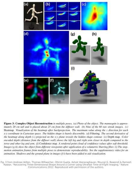
Active NLOS gives you a great deal: a real, depth-resolved, often two- or three-dimensional reconstruction of a hidden object's shape, robust enough to recognize letters, mannequins, and pose (Figure 38.6.3). That is far more than the corner camera's one-dimensional angular video.
The cost is substantial. You must supply a controlled, pulsed light source and aim it. You need sensitive detection and fast timing electronics. Many systems scan for seconds to minutes, fighting a signal so weak you are counting photons. And you generally need an unobstructed relay wall you can both illuminate and observe. Active NLOS spends hardware, light, and time to buy signal and depth.
The opposite bargain is the whole point of the next chapter. Chapter 38.7, Passive non-line-of-sight, throws away the laser and the picosecond clock, keeps only an ordinary camera and the ambient light that is already there, and asks how much of the hidden world you can recover from the faint, untimed structure that occluders leave in an ordinary photograph. Some passive methods recover a two-dimensional image from a snapshot; recovering depth needs additional constraints or measurements. The corner camera was the first taste of that passive route; the active route shows what controlled illumination and timing can add. Between them lies the real lesson of looking around corners: the wall is a relay, and what you can read off it depends entirely on whether you control the light that lands on it.