36.7 Photos → radiance fields and Gaussian splatting (NeRF, 3DGS)🔗⧉

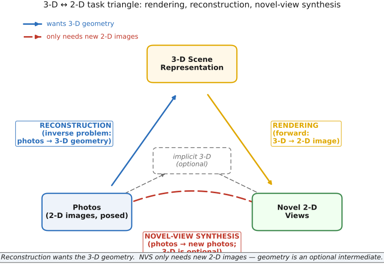
The classic pipeline of the previous chapter wanted geometry: a mesh, a point cloud, a thing you can measure or 3-D-print. But a huge and lucrative class of applications does not need the geometry at all, only new views of the scene. That is novel-view synthesis (NVS), and recognizing that it asks for less than reconstruction (new 2-D images, with 3-D only an optional intermediate) is what opened the modern era.

36.7.1 Two goals, one diagram🔗⧉

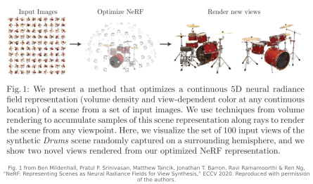
Three tasks live on one triangle (Figure 36.7.1⛶ fullscreen). Rendering goes 3-D → 2-D: given a scene, make an image (the forward direction, computer graphics). Reconstruction goes 2-D → 3-D: given photos, recover the scene geometry (the inverse direction, the previous chapter). Novel-view synthesis goes photos → new photos: given some views of a scene, produce others, and it may pass through a 3-D representation or it may not. The reason to separate NVS from reconstruction is that NVS is judged only by whether the new images look right, so it can use a 3-D representation that is excellent for re-rendering even if it would be a terrible mesh. That latitude is exactly what radiance fields exploit.

36.7.2 Inverse differentiable rendering, and the discontinuity that forced fuzziness🔗⧉

Here is the reframing that organizes everything. Suppose you have a scene representation with adjustable parameters $\theta$, and a renderer $R(\theta, \text{pose})$ that produces an image from any camera. If $R$ is differentiable in $\theta$, then fitting the scene to your photos is just optimization: minimize, over $\theta$, the difference between the rendered images and the captured photos,

by gradient descent. This is inverse, differentiable rendering, and it is a general recipe: whatever representation you choose, if you can render it differentiably, gradient-based optimization can attempt to fit it to images; nonconvexity and missing evidence still matter.

So why not fit a mesh of opaque triangles? Because the renderer is not smoothly differentiable in the geometry. A pixel's color is an integral over a discontinuous visibility function: at a silhouette edge, an infinitesimal move of a triangle flips a pixel from "object" to "background." Point-sampling that integral, as rasterizers and ray tracers do, misses the contribution of the moving silhouette entirely, so the naïve gradient with respect to geometry is zero where it should be informative, and spiky where the silhouette crosses a sample. Hard surfaces give sparse, unreliable gradients; gradient descent stalls.

The escape is to make the scene continuous and semi-transparent. If every point in space has a density and contributes a little to many pixels, then moving or recoloring it changes the rendered images smoothly, so the visibility integral becomes differentiable, gradients flow everywhere, and SGD works. This is an important motivation for volumetric and splat representations, alongside their ability to represent complicated appearance and topology. NeRF and Gaussian splatting are not fuzzy because the world is fuzzy; smooth opacity makes useful gradients easier to obtain. Hard-surface renderers can also be differentiated with estimators that handle visibility boundaries; differentiability is not exclusive to volumes. (It is also why they handle hair, foliage, and semi-transparency (the very things the hard-surface pipeline fails on) more flexibly, though fitting these effects still requires sufficient observations and an appropriate appearance model.)

36.7.3 NeRF: a scene as a tiny neural network🔗⧉

NeRF (Neural Radiance Fields Mildenhall et al. 2020) makes the representation an MLP (a small fully-connected network) that maps a 3-D position and a viewing direction to a color and a density:

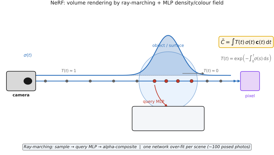
For samples $\mathbf x_i=\mathbf o+t_i\mathbf d$ on a unit-direction camera ray, the discrete rendering rule is

Here $\delta_i=t_{i+1}-t_i$ is the segment length, $\sigma_i$ its density, and $c_i$ its view-dependent color. The background receives the transmittance left after the final sample. Density is not itself opacity: the conversion depends on segment length. Finer sampling should approximate the same integral, rather than make the volume arbitrarily more opaque.

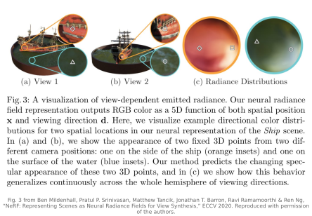
The original architecture makes density depend on position, not viewing direction; direction conditions color. To render a pixel, march a ray out from the camera, sample many points along it, query the MLP at each, and alpha-composite the samples front-to-back, weighting each by its density and by how much light survives to reach it, the classic volume-rendering integral (Figure 36.7.4⛶ fullscreen). Because density and color are continuous functions of position, the sampled volume-rendering computation supports gradients, and the network is overfit to one scene from on the order of a hundred posed photographs: it does not generalize across scenes, it is a compressed representation of this one scene that happens to be stored in network weights. Making color depend on view direction lets it reproduce view-dependent effects, such as specular highlights that move as you orbit, exactly the thing view-dependent texture mapping chased. The results are photorealistic and compact (a few megabytes of weights for a whole scene). The costs are speed: ray-marching queries the MLP hundreds of times per pixel and wastes most of that effort in empty space, making both training and rendering slow.

36.7.4 Do we even need the network?🔗⧉

Two follow-ups showed that most of what makes NeRF work is the differentiable volumetric optimization, not the neural network. Instant-NGP Müller et al. 2022 kept a small MLP but stored features in a multiresolution hash grid, reducing scene-fitting time dramatically, to seconds for demonstrated settings; rendering speed also improves, with costs depending on scene, hardware, and quality; the lookup, not the network, does most of the work. Plenoxels Fridovich-Keil, Yu et al. 2022 (Plenoxels) went further and removed the network entirely: a sparse voxel grid storing density and spherical-harmonic color directly, optimized by the same inverse-rendering loss, matches NeRF quality with no neural network at all. These results separate the value of differentiable volumetric fitting from the choice of an MLP parameterization. The MLP was one convenient parameterization of the field; a grid works as well or better.

36.7.5 3-D Gaussian splatting: the lessons without the deep learning🔗⧉

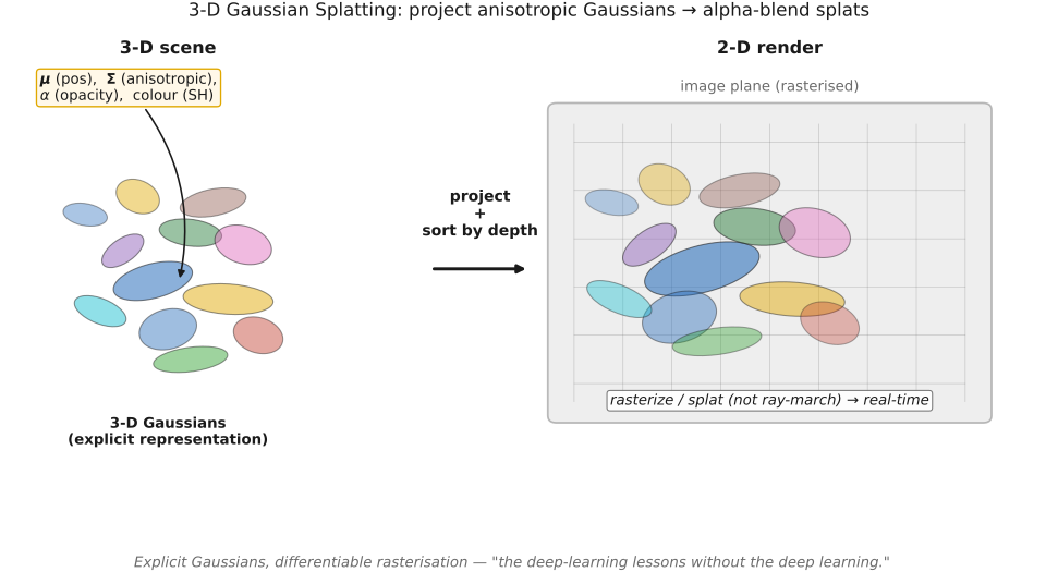
3-D Gaussian Splatting (3DGS) Kerbl et al. 2023 takes that lesson to its conclusion and reaches real-time rendering at high quality. The scene is represented as millions of explicit 3-D Gaussians, each a little fuzzy ellipsoid with a mean (position), a covariance (anisotropic size and orientation), an opacity, and a view-dependent color stored as spherical-harmonic coefficients (Figure 36.7.5⛶ fullscreen). Rendering does not ray-march: it rasterizes, projecting ("splatting") each 3-D Gaussian to a 2-D ellipse on the image plane, sorting them by depth, and alpha-blending front-to-back. Because rasterization is fast and the Gaussians are explicit, rendering is real-time, and the splat weights supply useful derivatives, although sorting, culling, and densification introduce discrete decisions, so the Gaussians' positions, shapes, opacities, and colors are all optimized against the photos (with adaptive densification that adds Gaussians where detail is missing and pruning that removes near-transparent ones). It carries the deep-learning lessons without any deep learning: no network, just an explicit, differentiable, volumetric point cloud, the Plenoxels idea made anisotropic, sparse, and real-time.

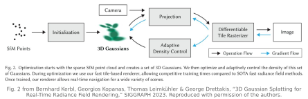
These results do not translate well to still figures, because the main point is smooth, free-viewpoint motion through a reconstructed scene, so they are best watched. The authors' own result videos, in chronological order, show the three-step arc (slow MLP → instant grid → real-time splats) clearly:

36.7.6 The practical recipe: and what is baked in🔗⧉

Here is what a reader can actually do. Capture tens to hundreds of overlapping photos of a static scene, orbiting to cover it. Run COLMAP SfM (the front end from the previous chapter) to recover the camera poses and a sparse point cloud that seeds the Gaussians (or initializes the radiance field). Optimize the representation against the photos (minutes for a splat, longer for a vanilla NeRF) with densify/prune along the way. Then drop the result into a real-time viewer and fly around (Figure 36.7.7⛶ fullscreen). This is the dense-optimization end of a spectrum whose other end is the light fields / unstructured lumigraph of Chapter 31.1, Light fields 101 and Chapter 31.7, Lumigraph and shape priors for sharper light field rendering: sample the rays directly (light fields) versus fit a model to the rays (radiance fields) are two answers to the same NVS question Levoy & Hanrahan 1996 Gortler et al. 1996 Buehler et al. 2001.

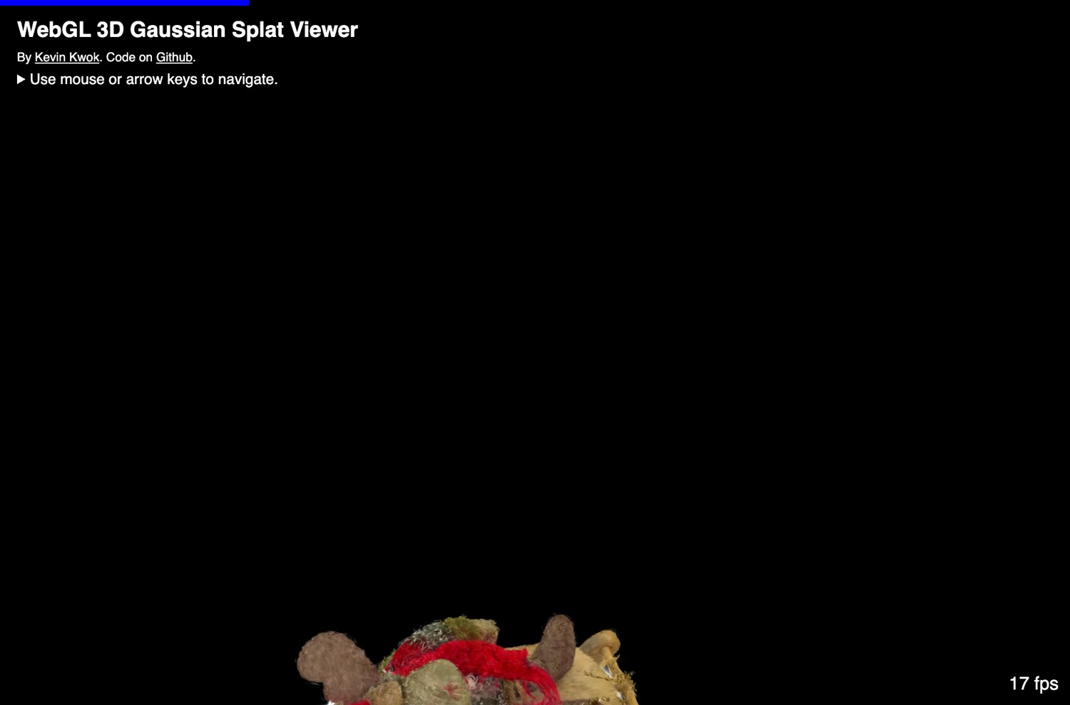
State plainly what is baked in, because it is the source of most disappointment. The illumination is fixed: view-dependent color is not a relightable material model (BRDF), so you cannot change the lighting of a captured splat, only the viewpoint. It is one scene per model: nothing transfers to the next scene; you optimize again from scratch (the pain point the next chapter attacks). And quality is bounded by capture coverage: regions the photos under-saw produce "floaters" and smeary artifacts, because the optimization had no photo to constrain them. Within those limits, fixed lighting, one scene, and good coverage, the result is a real-time, photorealistic, free-viewpoint scene from nothing but a phone's worth of photos.

36.7.7 Relaxing the assumptions: NeRF in the wild🔗⧉

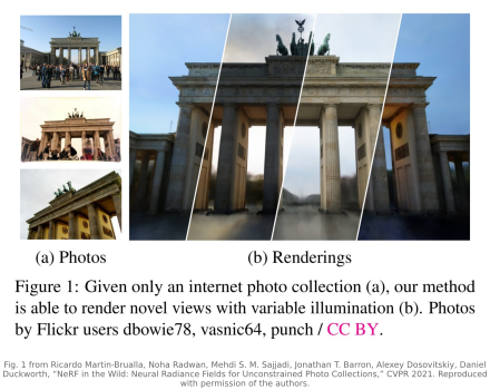
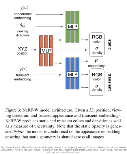
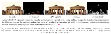
Two of those baked-in assumptions, a controlled capture and fixed lighting, are exactly what NeRF in the Wild (NeRF-W) Martin-Brualla et al. 2021 (NeRF in the Wild) sets out to relax, by fitting a radiance field to uncontrolled internet photo collections: the thousands of tourist snapshots of a landmark that already exist, shot on different cameras across years, weather, and times of day, and cluttered with people and cars that come and go. A vanilla NeRF, which assumes every photo sees the same static scene under the same light, collapses on such data. NeRF-W's fix is to hand the network two per-image latent embeddings, learned jointly with the field: an appearance embedding that absorbs the lighting, exposure, and white-balance differences between photos, and a transient embedding feeding a second, transient MLP (plus a learned uncertainty field) that explains and then discounts the movable clutter, so the static reconstruction can reduce their influence; imperfect separation can leave artifacts. The static density is produced before the network sees the appearance embedding, which forces the geometry to stay shared across all images while each photo keeps its own look, so you can re-render the landmark with learned appearance codes. These codes do not supply a calibrated, physically relightable illumination/material decomposition. It is the direct answer to this chapter's "fixed lighting, controlled capture" limits, and it also belongs to the internet-photo-collection lineage of Chapter 28.5, Photo tourism.