36.1 Multiple view geometry🔗⧉

A single photograph is missing one number per pixel: the depth $Z$. The perspective projection $x = fX/Z$, $y = fY/Z$ of Chapter 2.2, Pinhole Image Formation and linear perspective maps a whole ray of 3D points (every point in the same direction but at a different distance) onto one image point, and the division by $Z$ that shrinks distant objects also erases how distant they were. You can recover $Z$ with extra hardware (the structured-light and time-of-flight depth sensors mentioned earlier), but the oldest and most general way to get it back is simply to look from a second place. That is what your two eyes do, what a stereo rig does, and what a moving camera does over time; the geometry is the same in every case, and this chapter is about that geometry.

First the intuition, which is genuinely simple and which evolution discovered long before we did: a nearby object shifts more than a far one when you change viewpoint, and that shift, the disparity, maps directly to distance. Then a teaser of the algebra that makes two-view geometry into a precise tool: the fact that a point in one image constrains its match in the other to a line, not a point, and the single small matrix that encodes that constraint. The intuition we develop in full; the algebra we state and forward to the multi-view chapters later in this part, where the multi-view machinery (many cameras, structure from motion, neural scene representations) properly belongs.

36.1.1 Two views: stereo and disparity🔗⧉

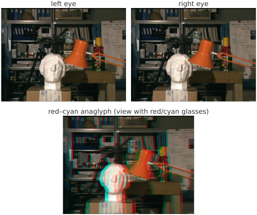
One camera throws away depth. Two cameras, looking at the same scene from slightly different positions, can get it back, which is why you have two eyes (Figure 36.1.1⛶ fullscreen). The cue is disparity: a nearby object shifts a lot between the two viewpoints, a faraway object barely shifts at all. Hold a finger close and blink each eye in turn and it jumps; do the same with a distant building and it stays put. That difference in shift is depth information, and your visual system fuses the two retinal images into a single sense of three dimensions, called stereopsis.

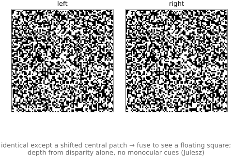
That disparity alone carries depth, with no help from recognizing objects or monocular cues like shading, occlusion, or familiar size, is not obvious. Bela Julesz proved it with the random-dot stereogram (Figure 36.1.2⛶ fullscreen). Take a field of random black-and-white dots, copy it for the second eye, and shift a central square patch sideways. Each image on its own is pure noise, with nothing recognizable in it. But fuse the two and a square floats crisply in front of the background. "Depth without objects": the visual system computes depth purely from the per-pixel shift, before it has any idea what it is looking at. This demonstrates stereopsis without recognizable monocular objects, and it is the conceptual ancestor of every stereo-matching algorithm.

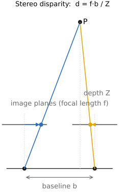
The geometry, for parallel cameras. Put two cameras side by side, optical axes parallel, separated by a baseline $B$, both with focal length $f$. A scene point at depth $Z$ projects into each camera; because the cameras are displaced by $B$, its two image positions differ by the disparity $d$. Drawing the two projection triangles and using similar triangles, the same move as in the perspective equation of Chapter 2.2, Pinhole Image Formation and linear perspective, gives the relation:

Read it back: depth is focal length times baseline, divided by disparity. A larger shift $d$ means a closer point (small $Z$); a vanishing shift means a far point ($Z \to \infty$). This is the finger-versus-building intuition, now written quantitatively. A wider baseline $B$ or a longer focal length $f$ spreads the disparities out and measures depth more precisely, which is why stereo rigs, and our two eyes, have a baseline at all (Figure 36.1.3⛶ fullscreen). The same relation also explains stereo's main limitation: because $d \propto 1/Z$, faraway points crowd into tiny, nearly equal disparities, so depth precision degrades with distance: for a small disparity error $\sigma_d$, depth uncertainty scales approximately as $\sigma_Z \approx Z^2\sigma_d/(fB)$. Increasing baseline improves this sensitivity but can reduce shared visibility and make matching harder.

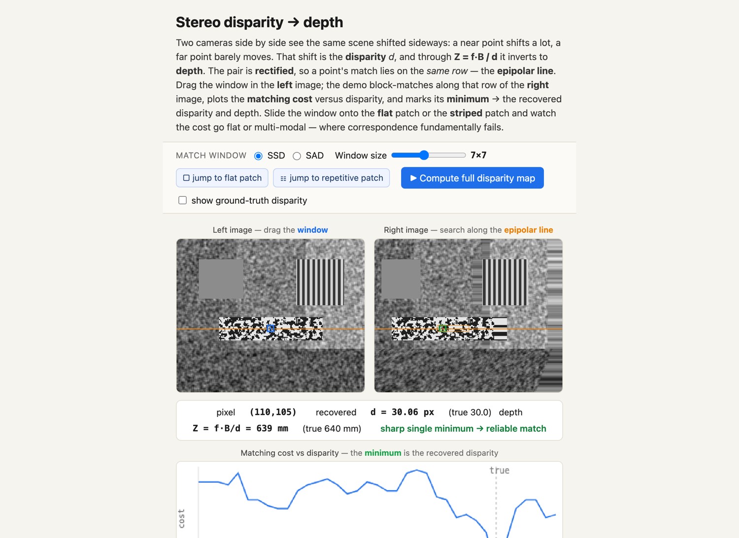
Stereo matching, finding each point's match in the other view and reading off its disparity, produces a disparity map, and through $Z = fB/d$, a depth map (Figure 36.1.4⛶ fullscreen). Real rigs are rarely perfectly parallel, so a preliminary step rectifies the pair: a separate homography for each undistorted pinhole image reprojects the pair as if the cameras were parallel, after which matching need only search along horizontal lines. That same homography machinery stitches panoramas (images taken from one viewpoint in different directions are also related by a homography) and the dual-pixel autofocus of a modern camera (covered in Chapter 5.3, Viewpoint, lenses, and focus) is a stereo pair the width of a single lens. The hard part of matching is always the same: textureless regions and occlusions, where a point has no distinctive match or no match at all. The full multi-view story (many cameras, structure from motion, neural radiance fields, and Gaussian splatting) is the subject of the multi-view chapters later in this part. Here the point is just the lever: two views plus disparity equals depth.

36.1.2 Two-view geometry: epipolar lines, and the essential and fundamental matrices🔗⧉

The parallel-camera picture is the easy case, where matches lie on the same horizontal row. The general two-view setup, two cameras in arbitrary positions and orientations, has a deeper structure that rests on a single fact we should see once even though we defer its algebra. The fact is this: a point in one view constrains its match in the other image to a whole line.

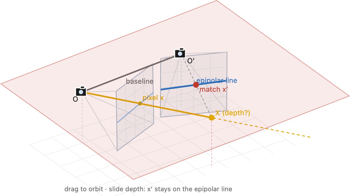
Here is why, in one picture (Figure 36.1.6⛶ fullscreen). Take a pixel in the left image. By the divide-by-$Z$ logic of projection, you do not know its depth, so its 3D point could be anywhere along a single ray shooting out from the left camera's center through that pixel. Now look at that whole ray from the right camera: the ray is a line in space, and a line in space projects to a line in the right image. So the match for your left pixel, wherever it turns out to be, must lie somewhere on that projected line, the epipolar line. Matching therefore reduces to a 1-D search along the epipolar line. This is a major simplification and the reason we rectify stereo pairs: rectification reprojects both images so that every epipolar line becomes a horizontal row, recovering the easy parallel-camera case of the previous section.

That point-to-line constraint is encoded by a single $3 \times 3$ matrix, and we can derive it directly from the picture just drawn, in the order ray, plane, then line.

Step 1: the ray (depth ambiguity). Work in the first camera's frame, with its center at the origin. A pixel back-projects to a ray: in calibrated coordinates (the pixel $x$ premultiplied by the inverse intrinsics, $\hat{x} = K^{-1}x$, which strips out focal length and principal point and leaves a pure direction) the unknown 3-D point is

where with the last coordinate of $\hat{x}$ normalized to one, $\lambda$ is axial depth, the quantity the divide-by-$Z$ projection threw away. The true point could sit at any $\lambda$ along this ray.

Step 2: the epipolar plane. That ray, together with the second camera's center, spans a plane: the epipolar plane. Equivalently, it is the plane through the two camera centers and the unknown point $X$. Whatever $\lambda$ turns out to be, $X$ lies in this one plane (Figure 36.1.6⛶ fullscreen).

Step 3: the epipolar line. The plane cuts the second image in a line, the epipolar line, so the match $\hat{x}'$ must lie on it. That is steps 1–3 of the picture; now we just write the plane down.

Step 4: the plane equation, in the second camera's frame. Let the second camera be rotated and translated from the first by $(R, t)$, so a point with first-frame coordinates $X$ has second-frame coordinates $R X + t$. Two facts follow:

• the first camera's center, the origin of frame 1, maps to $t$, so $t$ is the baseline vector from the second center to the first;
• the ray direction $\hat{x}$ becomes $R\hat{x}$ in the second frame.

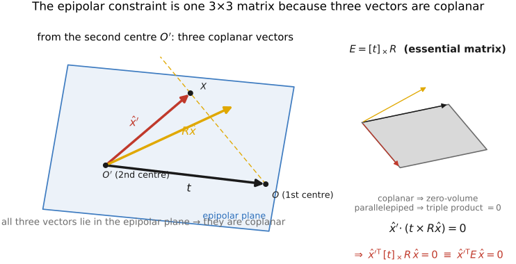
Now collect the three vectors that emanate from the second center into the epipolar plane: the match direction $\hat{x}'$ (toward $X$), the baseline $t$ (toward the first center), and the rotated ray $R\hat{x}$ (along the ray itself). All three lie in that one plane, so they are coplanar (Figure 36.1.7⛶ fullscreen). Coplanarity of three vectors is exactly a vanishing scalar triple product:

Writing the cross product $t\times(\cdot)$ as the skew-symmetric matrix $[t]_\times$ turns the triple product into a bilinear form, and that is the matrix:

$E = [t]_\times R$ is the essential matrix: the entire epipolar constraint in calibrated coordinates, assembled from nothing but the relative pose $(R, t)$.

From $E$ to $F$. In raw pixel coordinates the intrinsics are unknown or unremoved; with $x = K\hat{x}$ and $x' = K'\hat{x}'$ for the two cameras' intrinsics $K, K'$, substitute $\hat{x} = K^{-1}x$ and $\hat{x}' = K'^{-1}x'$:

This is the fundamental matrix $F$: the same constraint when the cameras are uncalibrated. It also closes the loop with the picture: $F x$ is a 3-vector of line coefficients, the epipolar line in the second image, so $x'^{\mathsf{T}}(F x) = 0$ says precisely "the match $x'$ lies on that line."

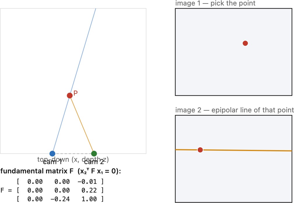
You can drive the whole construction yourself (Figure 36.1.8⛶ fullscreen): pick a point in the first image, slide its depth to move the 3-D point along its back-projection ray, and watch the point's image in the second view slide along the epipolar line (never off it) while $F$ is recomputed live from the two cameras' pose. Move the second camera (baseline and toe-in) and the whole epipolar geometry, and the epipole, shift with it.

What this buys, and what we still defer. Everything in two-view geometry flows from this one matrix. Because $E = [t]_\times R$, the relative pose $(R, t)$ of the two cameras can be recovered from $E$ (the translation only up to scale, because a single pair of images cannot know the absolute size of the world), with several pose candidates disambiguated by requiring triangulated points to lie in front of both cameras. Multiple views then require a consistent reconstruction and bundle adjustment, rather than merely chaining independently scaled translations. Pure camera rotation gives no triangulation baseline, and planar scenes create important estimation degeneracies. What we still leave to the multi-view chapters later in this part is the estimation and the scaling-up: recovering $F$ or $E$ from noisy point matches (the eight-point algorithm and its robust, RANSAC-wrapped descendants), the rectification math, triangulation (intersecting two verified rays to recover the 3-D point), and the leap to many images, including structure from motion and multi-view stereo, and the neural scene representations built on top of them. Keep the small, durable core: a second viewpoint gives depth; disparity inverts to distance through $Z = fB/d$; and in general a point constrains its match to an epipolar line: $x'^{\mathsf{T}} F x = 0$, with $F = K'^{-\mathsf{T}}[t]_\times R\,K^{-1}$ and its calibrated heart the essential matrix $E = [t]_\times R$.