34.7 Event sensors🔗⧉

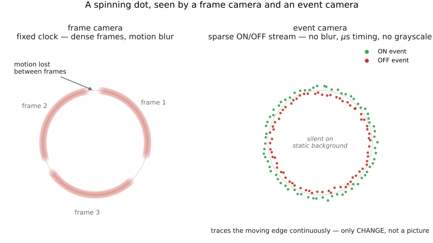
Almost every camera in this book is a clock-driven machine: on each tick of a shared shutter, every pixel reports its brightness, and the result is a frame. This is wasteful. Most of the scene usually isn't changing, so the sensor spends most of its data, power, and time re-transmitting a world that already sat still in the last frame, and anything that did move during the exposure is smeared into motion blur. The event sensor (or dynamic-vision sensor, DVS) throws the clock away. Each pixel runs independently and stays silent until the light it sees changes by a set amount; the instant it does, that one pixel fires a timestamped message, brighter here, now or darker here, now, and nothing else. A static scene produces near-silence; a moving edge sprays out a sparse stream of events with microsecond timing. There is no global frame exposure in a pure event stream, though the pixel circuit has finite bandwidth and response time. The sensor reports change, not state.

This inversion, asynchronous and differential rather than synchronous and absolute, defines the sensor. It buys a long list of advantages and exacts an equally structural price, and it forces nearly the entire downstream toolkit, built for dense synchronous arrays, to be rethought.

34.7.1 How it works: per-pixel change detection🔗⧉

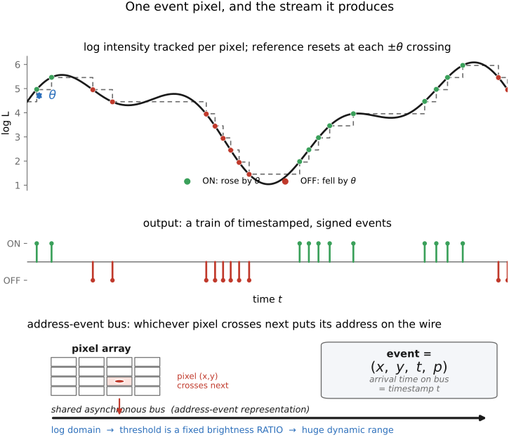
Each pixel of an event sensor continuously monitors the logarithm of the light falling on it. Working in log is the key design choice: a fixed log step is a fixed ratio of brightness, so the same threshold means "20% brighter" whether the pixel sits in deep shadow or bright sun, which gives the ratio-based sensitivity the eye has and the reason these sensors handle enormous dynamic range. The pixel remembers the log-intensity at which it last spoke. The moment the current log-intensity has risen by a threshold $\theta$ above that memory, the pixel emits an ON event (got brighter) and resets its memory to the new level; if it falls by $\theta$, it emits an OFF event (got darker). Each event is thus a tuple, pixel address, timestamp, polarity, and the pixel immediately re-arms to catch the next threshold crossing.

Because pixels fire independently and whenever they like, their events are read off the chip by an address-event representation (AER): a shared asynchronous bus over which each pixel announces its $(x, y)$ address and polarity the moment it fires, the time of arrival serving as the event's timestamp (Figure 34.7.1⛶ fullscreen). There is no row-by-row scan, so there is no rolling shutter and no global frame time, just a single time-ordered stream of events from across the array, each marking one threshold crossing at one pixel at a timestamp resolution set by the device. Bus contention and circuit latency can delay or perturb that timestamp.

34.7.2 The upside: microseconds, dynamic range, no blur, little data🔗⧉

The differential, asynchronous design wins on several axes at once, and they all trace to the same root.

• Microsecond temporal resolution. A pixel reports a change with microsecond-scale timing under favorable illumination and contrast, independent of any frame rate. Effectively the sensor "samples" at the equivalent of hundreds of thousands of frames per second, but only where and when something is actually changing.
• No motion blur. Blur comes from integrating a moving scene over an exposure window. An event pixel has no exposure window; it marks the instant an edge passes, so moving edges can be localized much more sharply in time. Finite photoreceptor bandwidth, especially in low light, and event-readout congestion still cause latency and missed changes.
• Very high dynamic range. Logarithmic response permits a wide operating range, often around 120 dB for specified devices and conditions. It does not give equal sensitivity or latency in starlight and sunlight: noise, leakage, contrast threshold, and bandwidth remain illumination-dependent. Comparisons with frame sensors need a common measurement criterion.
• Low data and low power. A still part of the scene generates few signal events, though dark activity and static bias power remain; the data rate depends on scene activity as well as array size and thresholds. Camera motion or flicker can activate much of the array and exhaust its bandwidth. An always-on event sensor can watch for motion at milliwatts, which is why they appear in battery-bound eye-tracking and surveillance.

34.7.3 The downside: no picture, and a new kind of data🔗⧉

Each advantage comes with a real cost. An event sensor does not produce an image. Its pixels report change in log-brightness, so a static image under constant illumination produces no ideal signal events, and there is no absolute intensity anywhere in its output; you cannot point it at a painting and get a photograph. This is why event cameras are frequently paired with a conventional sensor (or with a hybrid pixel that emits both events and occasional absolute frames, like the DAVIS sensor): the events supply the timing and the frames supply the appearance.

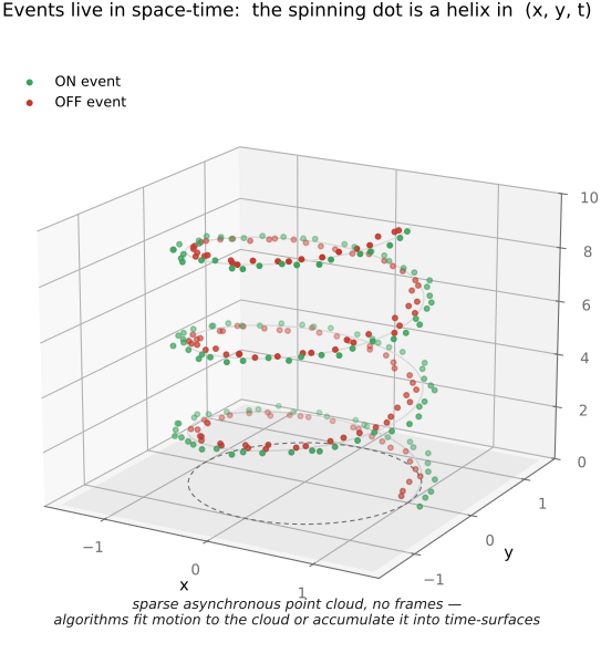
The deeper cost is to algorithms. The entire computer-vision and image-processing toolkit assumes a dense, synchronous array of intensities, with convolutions over a grid, frame differences, features computed on a picture. An event stream is none of those: it is a sparse, asynchronous point cloud in space-time, $(x, y, t, \text{polarity})$, with no frames to convolve and no fixed sampling rate. Working with it requires different machinery, such as accumulating events into time-surfaces or voxel grids, processing them event-by-event with recurrent or spiking networks, or fitting motion directly to the space-time event cloud, an active research area surveyed by Gallego et al. 2022.

34.7.4 Uses, lineage, and the contrast with single-photon🔗⧉

This trade-off, strong on change detection and weak for static appearance, makes event sensors useful for the tasks frame cameras handle worst. High-speed tracking and robotics: catching a thrown ball or a fast gesture with microsecond latency rather than waiting a frame. Visual odometry and SLAM: estimating a drone's or car's motion robustly through fast movement and harsh lighting where a frame camera would blur or clip. Deblurring and high-speed reconstruction: the event stream constrains brightness changes during a long-exposure frame, so the two together can reconstruct a sharp, high-frame-rate video. Augmented reality and eye tracking: low-latency, low-power, always-on sensing of where a fast-moving eye or hand is, where a frame sensor's power and latency are prohibitive. These are usually done with the event camera alongside a conventional one: events for when and where it moved, frames for what it looks like.

The lineage runs back to neuromorphic engineering, Carver Mead's program of building circuits that compute the way nervous systems do, and the event pixel is a direct descendant of Mahowald and Mead's silicon retina, mimicking how the retina's ganglion cells fire on changes in light rather than reporting a steady image. The first practical imaging DVS was Lichtsteiner, Posch and Delbrück's 128×128 sensor in 2008 Lichtsteiner et al. 2008; they are now sold by iniVation and Prophesee, the latter in a high-definition stacked sensor co-developed with Sony.

Chapter 34.5, Single-photon sensors (SPAD, avalanche, photon counting) and the event sensor are siblings: both can produce discrete detections that require different processing. Timestamping SPADs are asynchronous, while counting SPAD arrays and QIS can also output synchronous frames. But they report different events. A SPAD fires on the arrival of a single photon; it measures light, at the ultimate sensitivity, and timestamps it for ranging. An event pixel fires on a change in brightness; it measures temporal contrast, which can come from motion or illumination change. One is the sensor for the darkest scene; the other is the sensor for the fastest one. Together with the velocity pixel of Chapter 34.6, Doppler / velocity imaging, they complete this part's argument: that the richest cameras are built by deciding, per pixel, to measure the specific quantity an ordinary frame does not measure: a photon's arrival, a surface's velocity, or a brightness change, and then rebuilding the algorithms to match.