34.4 Depth sensors⧉
A camera throws depth away. Perspective projection maps a world point $(X, Y, Z)$ to an image point by dividing by $Z$ ($x = f\,X/Z$, $y = f\,Y/Z$; see Chapter 2.2, Pinhole Image Formation and linear perspective), and in doing so it collapses the depth axis: every point along a ray lands on the same pixel, and $Z$ is gone. Recovering that lost $Z$, per pixel, is one of the oldest and most consequential problems in imaging, and there is no single right answer, only several physical strategies, each emitting (or not) some signal and timing or triangulating its return. This chapter lays out that menu. The organizing question for every entry is: what does it send into the scene, and what does it measure coming back?
A first cut splits the field in two. Passive methods emit nothing and work from ordinary light. They are cheap and unobtrusive, but defeated by scenes that do not cooperate. Active methods project their own light, such as a pattern or a timed pulse, buying robustness on blank or dark surfaces at the cost of power, an emitter, and trouble in bright sun. We walk from passive to active, then close on the timing-based methods (LiDAR and time-of-flight) that increasingly dominate.
34.4.1 Stereo: passive triangulation⧉
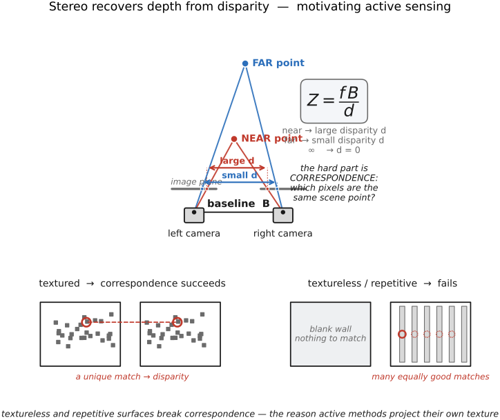
The reference design, and the one biology chose twice (our two eyes), is stereo: two cameras a fixed baseline $B$ apart. A world point projects to slightly different image positions in the two views, and the horizontal difference between them, the disparity $d$, depends only on depth. For rectified, parallel cameras the relation is exact and simple:
Near things shift a lot between the eyes (large disparity), far things barely shift (small disparity), and points at infinity have zero disparity, the same geometry that lets you gauge distance by alternately closing each eye. Measure $d$ at every pixel and the divide-by-$Z$ is undone.
The entire difficulty hides in measuring $d$: you must decide, for each pixel in the left image, which pixel in the right image is the same scene point: the correspondence problem. On rich, textured surfaces this is tractable (match a patch along the epipolar line, the subject of Chapter 36.1, Multiple view geometry), and Julesz's random-dot stereograms proved the brain solves it from pure disparity with no recognizable features Julesz 1971; the Middlebury benchmark drove decades of stereo algorithms Scharstein & Szeliski 2002. But correspondence fails exactly where the scene has nothing to match: a blank white wall (no texture to anchor a match), a repetitive pattern like a brick wall or a picket fence (many equally good matches, the aperture or ambiguity problem), a specular highlight that moves between views, or an occlusion visible to only one camera. That failure mode is the whole motivation for going active.
34.4.2 Structured light: projecting the texture⧉
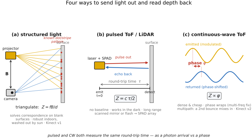
If a blank wall defeats stereo because it has no texture, put texture on it. Structured-light sensors replace one of the two cameras with a projector that casts a known pattern, such as parallel stripes, a grid, phase-shifted sinusoids, or a pseudo-random speckle pattern, onto the scene. Because the projected pattern is known, the system knows what it is looking for, so correspondence can be constrained even on a surface without natural texture: find where each projected feature landed and triangulate, one camera plus one projector, using calibrated camera-projector triangulation, reducing to $Z=fB/d$ in rectified coordinates with the projector playing the second viewpoint Geng 2011 (structured light).
The famous consumer example is the original Kinect (v1), 2010: a near-infrared laser projected a fixed PrimeSense speckle pattern of thousands of dots, and an offset IR camera recovered dense depth in real time by matching the observed dot field against a reference Smíšek et al. 2013, cheap enough to put real-time depth in living rooms and spark a wave of depth research (it is the front end of the real-time 3-D reconstruction of Chapter 36.1, Multiple view geometry Newcombe et al. 2011 (KinectFusion)). Industrial 3-D scanners instead sweep phase-shifted sinusoidal stripes (phase-shift profilometry) for sub-millimeter accuracy. Structured light works well indoors and at short range, producing dense depth, which is why it powers face-unlock dot projectors on phones, but the projected pattern is easily washed out by bright sunlight, struggles on specular or very dark surfaces that don't return the pattern cleanly, and has limited range (the pattern dims with distance). For the open road and longer ranges, you stop triangulating and start timing light.
34.4.3 LiDAR and direct time-of-flight⧉
The most direct way to measure distance is to time how long light takes to come back. Emit a brief laser pulse and measure the round-trip time $\tau$ to its echo; since light travels at $c$, the range is
(the factor of two for the round trip). Here $R$ is distance along the viewing ray, not axial depth $Z$; at viewing angle $\theta$ from the optical axis, $Z=R\cos\theta$. This is direct (pulsed) time-of-flight, and a system built on it is a LiDAR (light detection and ranging). Unlike triangulation, it needs no baseline and no correspondence; each direction's range comes from its own echo, so it avoids stereo's quadratic sensitivity of depth to disparity error. Return strength, timing uncertainty, and atmospheric or target effects still make ranging accuracy depend on distance, and it works in total darkness. The engineering challenge is timing: light covers about 30 cm per nanosecond, so one centimeter of range corresponds to about 67 picoseconds of round-trip delay. Averaging many detections can estimate delay more precisely than a single event's timing jitter and very sensitive, very fast detectors, increasingly single-photon avalanche diodes (SPADs), which turn one returning photon into a timestamped digital click (Chapter 34.5, Single-photon sensors (SPAD, avalanche, photon counting)).
LiDARs differ mainly in how they cover the field of view:
- Scanning LiDAR points a single (or a few) beam(s) and steers it across the scene, using a spinning assembly or a MEMS micro-mirror, or solid-state optical-phase-array beam steering, building a depth point cloud one direction at a time. This is the rooftop sensor on most self-driving prototypes: long range, high accuracy, mechanically complex.
- Flash LiDAR floods the whole scene with one diverging pulse and times the return at every pixel of a SPAD array simultaneously, with no moving parts, a depth frame accumulated from one or, commonly, many repeated flashes, at the cost of shorter range (the pulse energy is spread over the whole field). This is the architecture behind the LiDAR scanner in recent phones and tablets, and the bridge to flash/transient imaging.
Because it counts photon arrival times directly, direct ToF can separate multipath returns in time; an indirect path is longer than the corresponding direct path, but separating its return requires adequate temporal resolution, signal, and a distinguishable direct peak, and it is the same physics as the single-photon and transient-imaging methods of the Advanced part, just used for ranging. Its costs are the emitter power, eye-safety limits, interference between LiDARs, and the price of fast detectors.
34.4.4 Time of flight⧉
Pulsed LiDAR times an actual pulse. The other active-timing route avoids the brutal demand of resolving picoseconds by encoding time as phase instead.
A continuous-wave (phase) time-of-flight camera floods the scene with amplitude-modulated light, an LED or laser whose brightness oscillates at tens of megahertz, and, at every pixel, measures the phase shift between the emitted modulation and the returning light. That phase shift is proportional to the round-trip distance, so a per-pixel phase reading gives a per-pixel depth, densely and cheaply, with no scanning and no picosecond stopwatch Lange & Seitz 2001 (ToF). The pixels are clever: each integrates the returning light into two (or four) buckets gated in sync with the modulation, and differences between phase samples recover the modulation phase, commonly using an atan2 of quadrature differences. For modulation frequency $f_m$, the phase obeys $\varphi=4\pi f_m R/c$ modulo $2\pi$, giving unambiguous range $c/(2f_m)$. The Kinect v2 (2014) was the mass-market embodiment, swapping the v1's structured-light speckle for a phase-ToF sensor.
Phase brings its own two headaches. First, phase wraps: phase is only defined modulo $2\pi$, so beyond half the modulation wavelength in one-way range the reading is ambiguous (a far object and a near one can return the same phase). Several modulation frequencies can extend the unambiguous range, the way a vernier disambiguates. Second, and more fundamental, multipath interference: a pixel sums all the light reaching it, so light that bounced off a second surface before arriving mixes its phase into the measurement, biasing the depth; concave corners and shiny floors read as the wrong distance. This is the price of measuring phase rather than timing individual photons: a continuous-wave pixel cannot tell the direct return from the indirect one, whereas a pulsed/SPAD system can separate sufficiently distinct returns. Both can fail when paths are unresolved; multifrequency indirect ToF can also estimate more than one path under additional assumptions. So the two timing methods trade off. CW-ToF is cheap, compact, and dense but multipath-prone and short-range; pulsed/SPAD ToF is longer-range and multipath-robust but needs faster, costlier detectors. Both are, at heart, the same per-pixel timing measurement: one reads it as phase, the other as direct photon arrival time.
34.4.5 Passive depth from one camera, in passing⧉
Dedicated emitters and baselines are not the only way; several methods extract depth from an ordinary single camera, trading accuracy for simplicity, and they recur throughout the book:
- Depth from defocus / focus. Blur encodes distance: a point's out-of-focus blur grows with how far it sits from the focal plane, so comparing the sharpness of the same scene across two or a few differently-focused (or differently-apertured) shots recovers depth through depth from defocus [@subbarao-dfd; @pentland-1987] while sweeping focus and picking the sharpest slice per pixel is shape from focus Nayar & Nakagawa 1994. A coded aperture sharpens this cue by making the blur shape distinctive Levin et al. 2007. Developed with Chapter 22.9, Autofocus and Chapter 23.3, Focal stacks and depth of field extension.
- Dual-pixel depth. The split-pixel sensor of Chapter 34.1, Assorted pixels gives a two-view stereo pair of micro-baseline at every pixel of a single camera, from which a (low-baseline, learned) depth map drives phone portrait modes [@garg-etal-2019; @wadhwa-etal-2018]. It uses passive pupil-split stereo inside one lens; it projects no structured illumination.
- Monocular learned depth. A neural network trained on large image–depth datasets can predict a plausible depth map from one ordinary photo, exploiting the pictorial cues a human painter uses (occlusion, perspective, familiar size, texture gradient, shading) rather than any geometric measurement [@eigen-etal-2014; @ranftl-etal-2019; @yang-etal-2024]. Some models predict relative depth; metric models use scale supervision or calibration assumptions, and their accuracy can degrade outside the training distribution, and it is the deep-learning era's answer to a problem that is, strictly, ill-posed from one view. Covered with deep learning and shape-from-X.
These passive single-camera cues are weaker and more ambiguous than active ranging, but they need no extra hardware, which is why phones lean on dual-pixel and learned depth for portrait blur, and reserve LiDAR for when an emitter is worth the room and the power.
34.4.6 The menu, in one view⧉
Every entry answers the same question differently. Stereo sends nothing and triangulates on existing texture. It is cheap and passive, beaten by blank and repetitive surfaces. Structured light projects the missing texture and triangulates. It is dense and works well indoors, washed out by sun. Pulsed ToF / LiDAR times a light pulse's round trip. It needs no baseline, works in the dark, long range, multipath-robust, but needs fast detectors. Continuous-wave ToF reads the phase of modulated light. It is dense and inexpensive, but wraps and suffers multipath. And single-camera defocus, dual-pixel, and learned methods extract a softer depth from one ordinary frame without a separate emitter, though dual-pixel and focus-based methods require the appropriate sensor or optical controls. Which to reach for is, as ever, a question of what the scene will give you back and what you can afford to send it. Modern devices increasingly fuse several (dual-pixel plus learned plus LiDAR) into one depth map, each covering the others' failure cases.