34.3 On-sensor HDR⧉
A single photosite can only record so much contrast in one shot. As Chapter 2.8, Noise, signal-to-noise ratio and dynamic range establishes, its dynamic range is bracketed below by the read noise, the smallest signal that rises out of the noise floor, and above by the full-well capacity, the most charge the pixel can hold before it saturates and clips to white. The ratio of the two is the range, and for an ordinary linear pixel it is fixed in silicon: depending on pixel design, readout mode, and the SNR criterion, far short of the dozen-plus stops a sunlit street or a backlit face actually spans. The multi-frame route of Multiple exposure imaging beat that ceiling in the obvious way: take several frames at different exposures and merge them (HDR merging). But merging costs time and invites ghosting whenever the scene or the camera moves between frames.
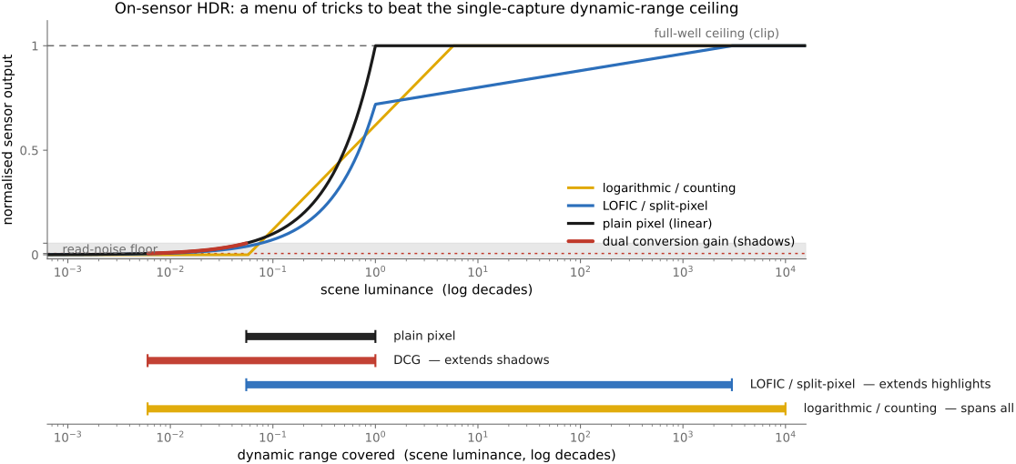
This chapter is about the other route: beat the ceiling on the sensor, within one capture. There is no single trick; there are several hardware options, and the items trade against each other along three axes. Some extend the range at the dark end (lower the effective read noise); some extend it at the bright end (enlarge the effective full well); one compresses the whole range into a non-linear response. Each has a cost in silicon area (an extra transistor, capacitor, or photodiode per pixel), motion robustness (whether the high- and low-range samples are taken at the same instant or not), readout bandwidth, or an SNR dip where two response regimes are stitched together. Figure 34.3.1 lays the menu out as a set of response curves and the slice of dynamic range each one buys.
34.3.1 Staggered / multiple-exposure readout (DOL-HDR)⧉
The most direct idea keeps the linear pixel and simply captures it more than once per frame at different exposure times, reading the array out back-to-back: a long sub-exposure for the shadows and a short one for the highlights, sometimes a third in between, merged on the sensor or by a downstream image processor. In the line-interleaved variant, alternate groups of rows are given long and short integration times so the two sub-images are read in a single pass; in the more general scheme the whole array is read twice in quick succession.
Digital-overlap (DOL) HDR schedules multiple rolling sub-exposures closely and interleaves their output. Output-line overlap does not mean that a given photodiode necessarily integrates two independent charges simultaneously (Figure 34.3.2). Close scheduling can shrink the temporal gap between exposure measurements, and with it the disagreement between them, but it cannot eliminate it. The fundamental cost of any staggered scheme is motion: a fast edge, a passing car, a flickering LED traffic sign sits in different places (or different brightness phases) during the long and short windows, so the two sub-exposures disagree, and the merge leaves a tell-tale artifact along moving boundaries. The second cost is readout bandwidth: reading the array two or three times per frame multiplies the data rate off the chip, which is exactly what the stacked-DRAM architectures of the previous chapter exist to absorb.
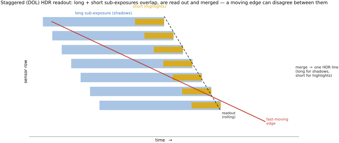
This is, in effect, the multi-frame HDR of HDR merging organized as a high-rate sequence of sensor reads, faster and tighter than a true frame bracket, but heir to the same motion problem, just smaller.
34.3.2 Dual (and triple) conversion gain (DCG)⧉
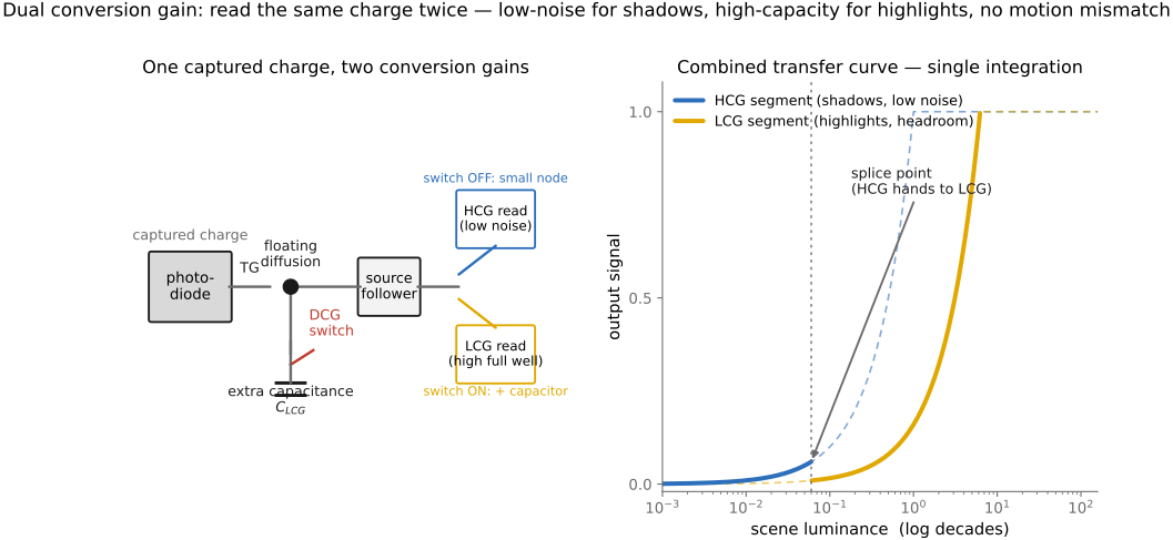
The dominant modern approach, used in flagship smartphones and automotive imaging, sidesteps the motion problem entirely by reading one integration of charge two different ways. The trick lives at the point where the pixel converts collected charge to a voltage: the floating diffusion node, whose capacitance sets the conversion gain (volts produced per electron). A switch transistor adds or removes a small extra capacitance on that node, giving each pixel two modes Li 2008 (dual conversion gain):
- High conversion gain (HCG): small node capacitance, so each electron makes a large voltage step. This swamps the downstream read noise, giving a very low effective read noise ideal for the shadows, but the small node fills up early, capping the highlights.
- Low conversion gain (LCG): the switch adds capacitance, so the node holds far more charge before saturating: more highlight headroom, at the cost of a higher read noise.
Read the same captured charge through both paths and splice them: the low-noise HCG read in the shadows, the high-capacity LCG read in the highlights, and you widen the dynamic range at the dark end, with the highlights protected, all from one exposure (Figure 34.3.3). Because both reads come from the same integration, there is no temporal mismatch at all: nothing moves between them, so DCG is immune to the ghosting that dogs staggered HDR. A camera that switches between the two modes effectively has two native ISOs, one tuned for low noise and one for headroom; the "dual native ISO" marketed on many cameras is DCG underneath. The residual cost is a small SNR dip at the splice point, where the noisier LCG read takes over from the HCG read, plus the per-pixel transistor and capacitor. Pushing further, triple-gain designs add a third conversion-gain (or an overflow reservoir, below) to cover shadows, midtones, and highlights in one shot.
34.3.3 Split-pixel: a large and a small photodiode⧉
Where DCG extends the dark end, the split-pixel (or sub-pixel) design extends the bright end by putting two photodiodes of different size under one pixel: a large, high-sensitivity diode that gathers light efficiently in dim scenes, and a small, low-sensitivity diode (sometimes with its own attenuating filter or micro-lens) that stays unsaturated under direct sun Willassen et al. 2015 (split-diode HDR pixel). The large diode handles the shadows and midtones; the small one, which sees a tiny fraction of the light, carries the extreme highlights long after its big sibling has clipped. Merging the two yields enormous single-capture range.
The decisive application is automotive, where these are sold as LED flicker mitigation (LFM) sensors Oh et al. 2020 (automotive LFM split-pixel). A car's cameras face a brutal combination: headlights and a tunnel exit span an immense contrast, and modern LED tail-lights, signs, and signals are pulse-width-modulated; they flash on and off many times a second. A short exposure (the obvious way to tame the highlights) can fall entirely in an LED's "off" phase, so the sign vanishes from the frame, unacceptable for a driving system. The small photodiode solves both at once: it runs a long integration (so it is more likely to include an LED's on phase; guaranteed coverage requires an integration window long enough for the relevant pulse period) yet stays unsaturated because it is so insensitive. The cost is silicon area (two diodes per pixel) and a tricky calibration of the large gap in sensitivity between them; the highest-range designs combine the split pixel with DCG and an overflow capacitor (next) to read several signals from one pixel.
34.3.4 Spatially-varying exposure (SVE) / assorted exposures⧉
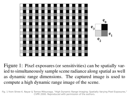
Instead of giving every pixel the same treatment, vary the exposure across the array: neighboring pixels receive different amounts of light, through a patterned neutral-density mask over the photosites or by clocking different pixels for different integration times, so that neighborhoods within the covered radiance range contain usable samples at one or more exposure levels. Saturated and black pixels are then filled in from their better-exposed neighbors, recovering high range from one frame at the price of spatial resolution. This is Nayar and Mitsunaga's spatially varying pixel exposures Nayar & Mitsunaga 2000, the original "assorted exposures" idea and a direct instance of the principle of Chapter 34.1, Assorted pixels (multiplex an extra dimension across the sensor and demultiplex computationally). Its modern incarnation rides on the quad-Bayer mosaic of the previous chapter: give the four same-color sub-pixels of each 2×2 cell different exposure times ("quad-exposure" or per-sub-pixel staggered HDR), folding the HDR multiplexing into the very structure that otherwise bins for low light. The trade-off is the same one every SVE scheme pays: resolution for range, plus the interpolation artifacts of reconstructing a full-resolution image from unevenly-exposed samples.
34.3.5 Lateral overflow integration capacitor (LOFIC)⧉
A different way to extend the bright end refuses to discard the bright charge. As a photodiode nears saturation, the surplus electrons normally spill away and the pixel clips; a lateral overflow integration capacitor (LOFIC) instead provides a second reservoir beside the photodiode into which that overflow charge drains and is stored rather than lost Akahane et al. 2006. At read-out the pixel is sampled twice (a quiet, high-gain read of the photodiode for the shadows, and the overflow capacitor for the highlights) and the two are combined. Large-capacity implementations can reach millions of electrons and dynamic ranges above 100 dB (about 16.6 stops), although these values depend on the pixel design with no bracketing and no motion ghosts. Like DCG, it is a single-integration method, so it is motion-robust; the cost is the per-pixel capacitor's area. LOFIC took hold first in automotive sensors, where flicker and fast motion make multi-shot HDR untenable, and migrated into flagship phone sensors in the mid-2020s, where the newest designs stack LOFIC with DCG (and sometimes a split pixel) to read three or four signals from one pixel and cover shadows, midtones, and highlights together.
34.3.6 Logarithmic, self-resetting, and counting pixels⧉
The final family abandons the linear response altogether and compresses the whole range into the pixel's transfer curve. A logarithmic pixel uses a transistor biased in sub-threshold so its output voltage grows with the logarithm of the photocurrent: a single curve that spans many decades of brightness before reaching its finite output and circuit limits, mimicking the eye's own compressive response (it is the same log front-end used by Chapter 34.7, Event sensors). The catch is poor low-light SNR, slow response in dim scenes, and fixed-pattern noise that is hard to calibrate out of a logarithmic device.
Two related tricks keep a linear (low-noise) response but enlarge the well dynamically. A self-resetting pixel, on the verge of saturating, resets itself and keeps integrating, recording how many times it reset; the true brightness is that count times the well depth plus the final residue, so a small, low-noise well behaves like a much larger one Decker et al. 1998 (wide-DR self-reset pixel). Carried to its limit this becomes a counting pixel: digitize and tally the charge as it arrives, the focal-plane idea taken up by the digital-pixel arrays of Chapter 34.8, Specialized and research sensors. And at the extreme end the count is of individual photons, as in the single-photon and quanta-image sensors of Chapter 34.5, Single-photon sensors (SPAD, avalanche, photon counting), where single-photon sensitivity is possible but dark counts, detection efficiency, and readout or dead-time effects still matter and dynamic range is built up by counting over space and time rather than by deepening a well Fossum et al. (QIS). On-sensor HDR and single-photon imaging meet here: both make a small, quiet detector behave like one with vast capacity, the former by overflow and counting, the latter by tallying photons.
34.3.7 On-sensor HDR versus multi-frame HDR⧉
Step back and the contrast with Multiple exposure imaging is clean. Multi-frame HDR (HDR merging) brackets exposures in time and aligns-and-merges them in software: range extended by the exposure ratios and limited by noise, clipping, flare, and acquisition time, but slow, and fragile to motion unless the alignment is very good. On-sensor HDR captures the range in hardware within one shot: motion-robust (especially the single-integration DCG and LOFIC methods), fast, and cheap in time, but bounded by what the silicon can do and carrying its own artifacts (the staggered methods' residual ghosting, the splice-point SNR dips, the resolution loss of SVE). The two are complementary, not competing, and modern phone pipelines use both at once: an on-sensor HDR read (DCG, often with LOFIC or staggered sub-exposures) supplies each frame of a fast burst, and the burst is then aligned and merged in the style of Chapter 17.6, HDR+ and burst imaging on phones: hardware range per frame, multi-frame range across the burst. The dynamic-range ceiling that once seemed fixed in the photosite is, like the resolution-versus-noise trade of the previous chapter, now partly controlled through acquisition modes selected before and during capture, followed by reconstruction.