33.6 Theoretical analysis of imaging systems in the 4D light field Fourier domain🔗⧉

By this point the part covers many camera designs. There is the pinhole and the lens of Chapter 2.3, Lens Image formation; the focus sweep and the plenoptic camera of Part 31, Light fields and plenoptic cameras; the stereo pair of Chapter 36.1, Multiple view geometry; the coded aperture, wavefront coding, and the lattice-focal lens of the chapters around this one. They look like separate inventions, each with its own trick and its own reconstruction. The thesis of this chapter is that they are one object seen from different angles, and that there is a single place, the Fourier domain of the 4-D light field, where the differences between them become a matter of geometry rather than cleverness, readable almost at a glance.

We have already done half the work. Chapter 6.7, Image formation as a linear system, established the operator view: discretize the scene into a vector $\mathbf{x}$, the image into a vector $\mathbf{y}$, and every camera is a matrix, $\mathbf{y}=A\mathbf{x}+\mathbf{n}$. It also told us the right $\mathbf{x}$ to use if we want one matrix that works for every scene regardless of depth: take $\mathbf{x}$ to be the light field itself (ray space), so that the camera becomes a fixed linear projection of ray space onto the image, with the scene's depth living inside $\mathbf{x}$ rather than inside $A$. Levin, Freeman and Durand drew exactly this picture, and we reproduce it again here because it is the spine of the chapter: every camera is a different projection of the same light field Levin, Freeman & Durand 2008 (Figure 6.7.5⛶ fullscreen).

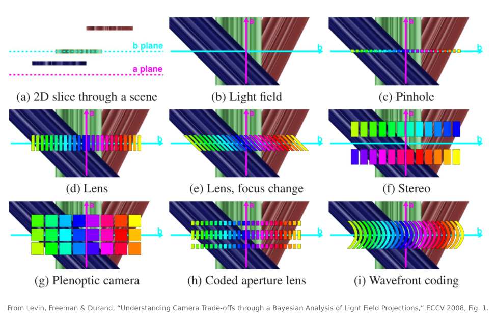
What we add is the second half: once a camera is a linear projection of ray space, many of its resolution, depth-of-field, and reconstruction tradeoffs can be understood through two properties of that projection, the support and the conditioning of its footprint in the 4-D Fourier domain. Support says which parts of the scene's spectrum the camera records at all; conditioning says how strongly it records them, and in particular where it records them so weakly that noise drowns the answer. Their consequences depend on the noise model, the scene prior, and the quantity to be reconstructed. That is the program, and it is the Fourier reading of the operator lesson Chapter 6.7, Image formation as a linear system.

33.6.1 The light field's spectrum, and the one move that explains everything🔗⧉

Begin where the light-field part began: the epipolar slice. Hold a single scene row fixed and lay out the 2-D light field $L(s,u)$: image position $s$ across, aperture position $u$ up. A single scene point, seen from every aperture position, traces a straight line through this slice, and from Chapter 31.1, Light fields 101 we know the result: the slope of that line is the point's disparity, hence its depth. A point on the focus plane has zero disparity and draws a vertical line; a near point and a far point slant opposite ways. Depth is orientation in the epipolar slice. (For a Lambertian point the radiance is the same along the whole line, which is what makes this clean; specular and occluded points are the interesting violations, and we return to them at the end.)

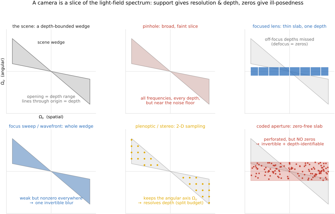
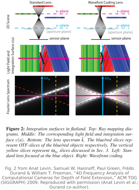
Now take the 2-D Fourier transform of that slice, into a frequency plane with axes $\Omega_s$ (the spatial frequency, conjugate to image position $s$) and $\Omega_u$ (the angular frequency, conjugate to aperture position $u$). A line in the primal domain transforms to a line through the origin in the spectrum, rotated by ninety degrees. A constant-depth slab of the scene, whose every point draws lines of one slope, occupies a single line through the origin of the spectrum, at an orientation set by that depth. Ignoring occlusion boundaries and view-dependent appearance, a scene spans a range of depths, from $z_\min$ to $z_\max$, so its light-field spectrum is a fan of all those lines: a wedge, a double cone, the "bowtie" of Chapter 31.6, Light field aliasing and 4D Fourier analysis (Figure 33.6.1⛶ fullscreen). The wedge's opening angle is set by the scene's depth range: a flat scene at one depth collapses the wedge to a line; a scene running from very near to very far opens it wide. The wedge is the scene's spectral footprint, and every camera in this chapter is competing to record it.

Here is the one move that turns this from a picture into a tool. A camera forms an image by integrating rays over its aperture: summing along the $u$ axis (a focused lens), or along a sheared version of it (a refocused or defocused lens), or sampling rather than summing it (a plenoptic camera). And there is a theorem about what integration does in the Fourier domain, the same projection-slice theorem that powers Fourier-slice refocusing in Chapter 31.4, Refocusing and synthetic aperture and tomographic reconstruction: integrating a signal along one axis in the primal domain is equivalent to taking a slice through the origin along the perpendicular axis in the spectrum. Sum the light field down the aperture and the image you get is, in frequency, a 1-D slice of this 2-D epipolar spectrum, or a 2-D slice in the full 4-D light field. A finite weighted aperture broadens the ideal slice into a spectral weighting. Shear before you sum (refocus) and the slice tilts. So:

the spectrum of the photograph a camera produces is a slice (or, more generally, a slab) of the light-field spectrum, and the camera's design chooses which slice.

Everything else in the chapter is reading off, for each camera, what slice it takes: how much of the scene's wedge that slice covers (support), and how strongly (conditioning).

33.6.2 Every camera is a different slice🔗⧉

With the wedge-and-slab picture in hand, walk the zoo. Each camera is the same projection-slice operation; what differs is the slab.

Pinhole. A pinhole admits one ray per pixel: no integration over the aperture at all. In the spectrum that makes its footprint a broad slice: the ideal geometric pinhole has no defocus dependence. A physical pinhole has finite size and diffraction, so it neither preserves arbitrarily high frequencies nor produces perfect sharpness at all depths. But a small pinhole admits little light: the entire slice sits multiplied by a tiny number, riding down near the noise floor. In conditioning terms a pinhole has broad support but poor signal: every frequency is present but every frequency is noisy. This is the spectral statement of the pinhole's eternal bargain, sharp but dim, from Chapter 2.2, Pinhole Image Formation and linear perspective.

Lens, focused. A full-aperture lens integrates the whole cone of rays converging to a point, a sum down the (possibly sheared) aperture axis. By projection-slice this is a thin slab: at the focal depth it captures the full spatial-frequency content with the lens's whole light-gathering area behind it (bright, sharp), but the slab is narrow in the angular direction, so it lines up with only one orientation of the wedge: one depth. Points at other depths fall outside the slab; their high spatial frequencies are not recorded, which is precisely defocus blur, and worse, the defocus point-spread function of a clear circular aperture has zeros: frequencies it annihilates outright. Those zeros are why naive deblurring of an out-of-focus photo is ill-posed in the exact sense of Chapter 7.1, Imaging as Bayesian inference with probabilistic priors: the operator crushed certain frequencies to nothing, and no inversion brings back what was multiplied by zero. The lens trades the pinhole's universal-but-dim support for a bright-but-depth-bound slab.

Focus sweep and wavefront coding. Now the first piece of cleverness. Suppose that, during one exposure, you sweep the focus through the whole depth range (or use a different mechanism with a similar goal, placing a cubic phase plate in the pupil, as Chapter 33.1, Wavefront coding does). The slab no longer sits at one orientation. It is smeared across the entire wedge. The response at any one depth is weaker than a properly focused lens would give, but it can remain useful over a designed frequency band and depth range, with reduced depth dependence. That is exactly the property that makes wavefront coding's one fixed deconvolution sharpen every depth at once and gives it its extended depth of field. In the spectral picture, sweeping converts a thin slab that covers the wedge richly-but-narrowly into a broad slab that covers it weakly-but-completely, trading peak response for universal, invertible coverage. (The temporal twin is the parabolic sweep of Chapter 6.7, Image formation as a linear system, which does the identical thing to the motion wedge.)

Stereo and plenoptic. Instead of collapsing the aperture axis by integration, keep it: record several aperture positions separately (two, for stereo; a dense grid, for a plenoptic camera). Now the camera no longer takes a 1-D slice; it samples the wedge in two dimensions, recovering the angular axis $\Omega_u$ that the lens summed away. That recovered axis is depth: a system that keeps $\Omega_u$ can tell the wedge's orientations apart, which gives stereo and plenoptic cameras additional evidence for depth and refocusing. Correspondence, texture, occlusions, and angular sampling still constrain recovery. The price is written in the same plane. A sensor has a fixed number of samples, a fixed total area in the $(\Omega_s,\Omega_u)$ plane that it can record, so every sample spent on the angular axis $\Omega_u$ (depth, viewpoint) is a sample not spent on the spatial axis $\Omega_s$ (image resolution). This is the spectral form of the plenoptic camera's notorious spatial-versus-angular resolution trade-off from Chapter 31.2, Light field cameras: the wedge is wide, the budget is fixed, and you choose how to spend it.

Coded aperture. Finally the camera this part is built around. Replace the lens's clear stop with a designed binary mask. The footprint is still a defocus slab, but now its profile is the mask's pattern rather than a smooth disc. The design goal is read straight off Figure 33.6.1⛶ fullscreen: choose the pattern so the slab has no zeros (the target frequencies retain sufficient response for regularized deblurring, subject to noise and the image prior of Chapter 7.1, Imaging as Bayesian inference with probabilistic priors) and so the slab's shape changes recognizably with depth (so that which code best deblurs a patch reveals that patch's depth) Levin, Freeman & Durand 2008. A clear aperture optimizes for neither; a coded aperture is engineered for both. The whole of Chapter 33.3, Coded aperture is the search for the mask whose spectral slab is broad, zero-free, and depth-discriminative at once.

So the zoo collapses. Pinhole, lens, focus sweep, wavefront coding, stereo, plenoptic, coded aperture: one projection-slice operation, seven different slabs across the same wedge. Where a slab covers the wedge broadly you get depth of field; where it keeps the angular axis you get depth; where it stays above the noise with no zeros you get invertibility. The design of a camera is the design of its slab.

33.6.3 Putting cameras on one footing: the Bayesian comparison🔗⧉

The wedge-and-slab picture tells you what each camera records. It does not, by itself, tell you which camera is best, because "best" depends on what you are trying to recover and on how bad the noise is, and because the cameras are not even commensurable at the raw-image level (a plenoptic camera's frames look nothing like a coded-aperture frame). The contribution of Levin, Freeman and Durand Levin, Freeman & Durand 2008 is to make them commensurable, by asking a single question of every camera: given the same noise and the same prior knowledge about scenes, how accurately can you reconstruct the thing you actually want from this camera's measurements?

That is the inverse-problem frame of Chapter 7.1, Imaging as Bayesian inference with probabilistic priors, lifted to compare operators rather than to invert one. Equip the analysis with a prior on light fields (natural images have $1/f$ spectra, scenes have a bounded depth range, so the wedge is the prior's support) and a noise level, and you can compute, for each camera's projection $A$, the expected reconstruction error of the optimal (Bayesian) estimator. This number folds support and conditioning into one verdict: a camera whose slab misses part of the wedge pays for the frequencies it never recorded; a camera whose slab has zeros or near-zeros pays because the prior, not the data, has to supply those frequencies; a camera that records everything but dimly pays in noise. The comparison is fair: every camera is scored by what its measurements let you recover, not by how its raw frames look, which is the only fair way to compare a coded aperture against a plenoptic camera against a plain lens.

The comparison exposes competing demands on finite aperture, exposure, sensor samples, and signal-to-noise ratio. The spectral budget (the area a camera can record above the noise) is finite, and the wedge is fixed by the scene. A camera can spend that budget for spatial resolution (a sharp lens at one depth), or for depth of field (a focus sweep spreading it thin across the wedge), or for depth discrimination (a plenoptic camera keeping the angular axis), but it cannot have all three at full strength, because these goals compete for the same acquisition resources. Spectral area alone is not a universal conservation law for cameras with different sampling and noise models. Coded designs do not break this law; they allocate the budget more cleverly than a clear aperture, which wastes much of its on zeros and on depths it cannot reach. The Bayesian analysis is what lets you see the allocation as a single comparable number, and it is why "which coded camera should I build?" became a question with a principled, rather than a heroic, answer.

33.6.4 The dimensionality gap: most of the 4-D spectrum is afocal🔗⧉

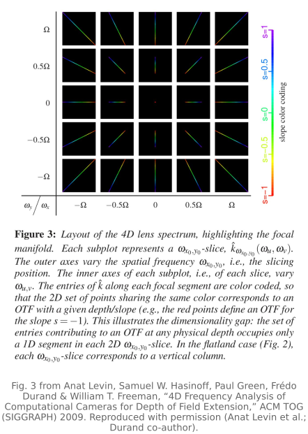
Flatland has served us well, and it hides exactly one thing: the fact the best design of this part is built on. Go back to the full 4-D light field. The rays leaving one scene point form a 2-D plane in ray space, and because the point sits at a single depth, that plane's slope in the $x$-$u$ pair equals its slope in the $y$-$v$ pair: $s_u=s_v$. Within this axis-aligned family, the two slopes can vary independently; a general 2-D plane in 4-D has additional degrees of freedom. The planes with $s_u\neq s_v$ correspond to no scene point at any depth; they are the ray geometry of astigmatic surfaces, the reflection off a cylindrical mirror for instance, and a Lambertian scene puts nothing there. Count dimensions: equal-slope planes form a 3-D family (one slope, two offsets), all planes a 4-D one. The focal manifold occupies a 3-D subset of the 4-D frequency domain in this model. Occlusion and view dependence can spread scene spectra outside the idealized support. This is the dimensionality gap Levin et al. 2009 (4D frequency / lattice-focal), and it is invisible in flatland, where there is only one slope to have. That is why this section, alone in the chapter, needs all four dimensions.

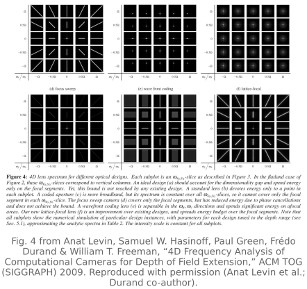
In the Fourier domain the gap becomes a picture you can design against (Figure 33.6.2⛶ fullscreen). Take the camera's 4-D spectrum $\hat k(\omega_x,\omega_y,\omega_u,\omega_v)$, fix a spatial frequency $(\omega_{x_0},\omega_{y_0})$, and look at the 2-D slice that remains, with axes $(\omega_u,\omega_v)$. By projection-slice, the OTF at depth slope $s$ reads off the single point $(\omega_u,\omega_v)=(-s\,\omega_{x_0},-s\,\omega_{y_0})$. Sweep $s$ across the depth range and that point sweeps a 1-D line segment, the focal segment. Every photograph the camera can take, at this spatial frequency, at any depth, reads from that segment; the rest of the 2-D slice is afocal, spent on the astigmatic ray combinations no photograph uses.

The design principle follows at once: the energy a lens can put into each slice is finite (the next sections make the budget exact), so an ideal design spends it on the focal segments and nowhere else. Reread the zoo with this sharper eye. A standard lens puts everything on one point of the segment, its focus depth, and covers no other. A coded aperture is broadband, but its spectrum is the same in every slice, and the segment's orientation rotates from slice to slice, so no single pattern can track it: a large share of its budget is provably afocal. Wavefront coding is separable in $u$ and $v$, so it fills the axis-aligned rectangle that bounds the segment; off the diagonal the cubic surface is locally astigmatic, and that part of the rectangle is afocal too. The focus sweep alone stays on the segment, but phase cancellation between its focus settings keeps the magnitude low. Naming what each design wastes is what points at a better lens.

33.6.5 The lattice-focal lens: tiling the wedge🔗⧉

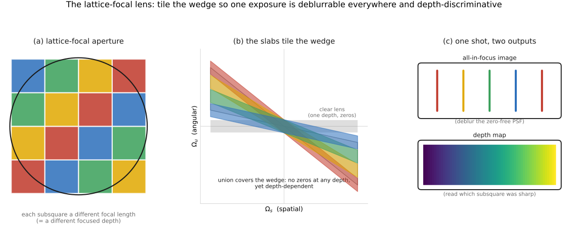
The cleanest payoff of taking the analysis seriously is a lens that the analysis essentially designed. Start from the depth-from-defocus goal: capture one image from which you can recover both an all-in-focus picture and a depth map. The spectral requirement, read off Figure 33.6.1⛶ fullscreen, is demanding: you want a single PSF that, at every depth in the range, is both well-conditioned (no zeros, so you can deblur) and depth-discriminative (different enough across depths that you can tell them apart). A clear lens fails on both counts: at each depth it is sharp in one band and zeroed elsewhere, and its defocus changes only slowly and ambiguously with depth. A focus sweep is well-conditioned but deliberately depth-invariant, which is the opposite of what depth-from-defocus needs.

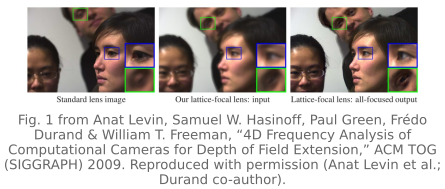
The lattice-focal lens of Levin, Hasinoff, Green, Durand and Freeman Levin et al. 2009 (4D frequency / lattice-focal) resolves the tension by tiling the aperture: it is a mosaic of subsquares, each ground to a different focal length. Each subsquare brings a different depth into sharp focus, so for any depth in the range some subsquare images it crisply, contributing the high spatial frequencies that depth would otherwise lose. The union of the subsquares' responses covers the whole wedge with no zeros at any depth (every depth has a sharp sub-image somewhere in the mosaic), while the identity of which subsquare is sharp makes the PSF strongly depth-dependent, so depth is recoverable. In the spectral picture the lattice-focal lens tiles the wedge: where the focus sweep smeared one slab thinly across all depths, the lattice-focal lens lays down a patchwork of slabs that together blanket the wedge with good conditioning and keep the depth signature the sweep threw away (Figure 33.6.3⛶ fullscreen). And in the 4-D picture of the previous section it obeys the dimensionality gap by construction: every tile is a piece of an ordinary lens, its slopes in $u$ and $v$ equal, so the whole aperture is focal, where wavefront coding's cubic surface is astigmatic almost everywhere. It is, in one fixed piece of glass and one exposure, what a focus sweep achieves over time, but with the depth information preserved.

How big should the tiles be? That is the design's one free parameter, and the analysis fixes it. A subsquare of width $\epsilon A$ behaves like a small lens: a narrow aperture, hence a wide depth of field of its own. It keeps its target depth acceptably sharp (defocus under a pixel) over a band of neighboring depths, and the band widens as the subsquare shrinks. Too few large subsquares and the bands fail to cover the range: some depths get no sharp contributor. Too many small ones and the bands overlap redundantly while each contributes a dimmer, more spread response. The optimum has every depth covered by exactly one subsquare, which works out to $\epsilon^{*}=(AS\Omega_{\max})^{-1/3}$, where $A$ is the aperture width, $S$ the slope range covered, and $\Omega_{\max}$ the highest spatial frequency the sensor records Levin et al. 2009 (4D frequency / lattice-focal). At the paper's operating point (an aperture about a thousand pixels wide, slope range $S=2$) that means roughly a hundred subsquares; the prototype, plano-convex elements sawed into 12 squares and mounted like a filter on an 85mm lens, could therefore cover only a modest depth range.

Why does spending aperture beat spending exposure? Compare against a focus sweep chopped into $N$ discrete focus settings. Each of the sweep's time bins uses the full aperture for $1/N$ of the exposure; each lattice tile uses $1/N$ of the aperture for the full exposure. The light collected per bin is identical. The difference is the depth of field of each bin: the sweep's bins are full-aperture lenses, sharp over a sliver of depth, while the lattice's tiles are narrow-aperture lenses sharp over a band $\sqrt N$ times wider. Summed over bins, the lattice therefore holds more spectrum at every depth than the sweep. That is the entire advantage, made exact by the numbers of the next section.

33.6.6 The upper bound, and the gap we have not closed🔗⧉

The lattice-focal lens is a good design, but "good" only sharpens the question the 2009 analysis was really built to answer: how good could any camera be? The ceiling comes from conservation of energy. Over a fixed exposure, a clear aperture of width $A$ passes unit energy through each of its points; push that through Parseval and the power a lens spectrum can hold on the focal segment of any slice is capped at $A^3$. The segment has length $S|\omega|$ at spatial frequency $\omega$: it lengthens with the depth range and with frequency. The best any design could do for the worst depth is spread the budget evenly along it Levin et al. 2009 (4D frequency / lattice-focal):

(up to a geometry factor within 7% of 1). In words: the upper bound on worst-depth power falls inversely with spatial frequency, and grows as the cube of the aperture. No design within the analysis's fixed-aperture, fixed-exposure model exceeds this worst-depth bound over the range. It is the depth-of-field analog of a diffraction limit: a statement not about a particular lens but about the response attainable under these acquisition and scene assumptions (Figure 33.6.5⛶ fullscreen).

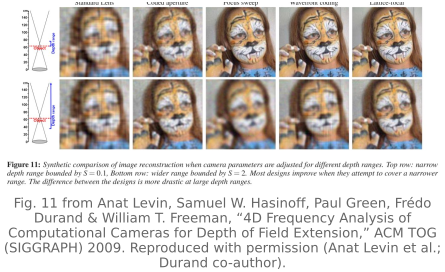
Against this ceiling the paper scores every design in closed form, and the exponents are the verdict. A standard lens focused at $s_0$ gives $|\hat\phi_s|^2=A^4\,\mathrm{sinc}^2\!\bigl(A(s-s_0)\omega_x\bigr)\,\mathrm{sinc}^2\!\bigl(A(s-s_0)\omega_y\bigr)$: enormous in focus, collapsing away from it. The two depth-invariant designs land at $|\hat\phi_s|^2\approx A^2/(S^2|\omega_x||\omega_y|)$ for wavefront coding and $\approx A^2/(S^2|\omega|^2)$ for the focus sweep: quadratic falloff, aperture only squared. The lattice-focal lens with the optimal tile size reaches $|\hat\phi_s|^2\approx A^{8/3}/(S^{4/3}\Omega_{\max}^{1/3}|\omega|)$: linear falloff like the bound, with $A^{8/3}$ in place of $A^3$. Two ratios summarize it. Lattice-focal over wavefront coding is about $(AS\Omega_{\max})^{2/3}$ at the cutoff frequency: at the paper's operating point ($AS\Omega_{\max}\approx 1000$) roughly a hundredfold in power, a tenfold MTF, and the margin grows with frequency because the falloffs differ. Bound over lattice-focal is $(AS\Omega_{\max})^{1/3}$: one order of magnitude, at every frequency. Both facts show in the plotted spectra (Figure 33.6.5⛶ fullscreen) and in the reconstructions (Figure 33.6.7⛶ fullscreen). One caveat: the advantage is asymptotic in the depth range. Over a narrow range the focal segment barely exceeds its bounding rectangle, wavefront coding wastes almost nothing, and the designs nearly tie; the 12-subsquare prototype lived mostly in that regime.

So in 2009 the best single-shot camera sat one order of magnitude below the upper bound, which need not be attainable. Which is wrong, the design or the bound? The authors suspected the bound: its proof lets the full $A$-wide aperture serve every depth at once, but covering a range of slopes forces disjoint pieces of aperture per depth, each with a smaller support and hence a thicker, weaker spectral footprint. Baek turned that suspicion into theorems the following year Baek 2010 (transfer efficiency vs depth invariance). He showed that the OTF at a fixed spatial frequency, viewed as a function of defocus, has a Fourier transform confined to a small trapezoid, and from this structure derived tighter bounds on the depth-averaged spectrum in that analysis, below the 2009 ceiling. More useful than the tighter constant is the tradeoff he proved: transfer efficiency (how much spectrum you keep) and depth invariance (how little the blur changes with depth) pull directly against each other, and both cannot be had. Among designs with a fully depth-invariant OTF the focus sweep is already near-optimal; for a depth-invariant MTF at any single chosen frequency, a tuned cubic phase plate is; and Baek conjectures that no one lens is optimal at every frequency at once. The lattice-focal lens does not contradict this: it buys its extra order of magnitude by giving up depth invariance, which is why it must estimate depth before it can deblur (and returns a depth map as a bonus). The remaining gap identified by these analyses is: the exact worst-case ceiling for depth-dependent single-shot designs, somewhere between the lattice-focal's $A^{8/3}$ and the energy bound's $A^3$.

33.6.7 From cameras to light transport: the same spectral lens🔗⧉

The reach of this analysis does not stop at the camera. The camera is only the last interaction in a long chain: light leaves a source, travels across empty space, gets occluded by silhouettes, reflects off surfaces, passes through a lens, and finally lands on the sensor. Each of those interactions is an operation on the same 4-D radiance signal, and Durand, Holzschuch, Soler, Chan and Sillion showed that each one has a clean, predictable effect on its spectrum Durand et al. 2005 (frequency analysis of light transport). The camera analysis is one instance of a far more general frequency analysis of light transport.

The vocabulary is the same slice/shear/wedge algebra, now applied interaction by interaction. Travel across a distance is a shear of the light field (the same shear that refocusing applies) so it shears the spectrum's wedge without adding or removing energy. Occlusion multiplies the radiance by a silhouette's binary mask, and multiplication in the primal domain is convolution in the spectrum: a sharp occluder edge has broad spectral content, so occlusion spreads the signal's bandwidth, injecting high frequencies (this is why shadow boundaries and silhouettes are where rendered images need the most samples). Locally, under the paper's reflection parameterization and approximations, glossy reflection acts like an angular convolution with the BRDF, and convolution by a smooth kernel is a low-pass filter: a Lambertian surface has outgoing radiance independent of direction (away from visibility changes), a mirror passes everything. Lens defocus, at the end of the chain, is the integration-and-slice we have spent the whole chapter on. Curvature reshapes the wedge; the cosine and distance falloffs rescale it.

The practical payoff of tracking all this is that you can predict the local bandwidth of radiance at every point of a scene, and bandwidth is a sampling rate. Where transport has band-limited the signal (a matte surface seen through a wide defocus), you can afford to sample sparsely and interpolate; where it has injected high frequencies (a sharp shadow on a textured wall, a glossy highlight), you must sample densely. This is the basis of adaptive sampling in rendering, and it closes the loop with the camera side: the camera's slab and the scene's wedge are two ends of the same signal, reshaped by the same shears and convolutions, and "what does this optical system do to the signal?" is, from light source to pixel, one spectral question with one consistent answer. It is also the natural bridge to the sampling sibling, Chapter 31.6, Light field aliasing and 4D Fourier analysis, which asks the dual question (given this wedge, how densely must I photograph it to avoid aliasing?) using the very same spectral support that here told us how densely a camera records it.

33.6.8 Where this leaves the part🔗⧉

Step back and the chapter has done one thing: it has turned the qualitative slogan of Chapter 6.7, Image formation as a linear system (a camera is a linear projection of the light field) into a quantitative instrument. Drop a scene into the 4-D Fourier domain and it is a wedge whose opening is its depth range. Drop a camera in beside it and it is a slab, a slice of that wedge chosen by the optics. Read the slab's support and you have the camera's resolution, depth of field, and ability to discriminate depth; read its conditioning (including small nonzero responses as well as zeros) and you have its invertibility and its noise behavior, the Chapter 7.1, Imaging as Bayesian inference with probabilistic priors verdict made spectral. The Bayesian analysis folds both into a single comparable number, so cameras can be ranked rather than merely admired Levin, Freeman & Durand 2008; the no-free-lunch conservation law says the spectral budget is finite, so coded designs win by allocating it, not by escaping it; and the lattice-focal lens Levin et al. 2009 (4D frequency / lattice-focal) is one example of a good allocation in hardware, a tiling of the wedge that no clear aperture could manage. The 4-D frequency analysis goes one step further and computes the upper bound on that allocation (the best depth-of-field response any camera could achieve) and shows that even the lattice-focal lens sits an order of magnitude below it. Baek's tradeoff theorems then locate the gap Baek 2010 (transfer efficiency vs depth invariance): depth invariance itself costs spectrum, the sweep and the cubic plate are near-optimal among designs that keep it, and these analyses leave a gap between the best constructions and the upper bound for designs that give it up. The same spectral lens, pulled back along the light path, governs transport itself Durand et al. 2005 (frequency analysis of light transport). Every coded camera in the chapters around this one is a particular answer to one question this chapter has now made precise: which slab of the wedge should I record, and how do I keep it conditioned?