31.7 Lumigraph and shape priors for sharper light field rendering🔗⧉

We ended Chapter 31.1, Light fields 101 with a renderer that felt almost too good. To synthesize a photograph from a viewpoint the camera never physically occupied, you do not model the scene at all: for each output pixel you trace its ray, find where that ray pierces the aperture plane $(u,v)$ and the image plane $(s,t)$, and read off the stored radiance $L(u,v,s,t)$. No surfaces, no depth, and no geometry; the renderer uses the rays directly, and a new view is a lookup. This is pure light-field rendering Levoy & Hanrahan 1996, and sufficiently dense samples can approximate it well within their captured ray coverage.

The trouble is the word densely. You never have the exact ray you want. The output ray almost always pierces the two planes between the rays you actually recorded, so you must interpolate among the nearest stored samples, and interpolation is only as good as the spacing of the samples it blends. Capture a tight grid of views and the in-between rays you need are near neighbors that genuinely agree, so the blend is sharp. Capture a sparse grid, that is, a handful of views over a wide baseline, which is what any practical rig gives you, and the rays you blend belong to scene points at different depths that have moved by different amounts between views, so averaging them is averaging the wrong things. The result is the failure we flagged at the end of Chapter 31.1, Light fields 101: a soft blur where the field is barely under-sampled, and outright ghosting, a faint double image, where it is badly under-sampled. Pure light-field rendering has no scene model, so when the rays run out it has nothing to fall back on, and it guesses. Why this is exactly aliasing, and how much sampling it takes to avoid, is the business of Chapter 31.6, Light field aliasing and 4D Fourier analysis; this chapter is about the practical cure that chapter then justifies.

The cure is to stop pretending we know nothing about the scene. We almost always have, or can cheaply estimate, an approximate shape such as a rough depth map, a visual hull, or a coarse mesh. A sufficiently accurate geometry proxy can greatly reduce blur by selecting corresponding surface samples before blending. That is the Lumigraph Gortler et al. 1996, and the reason it works is the spine of this chapter.

31.7.1 Pure light-field rendering blurs because it has no shape🔗⧉

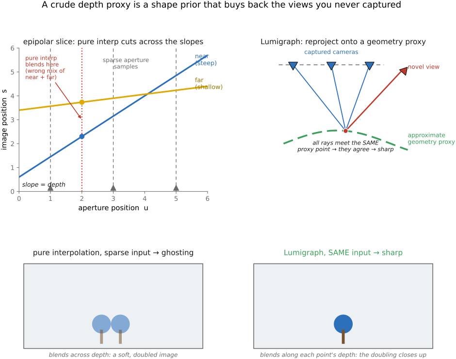
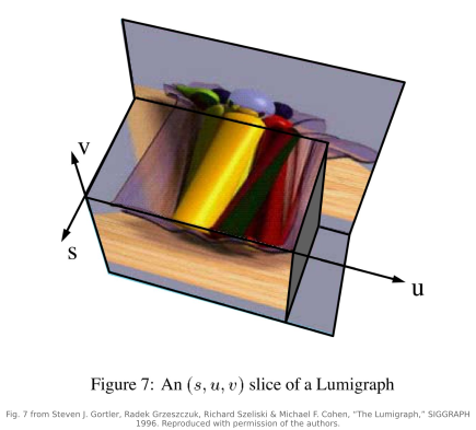
The ray-space picture of Chapter 31.1, Light fields 101 makes the cure obvious. Recall the epipolar slice: fix a scene row and plot image position $s$ against aperture position $u$. A single scene point traces a straight line, and the line's slope is the point's depth: near points lean one way, far points another. The full light field is a dense thicket of these lines; rendering a new view amounts to reading values along a path through the slice.

Now sample the aperture coarsely, keeping only a few columns of $u$. Between two kept columns, a near point's line has marched a long way across $s$ (its slope is steep) while a far point's line has barely moved. Pure interpolation, knowing none of this, blends the two kept samples as if the value varied linearly in $u$, which ignores the depth-dependent shift. A zero-disparity plane has constant image position under the chosen parameterization; it need not be at infinity. For everything closer, the true in-between value sits at a sheared position the interpolation never visits, so it averages a foreground sample with a background one and you get a blur; push the spacing further and the two contributions separate into a visible double image, the ghost. The defect is not noise or a bad blend kernel. It is that the interpolation walks straight up the $u$ axis when the data run along sloped lines. The slope it is ignoring is exactly depth (Figure 31.7.1⛶ fullscreen).

So the missing ingredient has a name. If we knew each point's depth (the slope of its line) we could follow the line instead of cutting across it, blending the right samples. We do not need the depth to be exact; we need it to be close enough that the samples we end up blending belong to the same scene point. That is a weak, forgiving requirement, and it is what makes the prior cheap.

31.7.2 The Lumigraph: reproject onto a geometry proxy, then blend🔗⧉

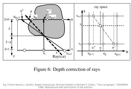
The Lumigraph's move is depth-corrected interpolation Gortler et al. 1996. Alongside the recorded rays it carries an approximate geometry proxy, in the original work a coarse polygonal model recovered from the object's silhouettes (a visual hull); in modern practice, any rough depth map or mesh. To render an output pixel, you no longer interpolate in the abstract: you trace the output ray, intersect it with the proxy surface to get an estimated 3-D scene point, and then ask each nearby recorded camera, what color did you see at that same point?, by projecting the point back into that camera and reading its pixel. You blend those values.

The difference from pure rendering is entirely in which samples get averaged. Pure rendering blends rays that merely pass near the desired ray in the four-dimensional two-plane coordinates; the Lumigraph blends rays that all strike the same estimated surface point, gathered from different directions. If the proxy is even roughly right, those rays are genuinely views of one scene point, so they agree, and their average is sharp instead of smeared. In the epipolar-slice picture, reprojection is the act of shearing the blend to follow the line's slope rather than cutting vertically across it: the proxy supplies the slope, the interpolation rides along it, and the ghosting closes up. A wrong proxy can produce blur, double edges, or visibility errors rather than a simple proportional degradation, because a point at the wrong depth reprojects into each camera at a slightly inconsistent place. This robustness is why "approximate" is enough.

Two practical pieces complete the recipe, both concern the blend weights, that is, how much each captured camera contributes to a reprojected point. First, you weight by angular proximity: a camera whose viewing direction is closest to the desired output ray's direction should dominate, because it is the most faithful witness of any view-dependent shading at that point; cameras at glancing angles contribute less. Second, you must respect visibility and field of view: a camera that never saw the point, because it was occluded or fell outside that camera's frame, must get zero weight, and the weights must vary smoothly so that a camera fading in or out as you move the viewpoint does not pop. The Lumigraph handled the structured, gridded case; getting these weights right in general is precisely what the unstructured successors below are about.

The result is a direct trade between geometry and number of views. With no geometry you need a dense grid to render sharply; with a good proxy you render the same sharpness from a handful of cameras. This is the dual statement of the plenoptic-sampling theorem you will meet in Chapter 31.6, Light field aliasing and 4D Fourier analysis, which says the maximum allowable view spacing for alias-free rendering depends on the scene's depth range, and can be relaxed when useful geometry reduces residual disparity uncertainty. The Lumigraph spends a cheap shape prior to buy back expensive samples; everything that follows is about making the prior cheaper to get, looser to require, or richer to exploit.

31.7.3 Unstructured inputs: free-hand views, no grid required🔗⧉

The Lumigraph as stated assumes cameras on a regular plane and grid, that is, the two-plane parameterization taken literally. Real capture is messier and far more convenient: you wave a phone around the object, grabbing dozens of overlapping shots from wherever you happened to stand, and recover each shot's pose afterward by structure-from-motion. The views are now an irregular cloud in space, not a lattice, and the gridded blend no longer applies. Making depth-corrected rendering work from such inputs is the problem of unstructured light-field rendering, and it is where the blend-weight machinery hinted at above does the real work.

The unstructured lumigraph Buehler et al. 2001 answers it by defining, for any desired output ray, a principled blend weight for each captured camera, computed from a few intuitive penalties and designed to degrade gracefully toward both of its parents. The dominant term is angular deviation: prefer the captured rays whose direction is closest to the desired ray, since they best match the desired view. In the dense-grid limit, this is the term that reproduces ordinary light-field rendering. Added to it are penalties for resolution (prefer a camera that saw the point at adequate sampling, not a distant one whose pixel covers a huge patch) and for field-of-view (a camera contributes zero once the point leaves its frame, and the weight must ramp to zero smoothly so views fade in and out without popping). A camera that cannot see the point, because it is occluded by the proxy, is excluded. The blend is then a normalized, smoothly varying combination of the few best-placed cameras, evaluated per output ray. The result is a single renderer that spans the whole spectrum: hand it a dense planar grid and it behaves like light-field rendering; hand it a sparse set with good geometry and it behaves like the Lumigraph; hand it anything in between and it interpolates between the two regimes by construction. It still leans on a geometry proxy (the shape prior never leaves), but it no longer cares how the cameras were arranged.

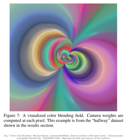
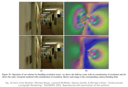
A second answer drops the global proxy almost entirely. Unstructured light fields Davis et al. 2012 render directly from a free-hand, irregularly sampled set of views by leaning on the chapter-before's machinery instead of an explicit mesh. The idea: treat every captured image as a sample on a (warped) camera plane, and reconstruct a new view the way you refocus, with a focal-stack-style sweep. Recall from Chapter 31.4, Refocusing and synthetic aperture that refocusing is shift-and-add: pick a depth, shift each view by the parallax that depth implies, and sum; the chosen depth comes into sharp agreement while the rest blurs. Run that sweep over a range of depths at every output pixel and, exactly as in focus stacking, keep the depth at which the local agreement is sharpest: the views reinforce one another only when shifted by the right parallax, so the sharpest-agreement depth is, in effect, a per-pixel geometry estimate discovered on the fly. There is no global mesh to build or get wrong; the "proxy" is recomputed locally and implicitly from the data itself, which is what lets the method run on a casual, unstructured capture without requiring a global mesh, though camera calibration/pose recovery and local depth inference are still required. It is the same shape prior as the Lumigraph's, but inferred per pixel from focus rather than supplied up front. This is the rendering-side echo of the depth-from-focus read-out of Chapter 31.4, Refocusing and synthetic aperture.

Both methods are downstream of one older, foundational insight from outside the light-field literature proper: view-dependent texture mapping Debevec et al. 1996 (Façade). Reconstructing a building from photographs, Debevec, Taylor and Malik had an approximate geometric model (a coarse architectural mesh) but knew that a single flat texture painted on it would look dead: flat textures cannot reproduce the way real surfaces change with viewpoint (a glint here, a darkened recess there, the subtle parallax of a relief the mesh did not model). Their fix was to keep several photographs as textures and, when rendering a new view, blend them weighted by how close each source camera's direction is to the new view's, so the texture you see is mostly the photo taken from nearest your current vantage, and it slides smoothly to the next as you move. That is the angular-blend idea in its first dress: geometry handles the parallax (where things are), photographs handle the appearance (what they look like from here), and the two are combined by directional weights. The unstructured lumigraph is, in a real sense, view-dependent texture mapping with the weighting made principled and general. Hold onto the division of labor (geometry for parallax, captured images for view-dependent appearance) because the next section pushes it to its limit.

31.7.4 Surface light fields🔗⧉

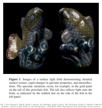
Every method so far carries the appearance as a stack of captured images and uses geometry only to know where to look them up. The surface light field inverts the emphasis: it assumes you already have accurate geometry (a real mesh, from a laser scan or multi-view stereo) and asks, what is the most natural thing to store on top of it? The answer is to parameterize the outgoing radiance directly on the object's surface: at every surface point, record a small function of viewing direction giving the color that point sends each way Wood et al. 2000 (surface light fields). Not one color per point (that is a view-independent appearance texture, which cannot by itself reproduce changing specular reflections), but a whole little lobe of color-versus-direction at each point.

This is the extreme of "geometry as a prior." Here is why it is so economical. With exact geometry, all the parallax is explained by the surface: as you move the camera, where each point appears is computed exactly by projecting the known mesh, so none of your stored data has to encode it. What is left over is only the part a texture genuinely cannot capture: how a point's color changes with viewing angle, a moving specular highlight, a glossy sheen, a faint reflection of the surroundings that slides as you orbit. A single texture is forced to pick one color and so renders a shiny pot as a dull one; the surface light field stores the angular lobe and renders the highlight sliding across the surface as the view turns, which is exactly what your eye expects from a real glossy object (the figure). Because the geometry has absorbed the parallax, many surfaces have compressible angular appearance. Sharp reflections or complex visibility can require much denser directional sampling; known geometry does not guarantee a smooth angular function. Light field mapping Chen et al. 2002 (light field mapping) is the practical realization: it factors the per-point angular function into a few terms that map onto standard texture-mapping hardware, so a surface light field renders in real time as a handful of blended texture passes. The name says it precisely: it is a light field mapped onto the surface rather than indexed by two abstract planes.

Step back and the surface light field is the natural endpoint of this chapter's progression. We began with no shape prior (pure light-field rendering, which blurs), added an approximate one (the Lumigraph and its unstructured kin, which sharpen), and now use an exact one. At that point the only thing worth storing is the view-dependent appearance the geometry cannot explain. Pushed one notch further, that outgoing-radiance function records the result of reflectance under the captured illumination. It does not by itself determine the BRDF or predict arbitrary relighting, which connects surface light fields to reflectance fields and the BRDF, and to the modern neural appearance models that learn a compact view- (and light-) dependent function over a known or jointly recovered shape. The dividing line throughout has been the same: how much of the image is explained by geometry (a prior you supply or infer) versus stored radiance (data you must capture). Make the geometric prior richer and the data shrink. The richest, most flexible prior is one you learn, which is where light fields meet neural rendering in Chapter 31.9, Light field networks.