30.6 Video stabilization and rolling-shutter correction🔗⧉

The previous chapters made motion an enemy to estimate (optical flow) or a cue to track (KLT). Here motion is the thing we want to edit. Hold a phone and walk, and the footage carries an involuntary, high-frequency tremor riding on top of whatever motion you intended, the slow pan, the deliberate hold. A shaky video, in other words, is a good video plus an unwanted signal, and that signal lives on the camera path: the trajectory the camera swung through over the course of the clip. Stabilization is the act of subtracting it.

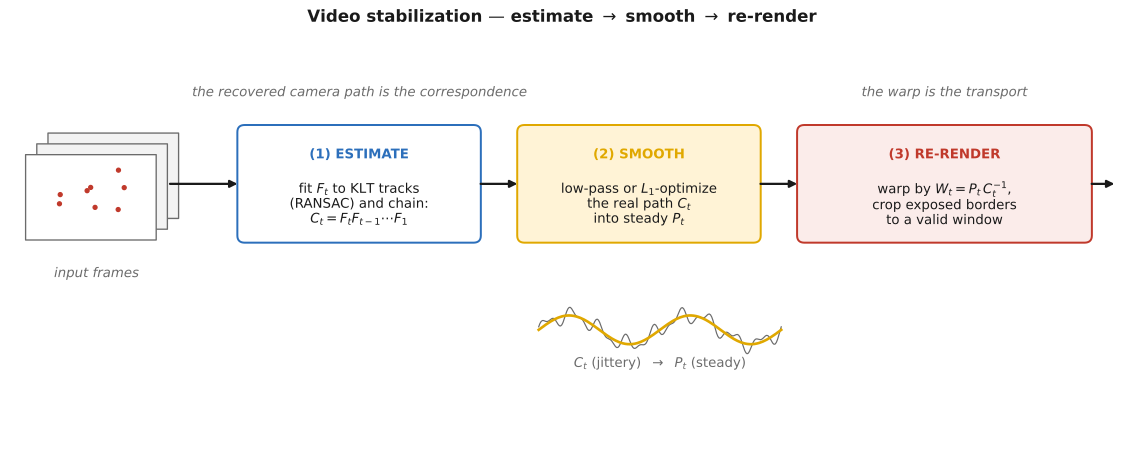
Every method in this chapter is one pipeline: measure the real path, design a better path, warp the frames onto it. Measure the jittery trajectory the camera actually followed; design the smooth trajectory a tripod, dolly, or Steadicam would have produced instead; then re-render each frame by warping it from where the camera was to where the smooth path says it should be. An immediate cost is the border pixels that the better path no longer sees, which must be cropped away or inpainted back. That tension, between how much shake you remove and how much frame you keep, is a central tradeoff, alongside latency, geometric distortion, and residual motion blur, and we will name it precisely.

There is a second lesson underneath, recurring rather than new. Stabilization is temporal signal processing on the camera-path signal, and the same Nyquist intuition from resampling applies: we low-pass the trajectory to strip the jitter while keeping the intended motion, exactly as we low-pass an image before downsampling it. Rolling-shutter "jello," when we reach it, is the time-axis sampling problem within a single frame (rows captured at different instants under fast motion), a loose echo of the L16 sampling lesson rather than a strict instance of it.

30.6.1 What stabilization is: a camera-path signal to be smoothed🔗⧉

The framing is the whole chapter in miniature. The recorded video equals an intended camera motion (a slow pan, a hold) plus an unwanted high-frequency tremor, and that tremor is a signal living on the camera path. Stabilization removes the tremor without removing the intended motion, which is to say it is a low-pass filter on the trajectory. Two subtleties keep it from being a one-line exercise: the "samples" we are filtering are not scalars but 2-D image transforms (a homography per frame, or its parameters), and we cannot let the filtered frame swing so far that it crops away the whole picture.

That gives the chapter's three stages:

1. Estimate the per-frame camera motion and accumulate it into a trajectory.
2. Smooth that trajectory into the steady path a tripod or dolly would have followed.
3. Re-render each frame by warping it from its real pose to the smoothed pose, then crop or inpaint the exposed borders.

One fact makes the whole enterprise tractable without any 3-D reconstruction. For a purely rotating camera, or for a planar scene under the pinhole model, the motion between frames is a homography. A distant scene permits a useful approximation when translation is small relative to scene depth. In these cases we use the same "depth doesn't matter for a rotation or a plane" fact that lets a panorama reproject onto a common surface (cross-ref Chapter 20.2, Automatic panorama stitching from multiple views and feature matching). And most handheld shake is dominated by rotation: a trembling wrist rocks the camera far more than it translates it. So a 2-D motion model already does the heavy lifting. The hard case is genuine translation through a 3-D scene, where near and far objects parallax past each other at different rates. This is the one that breaks the single-homography assumption and needs the content-preserving warps we reach in Stage 2 (Figure 30.6.1⛶ fullscreen).

30.6.2 Stage 1: estimating the camera trajectory🔗⧉

To recover the path, we work locally and then accumulate. Between two consecutive frames, fit a global 2-D transform $F_t$ to a set of point correspondences. The transform comes in increasing fidelity: a pure translation is the crudest model, an affine map adds rotation/scale/shear, and a full homography captures the perspective of a rotating camera; you pick the simplest one that fits your footage. The correspondences themselves come from KLT feature tracks or matched corners (cross-ref Chapter 12.4, Feature tracking): a good corner is trackable for the same reason it is a good keypoint, which is why the tracking chapter feeds directly into this one.

The one defensive measure that matters is robust fitting. A moving foreground object, a person walking through the shot, drags its own feature tracks along with it, and if those tracks enter the fit they will pull the estimated camera motion toward the object's motion. So we fit $F_t$ with RANSAC, exactly the robust-homography machinery from automatic panorama stitching: sample a minimal set, count inliers, keep the consensus, and reject inconsistent tracks. If the moving object dominates the features, RANSAC can instead select its motion; masks, spatial coverage, or inertial measurements can help identify the background (cross-ref Chapter 20.2, Automatic panorama stitching from multiple views and feature matching).

With the inter-frame transforms in hand, chain them into an absolute trajectory:

The camera path is now a sequence of transforms, or, if you parameterize it, a multi-dimensional time signal: translation in $x$ and $y$, rotation, scale, and so on, each a 1-D curve over the clip. This is the object we will smooth.

The catch to name is drift. Every $F_t$ carries a small estimation error, and chaining accumulates those errors, so $C_t$ slowly wanders away from the truth; the same error-accumulation that bundle adjustment corrects in panoramas and structure-from-motion. For a finite clip the drift is usually tolerable; long sequences want global optimization or loop closure to pin it down.

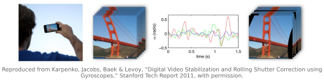
There is a sensor-side alternative that sidesteps feature tracking entirely. Rather than estimate the camera's rotation from pixels, read it from the phone's gyroscope: Karpenko, Jacobs, Baek and Levoy (2011) integrate the gyro signal to obtain the camera's rotation directly. It is cheap, robust to scene content (no features to lose on a blank wall), and it is exactly the per-instant rotation that rolling-shutter correction will also need at the end of the chapter. Hold that thread; it is where the gyro is most useful (Figure 30.6.2⛶ fullscreen).

30.6.3 Stage 2: smoothing the path (low-pass vs. L1-optimal cinematic paths)🔗⧉

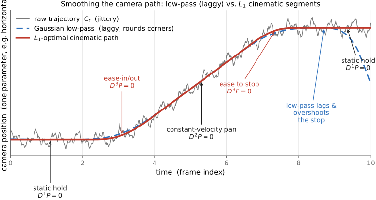
Now we design the better path $P_t$. The obvious move is naive low-pass smoothing: smooth a suitable parameterization of the trajectory with a temporal Gaussian. Writing this componentwise operation schematically,

with Gaussian weights $g_k$. It is simple and it does remove jitter, but it has three real failings. A causal smoother lags. A centered positive Gaussian does not inherently overshoot a scalar step, but it spreads the start and stop of a pan across time. It blurs intended motion, because a fixed kernel cannot tell a deliberate whip-pan from a tremor; both are "fast," so both get attenuated. And to avoid lagging it needs future frames, making it acausal; fine for offline processing, awkward for live preview (Figure 30.6.3⛶ fullscreen).

The deeper idea, due to Grundmann, Kwatra and Essa (2011), is to stop smoothing and start synthesizing: produce the path a professional camera operator would have shot. A trained operator's footage is built from three primitives: static holds (the camera locked off), constant-velocity pans or dollies (a steady sweep), and smooth ease-in/ease-out transitions between them. In terms of the path's derivatives, these are stretches where the first, second, or third derivative is exactly zero: a hold has zero velocity, a constant pan has zero acceleration, a constant-acceleration segment has zero jerk; general ease-in/ease-out moves do not. So Grundmann minimizes the $L_1$ norm of those three derivatives,

and the choice of $L_1$, not $L_2$, is the whole trick. The $L_1$ norm is sparsity-inducing: it encourages sparse derivatives, with the resulting segments depending on the weights and constraints. So the optimal path comes out as crisp static-then-constant-then-eased segments rather than a perpetually wobbling smooth curve. The optimizer produces piecewise segments resembling standard camera moves. (It is the same sparsity intuition as the sparse-gradient image priors in blind deblurring, transplanted from the spatial axis to the time axis.)

This is also where the crop tradeoff gets baked directly into the path design rather than patched on afterward. The optimization is constrained so that the smoothed frame always stays inside the real frame: the crop window, a rectangle inset by a chosen margin, must, after warping by $P_t\,C_t^{-1}$, contain only real pixels. Grundmann solves the whole thing as a linear program (an $L_1$ objective with linear inclusion constraints), so the path it returns is the steadiest one that never asks for pixels the camera never captured.

There is one regime the single-homography model simply cannot handle: genuine 3-D parallax. When the camera truly translates through a scene, near and far objects move by different amounts, and no single global warp can re-render the frame correctly: re-render the foreground right and the background tears, or vice versa. Liu, Gleicher, Jin and Agarwala (2009) address this with content-preserving warps: a spatially-varying warp, guided by a sparse 3-D reconstruction of the scene, that moves different image regions by different amounts. To keep the spatially-varying warp from shredding the picture, it carries an as-rigid-as-possible regularizer, a penalty that keeps local shapes and straight lines intact even though the global map is no longer a homography (the same as-rigid-as-possible idea behind the free-form warps in Chapter 11.1, Warping). Content-preserving warps are the bridge from 2-D-path stabilization to genuinely 3-D-aware stabilization, accepting a small amount of geometric "wrongness" in exchange for a perceptually clean result.

30.6.4 Stage 3: re-rendering and the stabilization↔crop tradeoff🔗⧉

With the smoothed path $P_t$ designed, the transport is mechanical. For each frame, apply the correction transform

which reads exactly as it should: undo where the camera actually was ($C_t^{-1}$), then redo where the smooth path wants it ($P_t$). Apply $W_t$ to the frame and resample, using the inverse-warp-and-reconstruct engine of Chapter 11.1, Warping: loop over output pixels, map each back through $W_t^{-1}$, read the color there. This is the "transport" half of the part spine, identical in kind to the transport in rectification, panoramas, and morphing.

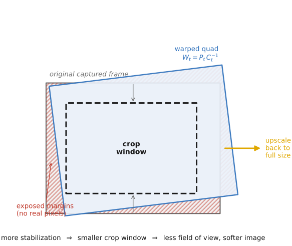
But the warp swings the frame quad off the original image grid, and that is where the borders go missing. Stabilizing means tilting and shifting each frame to sit on the smooth path; parts of the output rectangle then fall outside the pixels the camera actually captured, leaving empty margins along the edges that swung inward. There are two fixes, and the choice between them is the genuine tradeoff of the chapter:

• Crop and zoom (the standard route). Keep only a smaller central window that stays valid across all frames, then upscale it back to full resolution. The arithmetic is unforgiving: more stabilization means a smaller crop window means less field of view and a softer, upscaled image. This is the stabilization↔crop tradeoff. Typical consumer modes crop something like 10–20% of the frame to buy their steadiness (Figure 30.6.4⛶ fullscreen).
• Inpaint or fill from neighbors. Paint the missing borders using content from other frames (temporally nearby frames very likely saw those exact pixels a moment earlier or later), or hallucinate them with a generative inpainter (forward-ref Chapter 7.4, Generative AI and diffusion). This keeps the full field of view, at the cost of synthesized borders that may be wrong and a risk of flicker as the fill changes frame to frame.

A practical refinement softens the tradeoff: choose the crop margin adaptively, per clip or per segment, so that smooth shots crop almost nothing and only the violently shaky stretches pay the full field-of-view (FOV) cost. That turns a fixed global penalty into a content-aware one, the same spirit as adaptive everything else in this book.

30.6.5 Rolling-shutter correction: per-row pose and rectification🔗⧉

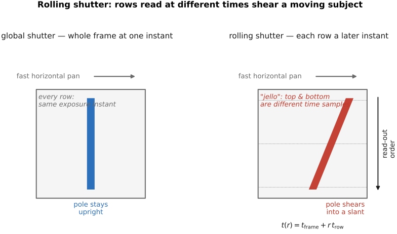
So far we treated each frame as a single snapshot taken at one instant. For most CMOS sensors that assumption is false, and the difference is visible. In a rolling-shutter CMOS sensor, exposure intervals are staggered by row. A global-shutter CMOS sensor instead exposes rows over a common interval, even if stored values are read out sequentially: the exposure reference time for row $r$ is

so the top of the frame and the bottom of the frame are captured a few milliseconds apart, sometimes up to roughly thirty. If the camera or the subject moves appreciably during that readout sweep, each row records a slightly different camera pose. The frame is no longer one time sample; it is a stack of them.

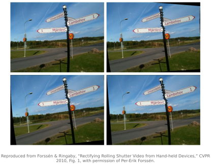
The artifacts are diagnostic because each one tells you what happened (Figure 30.6.5⛶ fullscreen). A horizontal pan skews vertical edges into slants, because each row was shot from a slightly panned-over viewpoint. A handheld tremor produces a wobble the community calls "jello," the image rippling as if seen through water. A spinning fan or propeller smears into impossible curved blades. All of it traces to the same cause: top and bottom of the frame are different time samples, which makes rolling-shutter distortion a time-axis sampling problem within a single frame (rows captured at different instants), a loose within-frame echo of the L16 sampling lesson rather than frequency-folding aliasing proper.

The model and the fix are the part spine again, now applied per row. For rotation-only correction, let $R(t)$ map world directions into camera coordinates at time $t$. Each scanline then has its own rotation. With calibration matrix $K$, a homogeneous image point maps by the homography below. To rectify, pick a single reference pose (the first row's, or the frame center's), and reproject every pixel from the pose at its row-time onto that common instant:

Each row gets warped by a slightly different transform; together the per-row warps "un-shear" the frame back to a single virtual instant, undoing the jello. It is correspondence-then-transport at the granularity of a scanline.

Everything now hinges on where the per-row pose comes from, and there are two answers. Karpenko et al. (2011) read $R(t)$ from the phone's gyroscope (after a one-time calibration of the gyro-to-frame timing and the row readout time $t_{\text{row}}$), which is robust, cheap, and (the thread from Stage 1) doubles as the rotation estimate for ordinary stabilization. Forssén and Ringaby (2010) instead estimate the per-row rotation from the image itself, fitting feature tracks to a continuous-time motion model and resampling against it. Accurate timing and calibration permit rotation-induced rolling-shutter correction. Translation requires scene depth, and independently moving objects require their own motion model. Finite-exposure blur also remains; resampling alone cannot undo it.

When rolling-shutter distortion is significant, rectify it before fitting a global path or model it jointly with stabilization, because otherwise the Stage-1 homography fits are corrupted by the very shear we are trying to remove: you would be estimating a camera path from frames that each lie about their own geometry. This is precisely the rolling-shutter caveat that the panorama chapter forward-references for continuous phone sweeps, where readout-time motion bites hardest because the phone is deliberately swinging the whole time (cross-ref Chapter 20.5, Continuous panoramas (e.g. on cell phones)).

Finally, the capture-side escape: a global-shutter sensor exposes all rows over the same interval and has no row-timing skew to correct. This is a sensor-design fix, paid for in sensor cost and complexity. It is the same engineering instinct that recurs throughout the book: when you can, build the system so you never have to invert the nasty artifact in the first place.