30.5 Hybrid low/high resolution and frame-rate imaging⧉
Camera spec sheets hide a simple limit. A sensor can clock out only so many pixels per second; that figure is set by the readout electronics, the bus, the analog-to-digital converters, and it is roughly fixed for a given chip. Spend that budget on spatial resolution and you get a gorgeous 50-megapixel still but a sluggish frame rate; spend it on temporal resolution and you get a thousand-frames-per-second high-speed camera that, frame for frame, is coarse and grainy. For a fixed readout mode and bandwidth, increasing the number of samples per frame limits frame rate. Faster electronics, parallel readout, bit-depth changes, cropping, and on-sensor storage can change that budget. This is the same flavor of impossibility as the exposure-versus-blur dial of Chapter 30.1, Motion blur, temporal sampling, and resampling: there the conflict was light against sharpness, here it is detail against speed. It has the same shape: a budget, and two things competing to spend it.
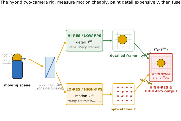
The trick of this chapter is to refuse the choice. Instead of asking one camera to be both, use two, with opposite settings, looking at the same scene: a high-resolution, low-frame-rate camera that supplies appearance: what the scene looks like in full detail, and a low-resolution, high-frame-rate camera that supplies motion: where everything went in the gaps between the detailed frames. Fuse the two and the output inherits the best of each: the detail of the slow stream, transported along the time line by the fast stream. The fast camera is cheap to run and cheap to read; the slow camera is expensive and rare. That division of labor (measure motion on the cheap channel, paint detail with the expensive one) recurs throughout the part, here implemented in hardware rather than software.
A single sensor forces a once-and-for-all bet on how to spend its pixels-per-second. Hybrid imaging refuses the bet by capturing two complementary streams at once, slow/detailed and fast/coarse, so that detail and motion are both recorded and the fusion is decided afterward, in software. This is L13.1 generalized from one camera's settings to a pair of cameras with opposite trade-offs: capture the full space–time set, then reconstruct whatever resolution-and-rate combination you want. It is the exact sibling of capturing a light field and choosing the aperture later, and of shooting a bracket and choosing the exposure later: the same move, on the joint space–time axis. (Registered in Big Lessons as L13.1, first appearing in the multiple-exposure material; this is a recurrence, now across two sensors.)
30.5.1 The space–time bandwidth trade-off⧉
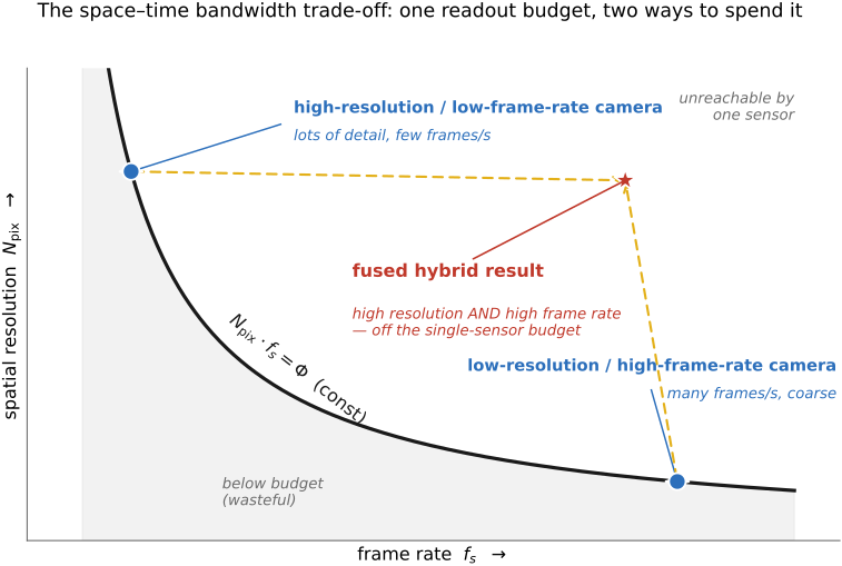
Write the constraint as an equation. A sensor's readout bandwidth (call it $\Phi$, in pixels per second) is roughly fixed, and it is split between the number of pixels per frame $N_{\text{pix}}$ and the frame rate $f_s$:
For a fixed throughput budget, the resolution/rate bound has a hyperbolic form: every point trades resolution for rate at constant product (Figure 30.5.1). A high-megapixel sensor sits far down the $f_s$ axis (lots of pixels, few frames); a high-speed sensor sits far down the $N_{\text{pix}}$ axis (many frames, few pixels). Available modes need not fill that curve: other hardware and exposure limits may reduce throughput further. The constraint is the channel between the photosites and memory, the same memory-bandwidth ceiling that limits any data-moving system (the hardware story told elsewhere in the book). It is an engineering resource constraint for the specified system, rather than a universal sampling limit shared by all cameras.
And as in Chapter 30.1, Motion blur, temporal sampling, and resampling, the two failure modes are the two ends of the curve. A slow/detailed camera can blur if its exposure is long. Low frame rate alone does not force a long exposure; short exposures at a low rate instead leave large temporal gaps. The fast/coarse camera resolves the motion crisply but cannot render fine texture. Each end has exactly what the other lacks. That complementarity is the whole opportunity.
30.5.2 The hybrid two-camera architecture⧉
The hardware is deliberately humble: two cameras that see the same thing, set to opposite ends of the curve. Sharing a view can be done two ways. A beam-splitter puts both sensors behind one lens, splitting the incoming light so the two streams are free of viewpoint parallax in an ideal common-pupil arrangement, though sensor scale, distortion, and alignment still need calibration, the cleanest registration, at the cost of light (each sensor gets a fraction) and bulk. Or the cameras sit side by side, cheaper and brighter but separated by a small baseline, so the two views must be registered by homography or by depth-aware warping before fusion (the parallax is small if the cameras are close and the scene is far). Either way the streams are brought into a common coordinate frame; from there it is all software.
A single sensor can also play both roles by reconfiguring itself per frame: alternate a full-resolution slow readout with binned or windowed high-speed readouts, or use a coded readout that captures a few high-resolution rows and many low-resolution ones. The phone variant of this is pixel binning: a quad-Bayer array reads $2\times2$ groups as one big, fast, low-noise pixel for video and as four separate pixels for a high-resolution still, the same hybrid trade hidden inside one chip.
30.5.3 Motion from the fast stream⧉
What does the fast, coarse stream actually contribute? Motion. Between two detailed but far-apart frames of the slow camera, the world moved, and a naive interpolation would have to guess how (the problem of Chapter 30.4, Frame interpolation and slow-motion synthesis). The fast camera records additional images that constrain motion between the sparse detailed frames; estimating motion from them is still an inference problem. Run Chapter 12.8, Optical flow on the high-frame-rate low-resolution channel and you get a dense per-frame displacement field $\mathbf{F}$ that says where every patch went at every fast instant; coarse in space. Upsampling must preserve motion boundaries; small objects and occlusions can disappear in the low-resolution stream. The flow links the sparse detailed frames.
Reconstruction is then transport, the part's spine once more. To synthesize a full-detail frame at any fast instant $t$, take the nearest detailed frame $I^{\text{HR}}$ at time $t_k$ and warp it along the motion the fast stream measured between $t_k$ and $t$:
where $\mathcal{W}$ is backward warping and resampling (from Chapter 11.1, Warping) and $\mathbf{F}_{t_k \to t}$ is the motion mapping composed across the fast frames. Compose trajectories at advected coordinates rather than simply adding vectors at one fixed pixel; backward resampling requires the corresponding inverse map on the target grid. Detail comes from $I^{\text{HR}}$; the trajectory it is dragged along comes from $I^{\text{LR}}$. Where the warp leaves holes (disocclusions the detailed frame never saw), the fast stream's own (coarse) pixels fill in, upsampled, until the next detailed frame refreshes the texture. The detailed frame provides appearance, and the fast stream provides continuous motion estimates.
30.5.4 Applications: deblur, space–time super-resolution, video from stills⧉
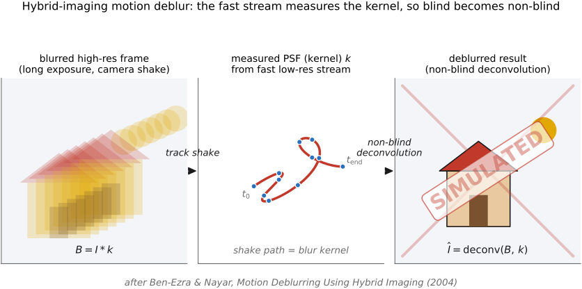
The first and cleanest use is motion deblurring. A long-exposure high-resolution frame caught during camera shake is blurred by a point-spread function $k$, the streak the shake traced, exactly the path kernel of Chapter 30.1, Motion blur, temporal sampling, and resampling. Deblurring it is deconvolution, $B = I * k$ inverted; the catch, the whole difficulty of Chapter 16.4, Blind deblurring, is that you do not know $k$. Hybrid imaging removes the blindness. Run the fast low-resolution camera during the same exposure and its frames record the camera's motion track directly: under a spatially invariant translational-blur approximation, that trajectory and the exposure weighting determine the PSF. Rotation, parallax, and object motion can require a spatially varying model. Estimating $k$ independently removes an important blind-deconvolution ambiguity. Non-blind inversion still needs regularization where the blur suppresses frequencies or noise is large. This is Ben-Ezra & Nayar's Motion Deblurring Using Hybrid Imaging Ben-Ezra & Nayar 2004: a hi-res/low-fps plus lo-res/high-fps rig in which the fast camera measures the blur kernel the slow camera suffers (Figure 30.5.3).
The second use is space–time super-resolution Shechtman, Caspi & Irani 2005. Take several low-resolution, low-frame-rate videos of the same event, each with slightly different sub-pixel and sub-frame offsets, and fuse them into a single video of higher resolution and higher frame rate than any input. It is the direct generalization of multi-frame Chapter 14.2, Multi-frame super-resolution (which combined sub-pixel-shifted stills into one sharper image) to the joint space–time grid: the sub-frame temporal offsets do for the time axis exactly what the sub-pixel spatial offsets do for the space axis, and the reconstruction recovers detail beyond the sampling limit of any one camera, with blur modeled as part of reconstruction. Deblurring is not free: exposure integration, conditioning, and noise limit recoverable temporal detail.
The third use enhances ordinary video with occasional high-resolution stills. Shoot a normal-resolution video and snap a few full-resolution photographs during it; then warp the detail of those rare stills onto every video frame, registered by flow, so the whole clip inherits the photographs' sharpness. This is Bhat et al.'s Using Photographs to Enhance Videos of a Static Scene Bhat et al. 2007, extended to dynamic content by Gupta et al. Gupta et al. 2009. It is the hybrid idea with the "fast low-res camera" being just the video itself and the "slow hi-res camera" being a sporadic shutter press, the same strategy of capturing detail occasionally and propagating it across the video.
30.5.5 Modern descendants⧉
The same principle appears in modern phones. Phone multi-camera systems can combine complementary measurements from wide, ultrawide, and tele modules. Their streams, frame rates, and use of learned fusion vary; the existence of a preview stream does not by itself imply this particular two-rate reconstruction. The same idea runs on the exposure axis instead of the resolution axis: Tocci et al.'s beam-split rig Tocci et al. 2011 splits light to sensors at different ISOs/exposures and fuses them into HDR video, the hybrid architecture pointed at dynamic range rather than detail, a close cousin of the bracket-and-merge logic of HDR merging.
The most extreme hybrid replaces the fast frame camera with an event sensor (Chapter 34.7, Event sensors): a chip whose pixels report brightness changes asynchronously, with fine timestamp resolution but finite latency, refractory time, and output bandwidth, but no absolute image. Pair it with a conventional sensor that provides occasional absolute frames and you have the hybrid taken to its limit: an asynchronous change stream supplying temporal evidence, and a slow absolute camera supplying appearance, the two reconstructed into sharp, deblurred, high-frame-rate video. (Direct velocity sensing, as in Chapter 34.6, Doppler / velocity imaging, is the same instinct of measuring motion at the sensor rather than inferring it from pixels.) Across all of these the recipe never changes: estimate motion from the fast channel, take appearance from the detailed channel, and fuse the two.
Recap: big lessons of this chapter
A single sensor forces a once-and-for-all bet on how to spend its pixels-per-second. Hybrid imaging refuses the bet by capturing two complementary streams at once, slow/detailed and fast/coarse, so that detail and motion are both recorded and the fusion is decided afterward, in software. This is L13.1 generalized from one camera's settings to a pair of cameras with opposite trade-offs: capture the full space–time set, then reconstruct whatever resolution-and-rate combination you want. It is the exact sibling of capturing a light field and choosing the aperture later, and of shooting a bracket and choosing the exposure later: the same move, on the joint space–time axis. (Registered in Big Lessons as L13.1, first appearing in the multiple-exposure material; this is a recurrence, now across two sensors.)