29.9 8-bit and fixed-point arithmetic🔗⧉

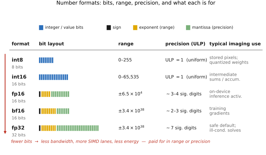
Replacing 32-bit storage with 8-bit storage quarters the bytes occupied by the affected samples. That can improve cache capacity and reduce traffic. It also reduces the set of representable values, and may require wider arithmetic, conversions, and scale handling. The resulting pipeline does not automatically run four times faster or produce the same image.

Choose precision stage by stage. A stored sensor value, a weighted sum, a color-transform output, and a neural activation have different ranges and error tolerances. Keep a higher-precision reference and test the complete output, including smooth gradients, deep shadows, saturated colors, and strong edges.

29.9.1 Integer versus fixed-point: where the binary point sits🔗⧉

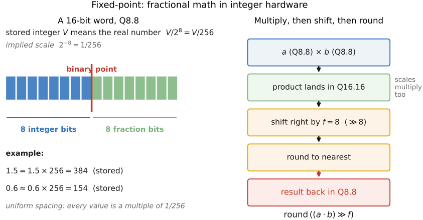
Unsigned 8-bit integers represent 0 through 255; signed int8 represents −128 through 127. Fixed-point attaches an implied scale to an integer. With $f$ fractional bits, stored integer $V$ represents

For this chapter, signed Q8.8 means a 16-bit two's-complement integer with eight fractional bits; the eight bits above the point include the sign. Its range is $[-128,127+255/256]$, with step $1/256$. Under this convention, 1.5 is stored as 384 and 0.6 rounds to 154. Other Q-notation conventions count the sign separately, so state total width, signedness, and fractional bits whenever ambiguity matters.

Add values directly only when their scales agree, using enough range for the sum. Multiplying two stored values $A,B$ with the same fractional-bit count produces a wide integer $P=AB$ with $2f$ fractional bits. To return to the original scale, compute

then apply any intended output saturation. Round before discarding the fractional bits; rounding an already shifted integer cannot restore them.

P = wide(A) * wide(B)
V = round_divide_by_power_of_two(P, f)  # specify the signed tie rule
output = clamp(V, output_min, output_max)

For nonnegative products and $f>0$, adding $2^{f-1}$ before an integer division by $2^f$ implements round-half-up. Signed values need an explicit rule; do not assume truncating division and a signed right shift round the same way. In Q8.8, $384\cdot154=59{,}136$ rounds back to 231, representing 0.90234375, close to the intended product 0.9.

Chapter 45.33, Photoshop 1.0, running shows the same principle in an early integer blur: preloading half a quantization step into a nonnegative accumulator performs rounding before the final shift. The exact error depends on quantized coefficients and boundary handling, so it should be measured rather than assigned one universal fraction of an output level.

Fixed-point spends its bits on a uniformly spaced grid. Floating point spends some of them on an exponent so that spacing grows with magnitude. If a stage has a known bounded range and needs roughly constant absolute precision, an exponent may buy little. If the range varies widely, the same fixed grid may waste codes near zero or overflow at the other end.

29.9.2 Rounding, dithering, and the banding trap🔗⧉

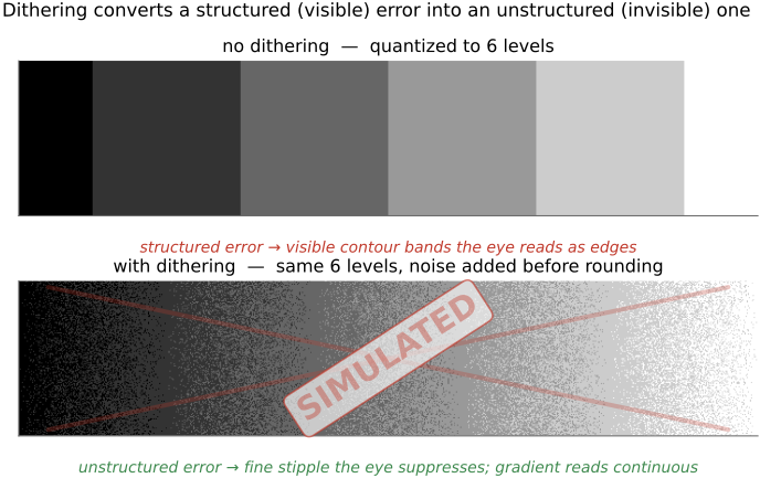
Dropping fractional bits creates a deterministic error. Flooring biases nonnegative values downward; truncation toward zero has a different signed behavior. Rounding to nearest limits the magnitude to half a step when no clipping occurs, but is not universally unbiased for every signal or tie rule.

A smooth gradient quantized to a coarse grid can reveal contour bands. Dither perturbs values before quantization so neighboring pixels need not cross a threshold together. It trades some visible structure for noise; it does not make the numerical error vanish or always make that noise invisible. Apply it where appropriate, often at final output quantization rather than at every internal stage. See Chapter 4.3, Encoding: linear, gamma or log for the role of encoding and viewing conditions.

For quantization step $\Delta$, the familiar variance $\Delta^2/12$ assumes a uniform error over one quantization interval. Undithered signal-dependent errors, clipping, and subsequent processing need not follow that model. As with the noise models in Chapter 2.8, Noise, signal-to-noise ratio and dynamic range, state the assumptions before propagating a variance.

29.9.3 Saturation and the width of the accumulator🔗⧉

Wrapping an over-range unsigned result into a small value can turn a bright highlight dark. Saturation avoids that at a bounded output by clamping to its representable interval. But clipping every intermediate is not physically required merely because a sensor saturates. Negative filter lobes and color transforms often need values below zero or above the final display range. Clip only where the specified algorithm or output format requires it.

Widen before adding or multiplying. For a weighted sum $S=\sum_{i=1}^{n}w_i x_i$, a conservative magnitude bound is

when $|x_i|\leq X_{\max}$. Include coefficient scaling and bias in the integer bound. A 7×7 sum of uint8 values can reach 12,495 and needs more than eight bits. A prefix sum over 12 million such samples can reach 3.06 billion and exceed signed 32-bit range. FP32 also cannot represent every large integer exactly, so replacing an integer accumulator with float does not automatically preserve counts.

The useful pattern is narrow storage, sufficiently wide accumulation, one defined rescaling, then output conversion. Repeated intermediate quantization can accumulate bias and noise. Coefficient quantization can also change a normalized filter's sum of weights; test constants to check its gain.

Storage width and accumulation width answer different questions. An input sample may fit in eight bits while the sum of a neighborhood does not. Widening only after the addition preserves an overflowed answer; the operands or accumulator must be wide during the sum. A weighted filter adds another scale: quantized coefficients and samples are multiplied before the result is shifted back to the chosen fixed-point representation. Work out the largest product and largest accumulated magnitude from those scales, then decide where rounding and saturation occur. Repeatedly narrowing inside the sum changes both the result and its error.

29.9.4 fp16 versus bf16: the exponent–mantissa bargain🔗⧉

Floating point uses a sign, exponent, and fraction field. IEEE binary16 (fp16) has 1 sign bit, 5 exponent bits, and 10 explicit fraction bits. Its largest finite value is 65,504, and the spacing near one is $2^{-10}$. BF16 has 1, 8, and 7 bits respectively, with spacing near one of $2^{-7}$. Its exponent range is similar to FP32's, while its precision is much coarser; their largest finite values are not identical.

Subnormal support and flushing behavior depend on the execution path. The Cloud TPU documentation, for example, describes BF16 multiplication with FP32 accumulation and flushing of BF16 subnormals in its documented implementation. Storage type alone does not specify accumulator precision or underflow behavior.

Both formats can be useful for training and inference. BF16's range can help avoid overflow; fp16 retains finer precision at comparable magnitudes. Neither prevents all instability. Mixed-precision execution can keep sensitive reductions, state, or master weights wider, and FP16 training may use loss scaling. Choose according to measured error and target support, not a rule that training must use one and inference the other.

Near 1, adjacent normal fp16 values are separated by about 0.00098, while adjacent bfloat16 values are separated by about 0.0078. The additional exponent bits of bfloat16 do not improve that local precision; they allow the binary point to move over a wider range. Conversely, a value of 100,000 exceeds fp16's finite range but is representable approximately in bfloat16.

Thus a stage storing small color differences near a large baseline and a stage carrying activations over many orders of magnitude can favor different formats. Wider accumulation can reduce some arithmetic errors but does not recover precision already lost when an activation was stored. Test the actual stage and hardware rather than assigning one format categorically to training and another to inference.

29.9.5 int8 quantization for neural inference🔗⧉

Affine quantization represents a real value with a scale $s>0$ and integer zero-point $z$:

The bounds are −128 and 127 for signed int8, or 0 and 255 for uint8. Real zero maps exactly to $z$ when it is a valid code; zero padding therefore uses $z$, not necessarily integer zero. Values beyond the chosen range clip. A wider calibrated range avoids some clipping but increases quantization steps.

For a dot product with input scale $s_x$ and weight scale $s_w$, accumulate corrected integer products:

The integer bias $b_q$ uses scale $s_xs_w$. For output scale $s_y$ and zero-point $z_y$, requantize as

An integer multiplier and shift can approximate the scale ratio. Use a sufficiently wide accumulator and intermediate product, and match the target's rounding convention. Jacob and colleagues derive this integer-inference approach Jacob et al. 2018; see their quantized-inference formulation.

Per-channel weight scales allow different output channels to use different ranges. Post-training calibration and quantization-aware training offer different ways to choose and adapt to the quantizer Gholami et al. 2021. Neither guarantees negligible error for a restoration network. Chapter 29.7, Efficient neural network inference discusses deployment and image-quality checks.

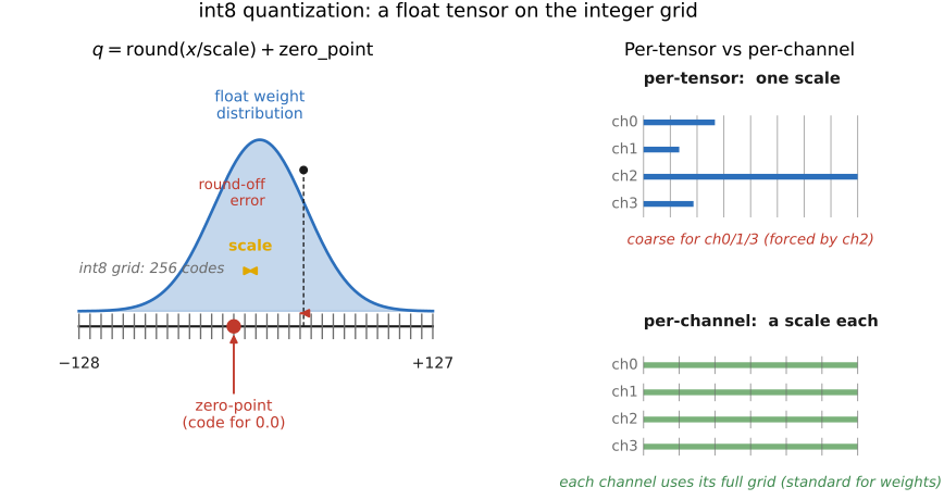
A single weight scale must accommodate the largest range among all output channels. A channel whose weights are much smaller then uses only a small fraction of the available integer codes. Per-channel scaling addresses that mismatch. Calibration estimates suitable ranges from representative inputs after training; quantization-aware training instead exposes the model to simulated quantization during optimization. The latter lets weights adapt to rounding and clipping, but requires training work. Both choices should be evaluated on difficult restoration inputs, where a small structured error may be visible even when an average metric changes little.

29.9.6 Where wider arithmetic matters🔗⧉

Use wider arithmetic where rounding is amplified: long accumulations, poorly conditioned systems, cancellation, or a large dynamic range. In a solve, check residuals and solution error; FP32 is not automatically sufficient. Mixed-precision solvers can use lower precision for some work and higher precision for corrections. Chapter 6.7, Image formation as a linear system explains the underlying sensitivity.

HDR data needs an encoding and precision that preserve the required radiance range. It need not always be FP32, but direct 8-bit linear storage is rarely adequate. In training, loss scaling and wider accumulation can address some range problems without changing every tensor to full precision.

Compare low-precision and reference outputs before final display clipping, then inspect the rendered result. Track overflow, underflow, saturation frequency, and systematic gain changes. Reducing bits is a useful optimization only after these errors and the actual runtime fit the application.