29.8 Automatic search for fast methods🔗⧉

Chapter 29.1, Algorithmic speedups exploits structure found by a designer. Automatic search explores combinations of such operations and learns their parameters. The designer still chooses the search space, constraints, losses, data, and execution model; those choices determine what the search can find.

Ma and colleagues' Searching for Fast Demosaicking Algorithms Ma et al. 2022 is a concrete example. It searches differentiable image-processing programs for a family of cost–quality tradeoffs. The task remains the reconstruction problem in Part 15, Demosaicking and joint methods; the contribution is a way to explore many candidate implementations. Chapter 15.4, Optimizing and searching classical demosaickers places it among the other ways of fitting classical demosaickers to data.

29.8.1 The problem is a curve, not a point🔗⧉

A preview and a high-quality still photograph can have different processing budgets. Instead of choosing one algorithm, retain candidates that offer different useful tradeoffs.

Let $C(p)$ be cost and $Q(p)$ quality for program $p$, with lower cost and higher quality preferred. Program $a$ dominates $b$ if

with at least one strict inequality. The nondominated candidates form a Pareto set. On a plot of cost increasing rightward and quality increasing upward, improvements point toward the upper left. A finite search returns the best known set among explored candidates, not proof of the globally optimal frontier or one program for every possible budget.

Suppose candidate A takes 5 ms and has lower reconstruction error than candidate B, which takes 8 ms. Under these two criteria, B is dominated and has no advantage. Candidate C takes 3 ms but has higher error than A: neither dominates the other. A preview with a tight frame budget may need C, while a saved photograph may afford A. Keeping both points gives the application a useful choice.

The frontier depends on the measured device, image sizes, quality criterion, and candidates considered. A program can belong to one measured frontier and disappear from another when memory or energy is added as a constraint. The search therefore produces evidence about a particular set of tradeoffs, not a universal ranking of algorithms.

29.8.2 What a broader search space can offer🔗⧉

Reducing a CNN's width or depth is a useful baseline. A richer search space can also choose task-specific operations, such as packing mosaic phases, local combinations, and separate green/chroma reconstruction. These operations encode useful demosaicking structure without requiring a dense layer everywhere.

A generic network can represent some of the same behavior, but expressing it efficiently is a different question. Compare search against well-tuned classical methods, small learned models, and relevant learned reconstruction baselines such as Gharbi et al. 2016. Do not assume that one family wins at every cost or on every camera.

29.8.3 Ma et al. 2022: searching structure and parameters together🔗⧉

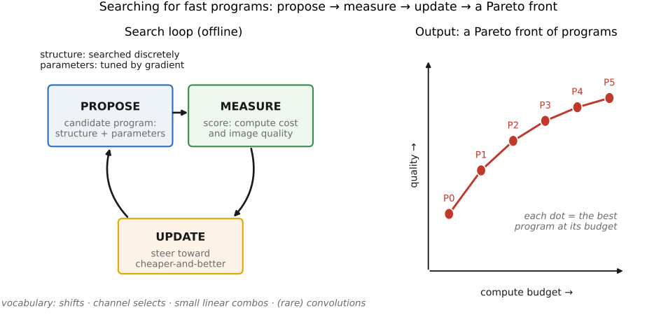
Ma and colleagues combine genetic mutations of program graphs with gradient-based fitting. Their domain-specific search separates green prediction from chroma prediction and includes conventional learned operations as well as imaging-specific building blocks. A cheap training procedure estimates quality during search; a weighted operation-count model estimates cost. Selected programs are then trained more fully and compiled to efficient Halide implementations for timing. These details are described in the paper.

The work includes Bayer and X-Trans demosaicking and joint demosaicking/super-resolution. X-Trans is periodic with a 6×6 pattern; adapting the search still requires representing that pattern and the task correctly. The result demonstrates reuse of the search framework, not removal of all domain-specific design.

A generic procedure captures the separation:

define legal program operations, shapes, cost limits, and data splits
initialize candidate programs
repeat until the search budget is spent:
    propose mutations of retained candidates
    reject invalid or over-budget graphs
    fit continuous parameters on training data
    evaluate quality on search-validation data and estimate cost
    retain candidates across useful cost ranges
retrain selected finalists with the declared training protocol
compile and benchmark them on the target device
freeze the selection, then evaluate on untouched test data

This is methodological pseudocode, not a reproduction of every detail of Ma et al.'s implementation.

The technical difficulty the paper solves is that the search ranges over two very different kinds of variable at once. The structure of a program, which operations exist and how they are wired into a graph, is discrete: you cannot take a derivative of "insert a shift here" or "delete this branch." The parameters that fill in a chosen structure, the linear coefficients, are continuous and differentiable. So this is a discrete–continuous optimization, and the two halves want different tools: combinatorial search over graphs for the structure, gradient descent for the parameters. Ma et al. interleave them, jointly solving for what the program is and what its numbers are, all while scoring each candidate on the two objectives, cost and quality, that define the Pareto front. The result is a program-synthesis procedure specialized to the specified demosaicking building blocks, training data, loss, and cost model.

29.8.4 Three axes of "search instead of design"🔗⧉

Three kinds of search appear in this book:

• Algorithm search varies the operations and their connections, usually trading output quality against cost Ma et al. 2022.
• Schedule search keeps the algorithm fixed while varying storage, recomputation, and parallel execution [@mullapudi-etal-2016; @adams-etal-2019].
• Optical co-design varies a physical encoding together with reconstruction, subject to manufacturing and capture constraints; see Chapter 33.7, End-to-end optimization.

29.8.5 The broader family, and what it costs🔗⧉

Program synthesis, superoptimization, and neural architecture search explore related spaces, but their correctness goals differ. Exact superoptimization may require equivalence to a specification. An approximate demosaicker is judged against data and a quality objective; a low reconstruction loss is not an equivalence proof.

Search has an offline cost that may be amortized across many deployments. It can also need repeating for a different target, input regime, or precision. A cost model that worked for one compiler and processor may misrank candidates elsewhere. Retest finalists on the actual device and record compilation settings, memory use, and sustained latency.

Quality estimates can be misleading too. Short training runs may favor quickly learned programs over better ones that converge slowly. Repeated search against a validation set can overfit it. Preserve final test data and inspect difficult images as described in Chapter 9.3, Image metrics and Chapter 9.2, The expert's eye as evaluation.

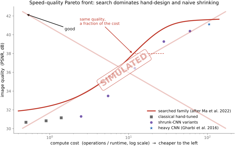
Algorithm search and schedule search can be composed. The first selects which operations represent the reconstruction; the second organizes their execution. A program with few arithmetic operations can still require poor memory access or excessive intermediates, so an operation-count frontier need not survive compilation unchanged. Timing compiled finalists tests the connection between the two searches. Searching the algorithm does not remove the performance-engineering problem; it supplies new candidates for it.

29.8.6 From search result to implementation🔗⧉

Deploy a searched program as you would any optimized implementation: freeze its graph and parameters, compile for the target, verify numerical behavior, and measure the complete path. The search objective identifies candidates; it does not replace the evaluation and deployment work.