29.7 Efficient neural network inference🔗⧉

A learned denoiser is a graph of tensor operations with weights, activations, and intermediate storage. Making it practical can involve changing the numerical format, the architecture, or how the runtime executes the graph. Some changes preserve the computation; others require retraining and change its output.

Define the budget in terms of the application: one-frame latency, sustained frames per second, memory, energy, and acceptable image quality. A viewfinder usually cannot amortize a large batch the way an offline service can. A model that fits as a weight file can still exceed memory limits through full-resolution activations and scratch buffers.

For a learned denoiser, changing float weights to a lower-precision representation preserves the network graph but changes its arithmetic. Removing channels changes both the graph and the shapes of its matrix operations. Distilling to a smaller network changes the mapping's parameterization and then trains it to reproduce useful behavior. These choices can have different effects even at the same operation count. A smaller irregular layer may use the hardware worse than a larger regular one, while an unsupported quantized operation may trigger an expensive fallback. Compare the complete deployed model on image quality, latency, and memory rather than inferring its speed from the number of weights alone.

29.7.1 Quantization: fewer bits per weight🔗⧉

Lower precision reduces storage for affected tensors and can enable faster arithmetic on supported backends. FP16, BF16, and integer quantization make different range and accuracy tradeoffs; Chapter 29.9, 8-bit and fixed-point arithmetic gives their numerical details. Weight-only compression does not imply integer execution for activations or accumulators.

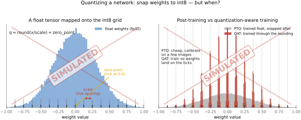
Post-training quantization calibrates an existing model using representative inputs. Include the actual preprocessing, exposure range, sensor noise, and image content encountered in deployment. A few bright, clean photographs will not characterize a night denoiser's activations. Measure clipping and reconstruction error on separate evaluation images.

The scalar map is the same one used in Chapter 29.9, 8-bit and fixed-point arithmetic: divide a value by its scale, round, add the zero point, and clip to the representable integer interval. Dequantization subtracts the zero point and multiplies by the scale. Applied to weights and activations, this replaces continuous values with points on a finite grid. A convolution then also needs an accumulation format and a rescaling step to map its output into the next tensor's quantization.

quantize(value, scale, zero_point):
    require scale > 0
    return clip(round(value / scale) + zero_point, integer_min, integer_max)

dequantize(code, scale, zero_point):
    return scale * (code - zero_point)

Suppose one output channel's weights span a much wider range than the others. A shared scale that accommodates its largest values leaves fewer useful codes for the smaller channels. Per-channel scales give each channel a more suitable spacing, when the backend supports them. Calibration faces the same tension with activations: a range wide enough for rare highlights can quantize ordinary values coarsely, while a narrower range can clip those highlights. This is an image-quality choice to measure, not a file-size change alone.

Quantization-aware training simulates the target quantization during training, using a surrogate gradient through rounding. It can improve robustness but does not guarantee recovery of the float model's quality. Per-channel weight scales help when channels have very different ranges; backend support constrains where such scales are allowed. Jacob and colleagues describe integer inference with simulated quantization Jacob et al. 2018, and Gholami and colleagues survey the design choices Gholami et al. 2021.

29.7.2 Pruning: fewer weights🔗⧉

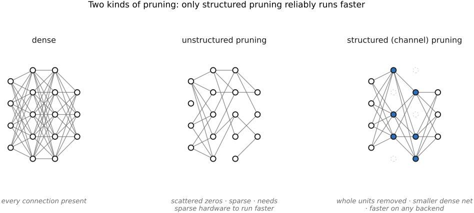
Pruning removes selected connections or units, often followed by fine-tuning Han et al. 2015 (learning weights and connections). Unstructured pruning creates scattered zeros. It reduces stored size only with a suitable sparse representation, and reduces execution time only when the implementation exploits that sparsity enough to offset indexing and scheduling overhead.

Structured pruning removes channels, filters, or other groups and yields smaller dense tensors. This is easier to use with dense kernels, but a smaller tensor can map poorly to hardware tile sizes or lose an optimized implementation. Measure the exported graph rather than predicting speed from parameter count.

The lottery-ticket experiments Frankle & Carbin 2019 (lottery ticket) found sparse subnetworks that trained successfully from particular initializations under their tested conditions. They do not establish that most weights in every imaging model are dispensable. Check texture, weak edges, and difficult capture conditions after pruning.

The lottery-ticket result also changes the interpretation of overparameterization. In the tested settings, the large network helped identify a smaller subnetwork together with an initialization from which it could train effectively. The value of the original capacity was therefore not only in the final dense set of weights. That is an explanation to investigate, not a promise that deleting small weights from any trained model recovers the same result.

29.7.3 Knowledge distillation: a small student, a big teacher🔗⧉

Distillation trains a student to reproduce useful behavior of a teacher Hinton, Vinyals & Dean 2015 (distillation). For classification, the teacher's probability distribution supplies information beyond the correct class label. For restoration, targets can be output images or intermediate features. The student can also retain a ground-truth reconstruction loss.

A simple image-output objective is

The student $S_\theta$ learns from the reference $y$ and teacher output $T(x)$, weighted by nonnegative $\alpha,\beta$. Choose the losses for the task. A teacher can transmit artifacts or hallucinated detail as well as useful behavior, so compare against training the same student without distillation.

A soft class distribution illustrates the extra information: two incorrect classes need not be equally implausible, and the teacher can express that ordering. For an image-output student, the teacher instead supplies a structured reconstruction or feature target across many pixels. The cost of running the large teacher is paid during training or target generation, while deployment runs only the student. The benefit must still be established against a student trained directly on the available references.

29.7.4 Low-rank and tensor factorization🔗⧉

A matrix $W\in\mathbb R^{m\times n}$ can be approximated by $UV$, with $U\in\mathbb R^{m\times r}$ and $V\in\mathbb R^{r\times n}$. Applying the factorization costs about $r(m+n)$ multiply-accumulates instead of $mn$, so arithmetic falls only when

The intermediate vector, extra dispatch, and memory traffic still have costs. A low-rank approximation of weights does not bound the final network's image error by itself; evaluate and usually fine-tune the modified model. Convolution-tensor factorizations make related tradeoffs, depending on which dimensions are factored.

This is the learned-weight version of approximating a filter by separable components. Instead of one wide matrix multiplication, apply one thin matrix and then another. The first produces a smaller intermediate representation; the second expands it to the output. Fewer arithmetic operations are useful only if the approximation is accurate enough and the implementation makes the intermediate inexpensive. A factorization can add an extra memory pass or a poorly supported kernel, so reduced parameter count and reduced measured latency are separate claims.

29.7.5 Efficient architectures: cheapness designed in🔗⧉

A standard $K\times K$ convolution with $C_{\mathrm{in}}$ input and $C_{\mathrm{out}}$ output channels uses approximately $K^2C_{\mathrm{in}}C_{\mathrm{out}}$ multiply-accumulates per output position. A depthwise convolution followed by a pointwise convolution uses

for a cost ratio $1/C_{\mathrm{out}}+1/K^2$, assuming depth multiplier one and matching spatial extents. MobileNets use this decomposition Howard et al. 2017 (MobileNets); see the original paper.

This architecture restricts the available spatial/channel mixing; it does not exactly factor an arbitrary trained dense convolution. Retraining can make it effective. Reduced arithmetic may also lower reuse enough that memory traffic dominates, limiting the latency gain.

EfficientNet explores coordinated scaling of depth, width, and resolution Tan & Le 2019 (EfficientNet). Such classification architectures offer useful building blocks, but their operating points are not automatically optimal for dense image reconstruction. A restoration network must retain fine spatial detail and often processes much larger activation maps.

For enhancement that can be represented by local color transforms, predicting a coarse coefficient field and applying it to the full-resolution image can avoid a large full-resolution network; see Chapter 29.1, Algorithmic speedups. That representation is insufficient for arbitrary geometric changes or texture synthesis.

The two operations divide the original job. The depthwise step applies one spatial filter to each input channel independently; it cannot mix information between channels. The pointwise step mixes channels at one location but has no spatial extent. This division is related to separability as an efficiency idea, though it separates channel mixing from spatial filtering rather than factoring a two-dimensional kernel into horizontal and vertical passes.

29.7.6 Neural architecture search: let the machine design it🔗⧉

Neural architecture search varies operations, connectivity, widths, and depth rather than only fitting weights Zoph & Le 2017 (neural architecture search). Hardware-aware search adds a target cost such as measured latency or a calibrated latency model. The search space and training procedure remain design choices.

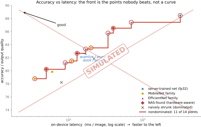
Measure finalists on the target and retest quality on data untouched by search. A model selected for one image size, batch size, precision, or backend may cease to be competitive when those change. Quantization, pruning, and distillation are optional tools to include or evaluate, not mandatory steps after every architecture search.

29.7.7 Hardware-aware deployment and the roofline🔗⧉

Inspect which operators execute on which device and which numerical formats they use. Convolution, bias, and activation can sometimes fuse without writing every intermediate. Layout conversions, unsupported operators, and CPU fallbacks can split that execution and erase a kernel-level improvement; see Chapter 29.6, Hardware backends: GPU, NPU, DSP.

Consider a convolution followed by bias addition and an activation. Three separate kernels can write the convolution result, read it to add the bias, write that result, and read it again for the activation. A fused kernel can apply the bias and activation while the convolution's output values are still local, then write the final tensor. The saved work is often intermediate traffic and launch overhead rather than fewer multiply-adds. It is the same producer-consumer reuse question as in Chapter 29.4, Halide programming, expressed in a neural-network graph.

Lower precision can reduce those bytes as well as changing arithmetic throughput, while fusion changes how often the bytes need to move. Their gains therefore depend on the current bottleneck and can overlap. A large matrix multiplication with substantial reuse may benefit from faster arithmetic; an operation moving a large tensor for little work may benefit more from avoiding an intermediate. Measure the actual tensor shapes and execution path before choosing between them.

The roofline in Chapter 29.2, Modern CPUs: memory hierarchy, parallelism, and what it takes to go fast helps relate operations to traffic Williams et al. 2009. Count bytes at the stated interface and use a consistent operation convention. A layer's name does not determine its bottleneck: tensor shape, batch size, implementation, and reuse matter.

Peak activation storage can dominate weights. Tiling inference reduces some memory demand but requires receptive-field overlap, discarding unreliable tile borders, and consistent padding. Global attention or whole-image normalization may prevent independent tiles from reproducing full-frame inference. Check seams and compare against a full-frame reference where possible.

29.7.8 Comparing deployable models🔗⧉

Compare candidates under the same deployment conditions. Report image quality and failures, one-frame latency, sustained throughput, peak memory, and the relevant energy budget. Prefer changes with a measured benefit on those quantities. A smaller weight file or a lower operation count is useful evidence about resource use, but it is not the final deployment result.