29.6 Hardware backends: GPU, NPU, DSP⧉
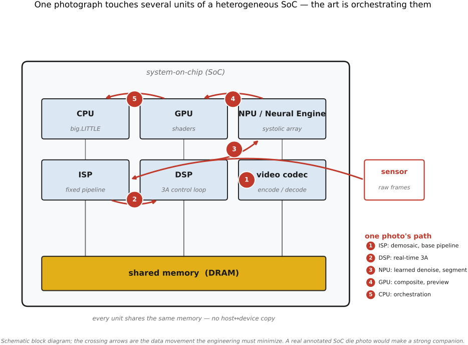
A camera can use several processors: an ISP for sensor-facing image stages, a CPU for control, a GPU for parallel image operations, and a neural accelerator or DSP for supported workloads. The assignment varies by device and software. A photograph does not follow one universal CPU–GPU–NPU sequence.
The useful question is where a stage runs efficiently in its surrounding pipeline. A CPU may finish a small filter sooner than an accelerator once dispatch and transfer costs are included. A slower kernel on the current device may beat a faster kernel elsewhere if moving the data costs more than it saves.
29.6.1 GPU: the data-parallel workhorse⧉
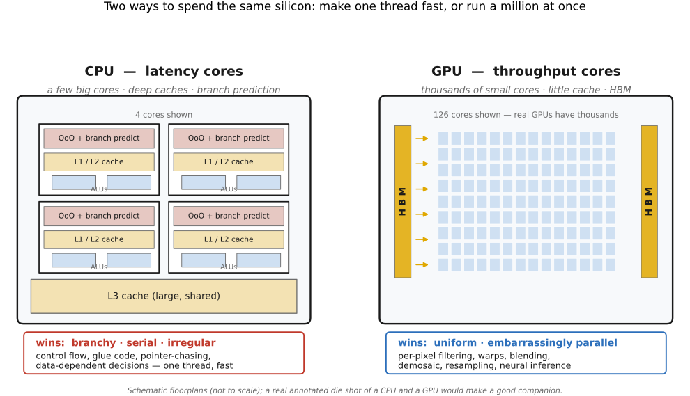
A GPU emphasizes throughput across many lightweight threads. It uses both memory hierarchy and concurrent execution: caches and local storage provide reuse, while ready groups of threads can execute when others wait. Neither mechanism guarantees that arithmetic units remain busy.
Many filters and warps have independent output pixels, even though those pixels read overlapping neighborhoods. Other stages, such as histograms and scans, have update dependencies that need a different decomposition. GPU performance depends on enough work, suitable memory access, and manageable synchronization.
SIMT groups threads for execution. NVIDIA calls a 32-thread group a warp; grouping and execution details differ across architectures. Coalescing combines nearby thread accesses into a small number of aligned memory transactions, not necessarily one transaction. Divergent control flow within a group can require execution of multiple paths with inactive lanes masked. Occupancy describes resident work relative to hardware capacity; more occupancy is useful only when it helps the workload, and can conflict with register use or tile storage. The CUDA best-practices guide gives the NVIDIA-specific details.
Programmer-managed shared memory can retain a tile for cooperative reuse. Loading it costs instructions and often synchronization, so use it when the reuse pays for those costs. A simple streaming kernel may work well through ordinary cached memory.
CUDA, Metal, OpenCL, and Vulkan compute provide different programming and deployment paths. Halide can target supported backends with an appropriate schedule and toolchain; availability and operator support must be checked for the actual release and device.
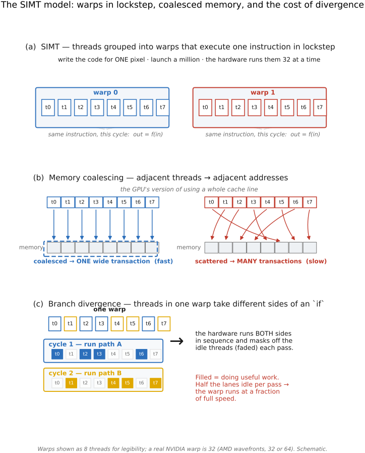
if, the hardware runs both sides and masks the idle threads, so the warp runs at a fraction of full speed. Locality and parallelism, with the knobs renamed. (Schematic.)For a discrete GPU, account for host-device copies and synchronization. On an integrated GPU, shared physical memory can avoid some copies, but layout conversion, cache coherence, bandwidth contention, and ownership transitions still cost time. Keep useful work on the device across several stages where possible.
Consider neighboring GPU threads processing neighboring output pixels. If they read neighboring input samples, their requests can use a small set of memory transactions. If each thread follows a scattered index, the same number of useful samples can require more transactions. Loading a tile into a programmer-managed shared buffer can make neighborhood reuse explicit, but the buffer consumes resources that could otherwise support more resident work. A larger tile can therefore improve reuse while reducing occupancy. Measure the combined effect rather than optimizing either quantity in isolation.
29.6.2 The neural accelerator: NPU and TPU⧉
Neural accelerators specialize in tensor operations and their data reuse. A systolic array, such as the TPU architecture described by Jouppi and colleagues Jouppi et al. 2017, passes operands through multiply-accumulate units to reuse them efficiently. Other accelerators use different organizations; “NPU” does not imply one particular internal design. Google's Tensor is a system-on-chip family name, not a synonym for one neural execution unit.
Supported convolutions or matrix operations can run efficiently at low precision. The practical limits are operator coverage, tensor shapes, layout, precision, local storage, and compiler mapping. A network with unsupported operations can split into several subgraphs with transfers or CPU fallbacks between them.
Check the compiled graph and measure end-to-end execution. Reducing precision or fusing operators helps only if the target implements the resulting operations efficiently and image quality remains acceptable. Chapter 29.7, Efficient neural network inference and Chapter 29.9, 8-bit and fixed-point arithmetic develop these choices.
The systolic array in the TPU example illustrates how data reuse can be built into the hardware Jouppi et al. 2017. Matrix multiplication repeatedly multiplies each element by elements along another row or column. Passing operands through a grid of multiply-accumulate units lets neighboring units reuse them while partial sums accumulate locally. Fetching each operand anew from external memory for every multiplication would waste much of the potential throughput.
This is one accelerator design, not a description of every NPU. Its advantage depends on filling the array and expressing the workload in supported operations and precisions. Small matrices, irregular work, or unsupported stages can leave units idle or require transfers to another processor. The useful question for an imaging pipeline is how much of the whole computation can stay on the accelerator, including its intermediate data.
29.6.3 DSP: the real-time control loop⧉
Digital signal processors support repeated signal operations through combinations of efficient multiply-accumulate instructions, vector units, local memory, and execution mechanisms suited to streaming work. Depending on the system, a DSP may run image kernels, neural workloads, or parts of camera control.
Auto-exposure, autofocus, and auto white balance have latency and stability requirements, but they do not universally run on a DSP or update all settings before every next frame. The controller may use delayed statistics and run across several camera subsystems. For deadline-sensitive work, measure worst relevant latency and jitter as well as average throughput; see Chapter 8.10, Auto-exposure and auto white balance.
29.6.4 ISP, FPGA, and ASIC: the fixed-function end⧉
An ISP combines dedicated image-processing blocks with configuration and, in some designs, programmable components. Sensor correction, demosaicking, denoising, color, and tone operations can stream through line buffers at high efficiency. Its parameters and supported modes can change even when the hardware datapath cannot implement an arbitrary new algorithm. Part 8, Basic image processing and ISP describes the operations independently of this hardware assignment.
An FPGA implements reconfigurable logic and routing, allowing a custom datapath to be changed after manufacture. An ASIC is a chip designed for an application; it can contain fixed-function blocks, programmable cores, or both. An ISP or neural accelerator can itself be part of an ASIC, so these names are not mutually exclusive positions on one ladder.
Specialization can improve energy and area efficiency for a matched workload, at a cost in design effort and flexibility. Volume, latency requirements, available interfaces, and expected algorithm changes determine whether it is justified.
29.6.5 The heterogeneous SoC, and the spectrum to carry away⧉
A system-on-chip connects several processing blocks and memory interfaces. Shared memory makes cooperation easier, but it remains a resource that the blocks compete for. An implementation must coordinate buffer ownership, layout, synchronization, and execution order.
For a serial path, a useful accounting is
Measure these contributions without double-counting overlap. With pipelining, frame throughput is governed by the bottleneck resource and dependencies, while one frame's latency follows its critical path. Higher throughput can coexist with higher latency if batching or queueing is introduced.
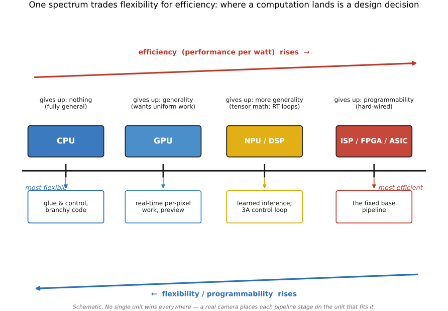
Choose the unit that executes the required operations efficiently within the whole pipeline. Include movement and conversion costs. Flexibility and efficiency trade off, but CPU, GPU, DSP, NPU, and ISP do not have a universal ordering of performance per watt.
29.6.6 On-device ML runtimes, and why the work stays on the phone⧉
A deployment runtime maps supported parts of a trained model to available implementations. LiteRT provides accelerator integration; ONNX Runtime uses execution providers; Core ML exposes allowed compute-unit configurations. These are not a universal fallback order of NPU, then GPU, then CPU. Selection depends on runtime settings, backend support, model operations, shapes, and device. Consult LiteRT, ONNX Runtime execution providers, and Core ML compute units.
Inspect placement and conversion overhead after compilation. A model that loads successfully may still execute expensive parts on the CPU. Repeated boundaries between accelerators can outweigh the savings from individual accelerated layers.
Keeping processing local avoids network upload latency, supports offline use, and reduces exposure of image data to remote services. It does not by itself guarantee privacy; storage and application behavior still matter. Cloud processing remains useful for workloads that exceed local resources. HDR+ is a documented example of on-device burst processing Hasinoff et al. 2016, not evidence that all computational photography must remain on the phone.
Recap: big lessons of this chapter
Choose the unit that executes the required operations efficiently within the whole pipeline. Include movement and conversion costs. Flexibility and efficiency trade off, but CPU, GPU, DSP, NPU, and ISP do not have a universal ordering of performance per watt.