29.4 Halide programming⧉
We will build a three-tap horizontal blur followed by a three-tap vertical blur, then change its execution schedule. The definitions stay readable while we vary intermediate storage, vectorization, and threading. Chapter 29.3, Halide at a high level: decoupling algorithms from schedules explains the motivation; here the choices become code.
The examples use Halide's C++ interface and the scheduling model in the official tutorials and lecture slides Ragan-Kelley et al. 2018 (CACM). Python exposes the same core constructs with hl.Func, hl.Var, and square-bracket indexing. In C++, include Halide.h and link against the Halide library. In Python, import the bindings as import halide as hl. A C++ definition such as f(x, y) = expression becomes f[x, y] = expression; expression operations use names such as hl.min, hl.max, and hl.cast. Many scheduling calls have the same names in both interfaces, though signatures and supported features should be checked against the installed release.
Choose the host interface to fit the surrounding application. Python makes it convenient to inspect arrays and experiment interactively; C++ integrates directly with a C++ application. This choice concerns the program that constructs and invokes the pipeline. In either case, Halide compiles the pixel computation rather than executing a host-language loop once per pixel. Ahead-of-time compilation separates pipeline generation from the application that ultimately calls the generated function.
Halide constructs regular array computations. The host handles I/O, application state, and control such as an iterative solver's convergence test. Reduction domains can have extents supplied at runtime, but they describe bounded iterations rather than an arbitrary data-dependent while loop.
29.4.1 Getting started with Halide⧉
Halide is a compiler library embedded in a host program. The host constructs the pipeline, requests compilation, and invokes generated code. A Func definition builds an expression graph; it does not yet process pixels.
Consider blur_x(x,y) = (bounded(x-1,y) + bounded(x,y) + bounded(x+1,y))/3.0f. The host executes this C++ statement, but none of the input pixels is read yet. The overloaded + and / operators construct nodes describing additions and a division. Calls to bounded become references to another stage. The result is a tree describing how to compute one output value, connected to the definitions of the stages it uses (Figure 29.4.2).
This is metaprogramming: we run a program whose output is another program. C++ parses the expression and calls the overloaded operators; Halide receives the resulting data structure. A schedule then specifies how to turn that description into loops. realize requests compilation when needed and executes the generated code over a particular output region.
The distinction allows ordinary host code to build a pipeline. A C++ loop can construct ten successive blur stages, for example. That loop runs while constructing the graph, producing ten Func definitions. The image-processing loops run later, after Halide has compiled that graph. Similarly, a host if can choose which algorithm to construct without introducing a conditional at every output pixel. The host language provides its existing abstractions, libraries, and control flow, while Halide retains a representation it can analyze and schedule.
This complete C++ example uses a synthetic one-channel image so that file I/O and color management do not obscure the scheduling example. Input and output have zero coordinate minima, and the values are floats.
#include <Halide.h>
#include <cstdio>
using namespace Halide;

int main() {
    Buffer<float> input(17, 13);
    for (int yy = 0; yy < input.height(); ++yy)
        for (int xx = 0; xx < input.width(); ++xx)
            input(xx, yy) = float(xx + 2 * yy);

    Var x("x"), y("y");
    Func bounded = BoundaryConditions::repeat_edge(input);
    Func blur_x("blur_x"), blur_y("blur_y");
    blur_x(x, y) = (bounded(x-1, y) + bounded(x, y)
                    + bounded(x+1, y)) / 3.0f;
    blur_y(x, y) = (blur_x(x, y-1) + blur_x(x, y)
                    + blur_x(x, y+1)) / 3.0f;

    // Insert one candidate schedule here, before realize.
    Buffer<float> output = blur_y.realize({input.width(), input.height()});
    std::printf("center: %g\n", double(output(8, 6)));
    return 0;
}
The center should be 20: a normalized symmetric blur preserves this affine ramp away from boundaries. Also test a constant, an impulse, and corners against a small reference loop. The deliberately odd image dimensions will exercise schedule tails later.
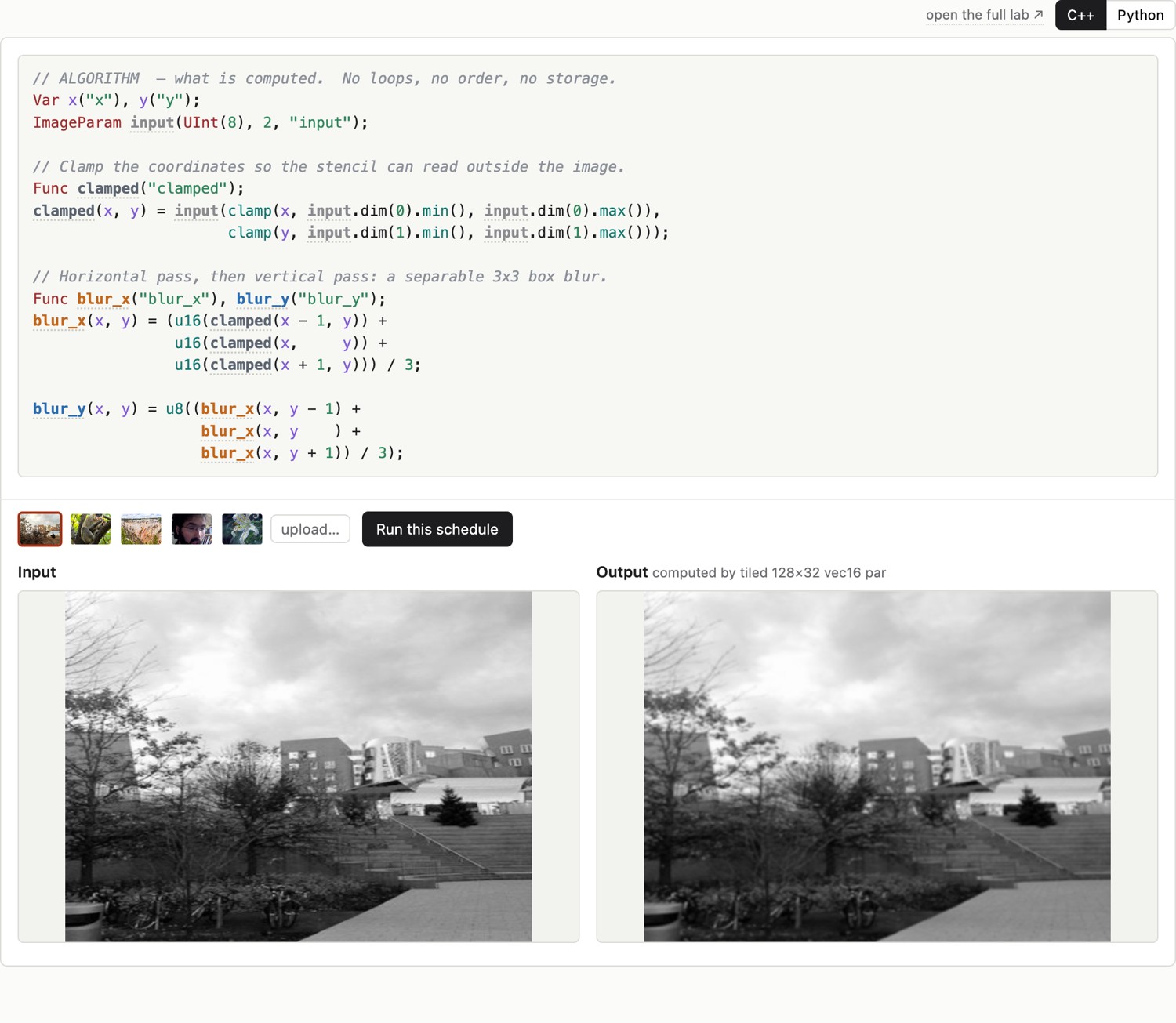
load_image and save_image in C++, hl.load_image and hl.save_image in Python); everything between them is Halide.realize compiles just in time when needed and computes a requested region. Ahead-of-time compilation instead produces code and an interface that the application links with the required Halide runtime support. The application need not ship the Halide compiler. Compilation time and execution time are separate costs.
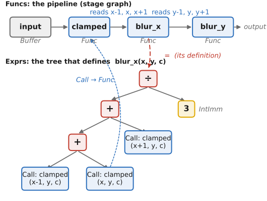
Funcs and Exprs, with no pixel yet computed. Top, the pipeline of stages, input → clamped → blur_x → blur_y, each arrow a data dependence. Bottom, the Expr tree that is the definition of blur_x: the overloaded +, +, and / have assembled (clamped(x-1,y,c) + clamped(x,y,c) + clamped(x+1,y,c)) / 3 as an abstract syntax tree over a division by the integer 3. Its three leaves are Call nodes pointing back into the clamped Func, so the whole pipeline is one connected graph, and realize is what walks it, schedules it, and compiles it.Func is a handleA Func refers to a definition, update definitions if any, and scheduling information. A simplified model of the stored information is:
// Explanatory data model, not Halide's internal class declaration.
struct StageDescription {
    std::string name;
    std::vector<Var> arguments;
    std::vector<Expr> values;
    // Update definitions and scheduling information are stored as well.
};
Each Expr refers to an expression node: an arithmetic operation, a constant, a variable, or a call to another stage. Nodes retain their operands, forming the graph that the compiler traverses.
In f(x,y) = expression, calling f(x,y) returns a FuncRef, a proxy referring to this function at these arguments. Assignment to that proxy installs a definition. By contrast, Func a = b copies a handle and makes an alias; it does not clone the pipeline. Changing the schedule through a therefore changes the same underlying function named by b. To compare independently modified schedules, construct a fresh pipeline for each candidate.
Just-in-time and ahead-of-time compilation serve different workflows. realize compiled the pipeline just-in-time: it ran Halide's compiler inside your process, generated the machine code, and executed it, in one call. That is the fastest way to a result, so learn and prototype with .realize. Shipping is different. There you compile ahead-of-time: a small generator program compiles the pipeline once into an object file and a header, which you link into an application that need not ship the Halide compiler. The generated code still needs its runtime support and any required target libraries. Ahead-of-time compilation is useful when deployment needs a precompiled kernel and a predictable startup path. The rule of thumb: .realize while you learn, a generator when you ship.
29.4.2 Functional, with no loops: Func, Var, Expr⧉
A Halide pipeline is a graph of functions. A pure stage describes its value at an arbitrary integer coordinate in terms of the input and earlier stages. For example, the horizontal blur says what one blurred pixel is, without specifying which row should be computed first or where the intermediate image should live. Those decisions can therefore be made by the schedule. An imperative loop that overwrites an array may make its traversal order part of the answer; the pure definition keeps the value separate from that traversal. Update definitions, including reductions, require additional dependence analysis.
You write the formula for an output pixel. Four types distinguish the formula from the pixels it will eventually produce:
- A
Varnames an integer coordinate, usuallyx,y, orc. It is a symbolic coordinate, not a C++ counter being incremented through the image. Defining a stage at(x, y)describes an arbitrary requested pixel. - An
Expris a formula such asx + yorinput(x, y) * 2. It is a recipe for a value. Overloaded operators construct expression nodes while the host program runs; they do not traverse the image and apply the operation to its samples. - A
Funcnames a stage and holds its definition. It is a rule for computing pixels, not an allocated image. Calling oneFuncin another's definition records a dependency. Whether that dependency becomes a stored intermediate or an expression evaluated at each use is a scheduling decision. - A
Buffercontains the actual samples in memory, with minima, extents, and strides. The examples use the first coordinate forx, unlike the row-first convention of many array libraries. A coordinate convention does not imply a particular memory layout; the strides specify that layout.
The smallest example makes a gradient: the value at each pixel is the sum of its coordinates.
Var x("x"), y("y");
Func gradient("gradient");
gradient(x, y) = x + y;
Buffer<int32_t> ramp = gradient.realize({8, 6});
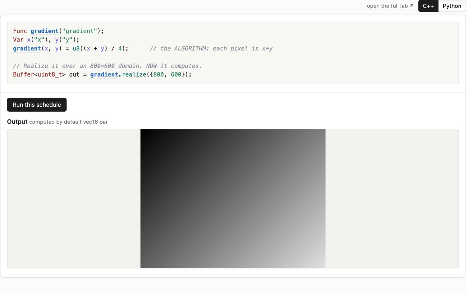
gradient(x, y) = x + y is a Func with no input at all: its value depends only on where it is. Nothing computes until realize names a rectangle, and then the whole image appears at once.Read the gradient program in two phases. The declarations and assignment run in the host C++ program and build the description of gradient. At that point there is no 8×6 ramp in memory. realize({8, 6}) requests that rectangle, compiles the pipeline as needed, and executes the generated loops to fill a buffer. Pixel (3, 2) becomes 5. A different schedule can visit that pixel earlier or later without changing its formula.
This distinction is also why a C++ loop around a definition does something different from a pixel loop. A host loop can build ten successive blur stages, leaving ten nodes in the pipeline graph. The schedule then decides how the pixels of those stages are evaluated. This use of a program to construct another program is metaprogramming, and it lets ordinary C++ functions and loops generate a complicated pipeline without writing a parser for a separate language.
A convolution contains two kinds of loops. The outer loops visit output pixels. The inner loops add the input contributions needed for one output pixel:
for y in output_rows:
    for x in output_columns:
        total = 0
        for ky in kernel_rows:
            for kx in kernel_columns:
                total += kernel(kx,ky) * bounded(x-kx,y-ky)
        output(x,y) = total
Halide leaves the output loops implicit: a definition describes an arbitrary requested pixel. The sum remains part of that definition, expressed through a reduction domain or a fixed expression. Removing explicit output loops allows the schedule to choose their order and grouping; it does not remove the arithmetic required by the neighborhood. The reduction section below shows how to express the inner sum.
Every intermediate has output pixels of its own. The implicit loops for blur_x visit the domain needed by its consumers, which may include a halo beyond the requested blur_y rectangle. The input sum inside one output formula remains part of the algorithm. For a fixed three-tap filter we can spell out its three terms; for a general kernel, a reduction domain describes the terms to accumulate. The schedule cannot drop that sum simply because the output traversal was left implicit.
Use Halide expression functions for runtime choices. A host C++ if decides what graph to build; Halide select chooses between values in that graph. Do not use select as a short-circuit guard for an invalid load or division: both value expressions may be evaluated. Make accesses and denominators safe before selecting. Pure stages permit broad scheduling freedom; update definitions introduce additional constraints.
29.4.3 A first image pipeline: brighten, then blur⧉
For unsigned 8-bit input, widen before arithmetic and define the output conversion explicitly. This fragment assumes an existing zero-origin two-dimensional Buffer<uint8_t> input8:
Var x("x"), y("y");
Func bright("bright");
Expr value = cast<float>(input8(x, y)) * 1.5f;
bright(x, y) = cast<uint8_t>(clamp(value + 0.5f, 0.0f, 255.0f));
It rounds nonnegative values to the nearest integer with half values upward, then saturates. If the input is display-encoded, this scales code values; it is not a scene-linear exposure adjustment. Choose the domain according to Chapter 8.3, Tone point operations. Halide's promotion rules differ from C's: adding narrow integer expressions does not automatically widen them. See the type-system tutorial.
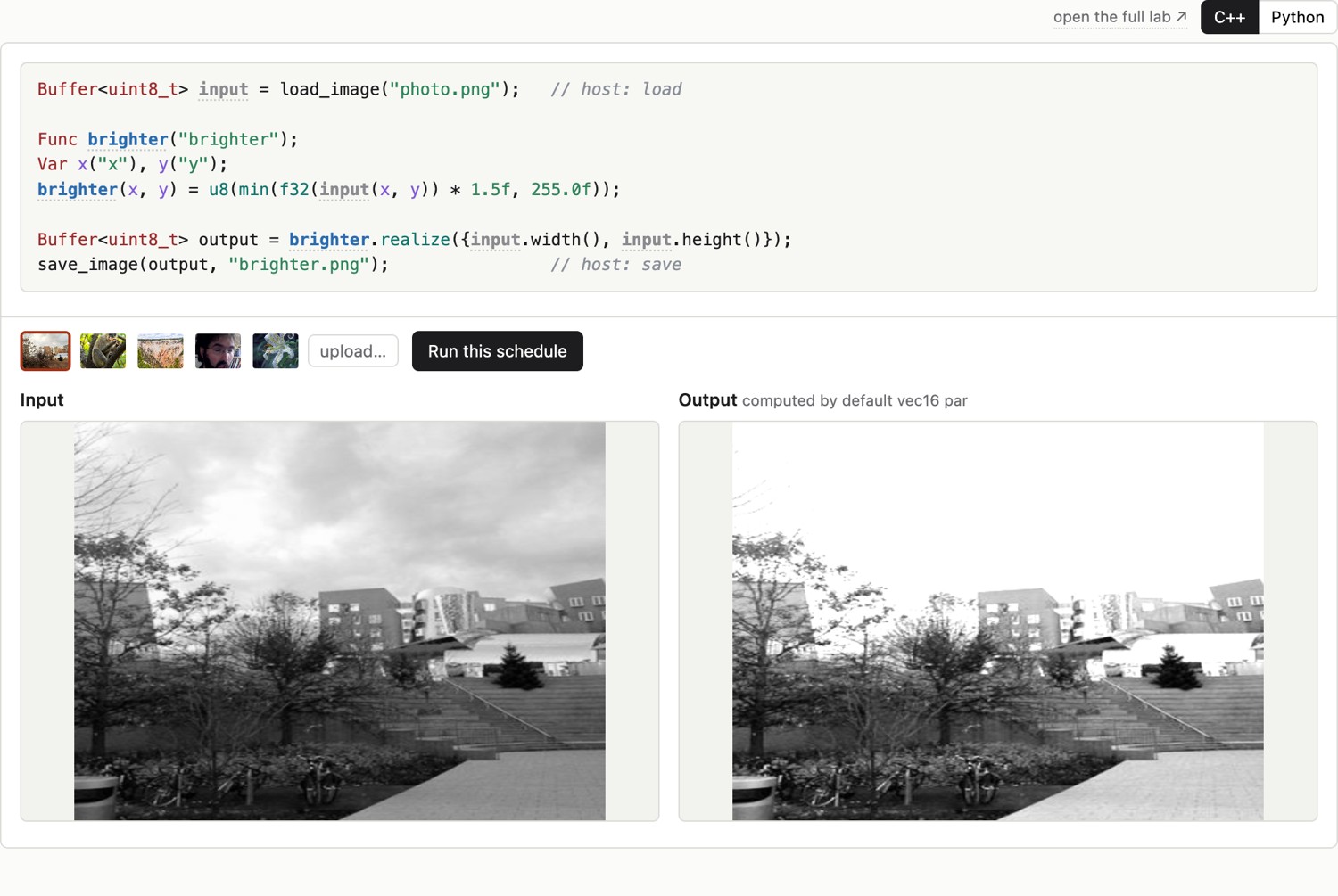
The float blur defined earlier avoids intermediate integer rounding. For color, add a channel coordinate and preserve the actual layout; do not assume the channel axis is contiguous merely because it is named c.
blur_x feeding blur_y, each defined by the value of one output pixel.Each vertical output row needs three rows of the horizontal producer. Adjacent output rows share two of those producer rows. The schedule determines whether they reuse stored results or recompute them.
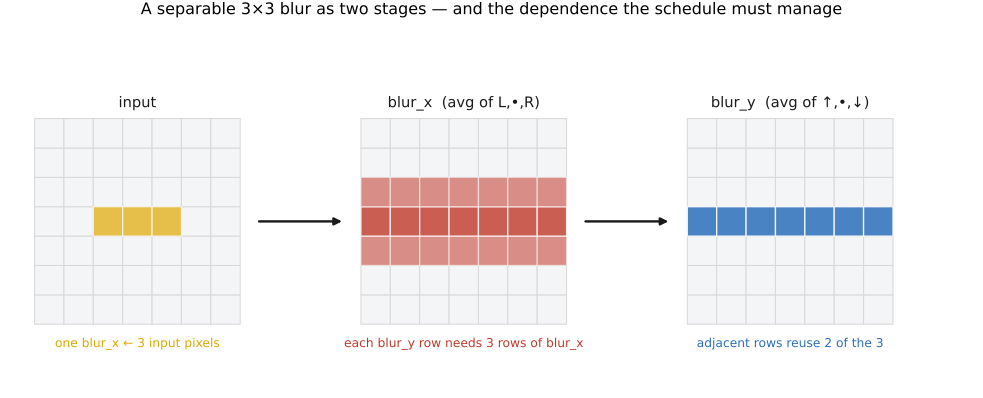
blur_x (the producer) averages each pixel with its left and right neighbors; blur_y (the consumer) averages the result with its top and bottom neighbors. The dependence that drives every scheduling choice: each output row of blur_y reads three rows of blur_x, and adjacent output rows overlap in two of those three, so how much of blur_x to compute, store, or recompute per row of blur_y is exactly the trade the schedule makes.29.4.4 Reductions: RDom, sums, and histograms⧉
A reduction has an initial definition and one or more updates. For a 7×7 box over the float bounded function:
Func sum7("sum7"), box7("box7");
RDom r(-3, 7, -3, 7, "r");
sum7(x, y) = 0.0f;
sum7(x, y) += bounded(x + r.x, y + r.y);
box7(x, y) = sum7(x, y) / 49.0f;
RDom takes a minimum and an extent for each dimension. Here both offsets range from −3 through 3. This is a direct 49-tap reduction; a separable implementation uses two seven-tap reductions.
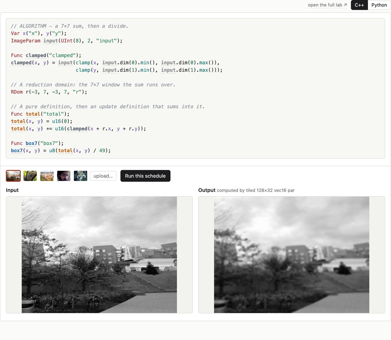
RDom over the window, a pure definition that zeroes the accumulator, an update definition that sums into it, and a divide. Run it and the 49-tap average appears below the listing.For a histogram, updates choose their destination from the data. With a nonempty zero-origin 8-bit input buffer:
Var bin("bin");
Func histogram("histogram");
RDom pixels(0, input8.width(), 0, input8.height(), "pixels");
histogram(bin) = cast<int64_t>(0);
histogram(cast<int32_t>(input8(pixels.x, pixels.y))) += cast<int64_t>(1);
The wide accumulator makes the counting range explicit. An ordinary parallel loop over input pixels would race when several pixels increment the same bin. Partial histograms followed by a merge, or supported atomic updates, can provide a correct parallel implementation.
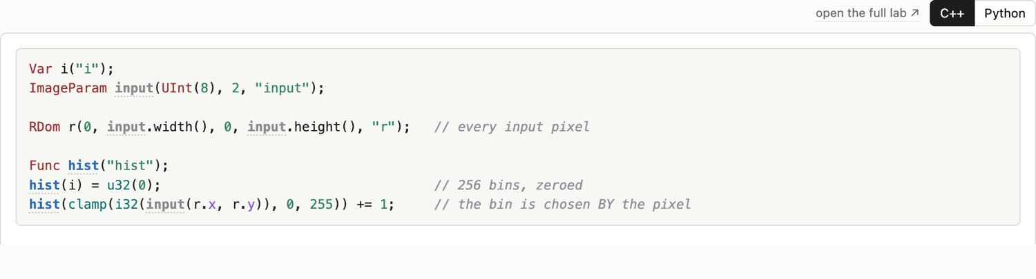
rfactor). Code only here, since 256 bins are not a picture.Not all updates are associative. A prefix scan depends on earlier values, while floating-point sums change rounding when regrouped. The pure initialization and each update have their own schedules; optimizing one does not automatically optimize the others. The update-definition tutorial develops these restrictions.
29.4.5 The two extremes: root and inline⧉
Construct a fresh copy of the blur for each candidate schedule. Start with the consumer's loops, then decide where its producer runs.
blur_x.compute_root();
This computes the required horizontal region before the output. For a zero-origin $W\times H$ output and the centered vertical stencil, that region has width $W$ and rows from −1 through $H$. Stored values are reused by neighboring output rows. Whether the full intermediate reaches DRAM depends on size and cache behavior.
allocate horizontal storage for [0,W) × [-1,H+1)
for y in [-1,H+1):
    for x in [0,W): compute horizontal(x,y)
for y in [0,H):
    for x in [0,W): compute output(x,y) from three horizontal rows
Alternatively, leave the pure producer at its default inline schedule:
blur_x.compute_inline();
Its expression is substituted at each use, eliminating a producer buffer. The vertical stencil then contains three horizontal sums. This can repeat arithmetic, though compiler simplification and cache reuse determine the final instruction and traffic counts. Inlining is often appropriate for cheap pointwise stages. Functions with updates cannot generally be treated as freely inlineable pure expressions.
Neither root nor inline is inherently a bad schedule. An expensive shared producer may belong at root; a cheap expression may belong inline. Compare them before adding complexity.
Use blur_y.print_loop_nest() to inspect the resulting organization. Trace small runs with trace_stores() or expression-level prints when needed, and turn tracing off for benchmarks.
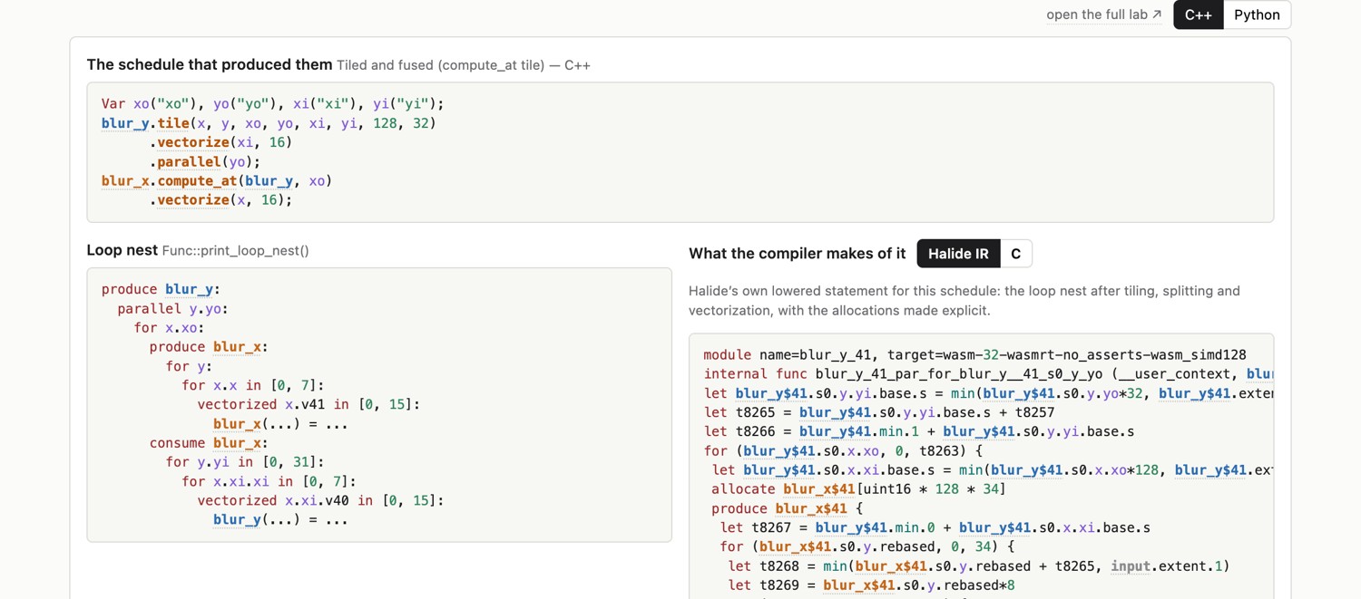
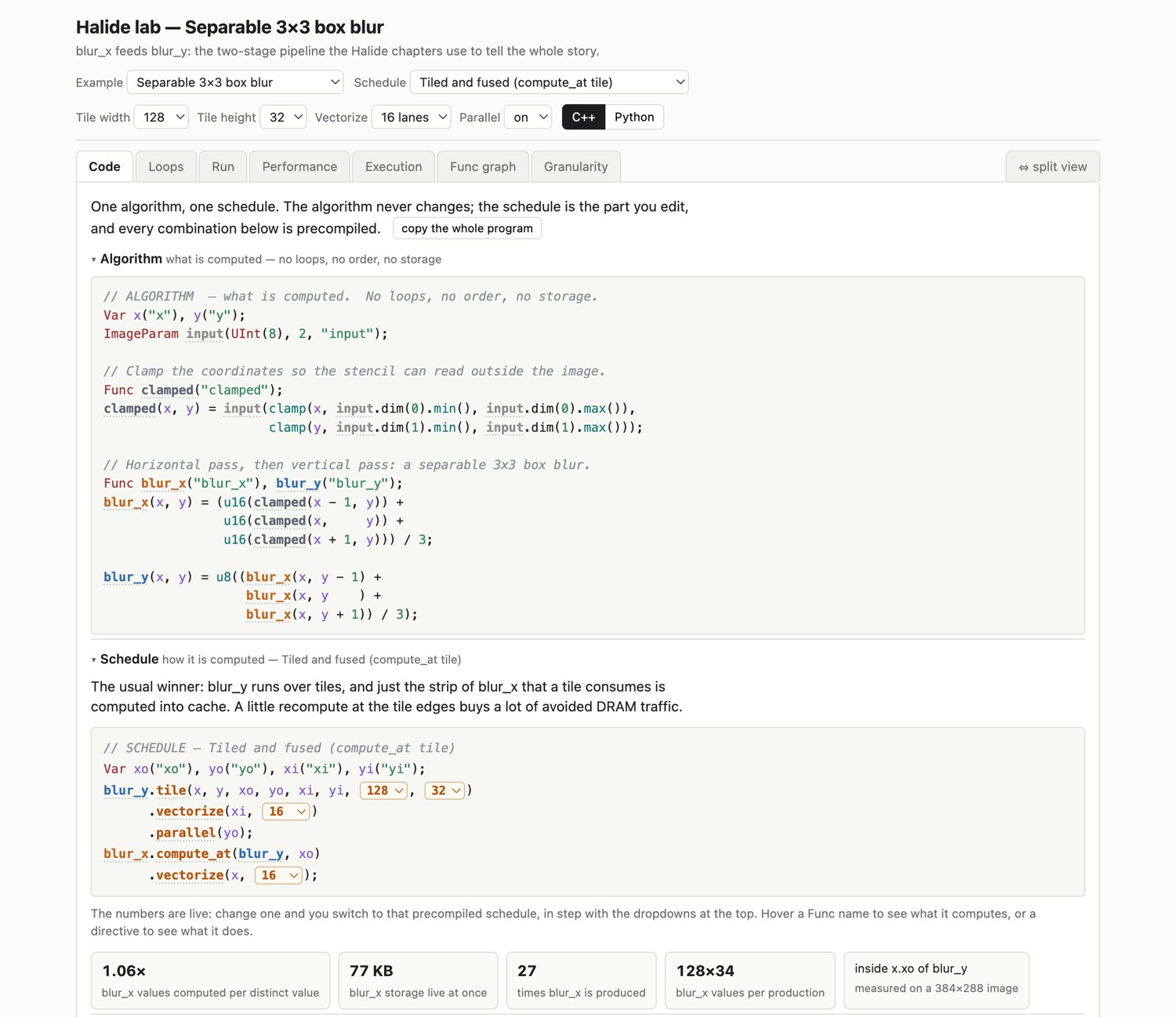
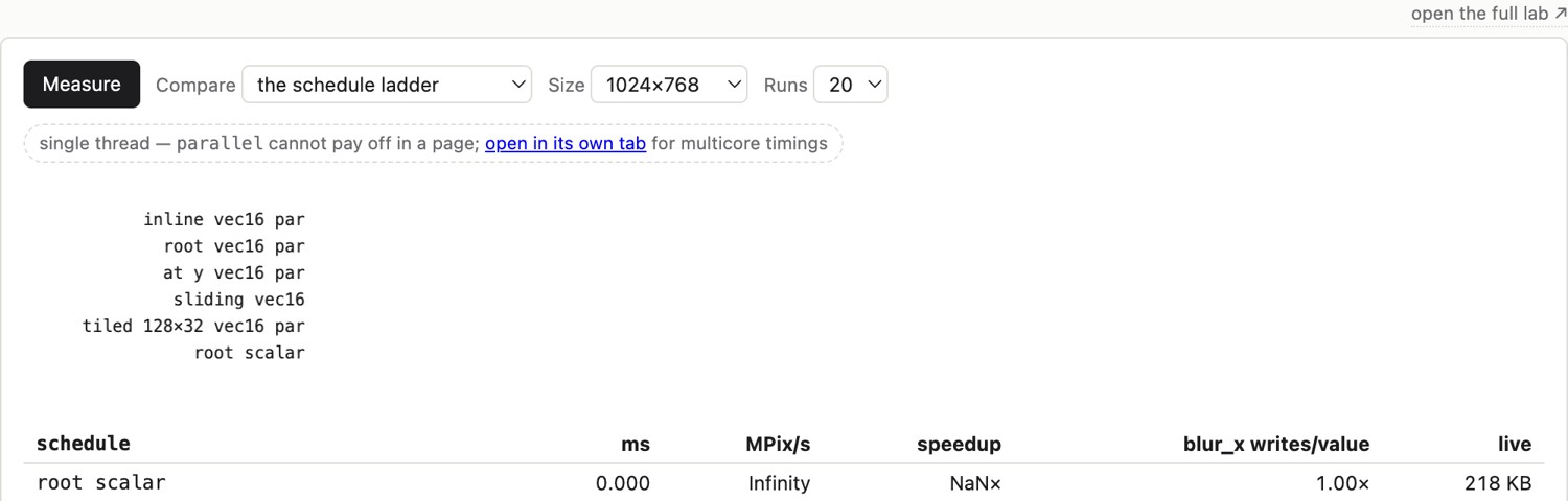
print_loop_nest() prints: the produce/consume structure, which loop runs innermost, and where each stage is computed and stored. This is one extracted view of the lab in Figure 29.4.3, kept in step with it, so changing the schedule or tile size in either updates both.The inline default has a useful consequence for readability: naming a pure intermediate does not automatically allocate an image for it. Split a long expression into stages such as luma, residual, and weight so the algorithm is understandable. Materialize a stage when its reuse justifies storage. The algorithm’s vocabulary can therefore follow the mathematics while the schedule decides which named values need buffers.
Reason about placement from the consumer backward. The output region determines what its stencil asks of the producer. After choosing the consumer’s tile loops, place the producer inside the appropriate loop and let bounds inference propagate the required region upstream. Data values flow forward through the graph, but the demand for them is determined from downstream uses.
29.4.6 Scheduling the loops within a stage: reorder, split, tile, vectorize, unroll, parallel, fuse⧉
For f(x,y), Halide's default pure-stage loop order has x innermost. reorder lists dimensions from inner to outer:
blur_y.reorder(y, x); // y becomes inner, x outerbefore: after reorder(y,x): for y: for x: for x: for y: compute output compute output
Which is faster depends on actual strides and reuse. For conventional row-major storage, adjacent x values are the useful inner traversal.
split introduces outer and inner coordinates. With a split factor of 16, $x=16x_o+x_i$. For arbitrary widths the last group may be partial. This example chooses guarded tails explicitly:
Var xo("xo"), xi("xi");
blur_y.split(x, xo, xi, 16, TailStrategy::GuardWithIf);
for xo in [0,ceil(W/16)):
    for xi in [0,16):
        x = 16*xo + xi
        if x < W: compute output(x,y)
vectorize maps a suitable loop to vector lanes. unroll duplicates a fixed loop body. parallel distributes independent iterations among workers. fuse combines two loop indices into one, often to expose more tasks; this index operation is different from interleaving producer and consumer stages.
A tiled schedule combines two splits and a reorder. Insert this as one alternative in the complete blur program:
Var xo("xo"), yo("yo"), xi("xi"), yi("yi");
blur_y.tile(x, y, xo, yo, xi, yi, 256, 32, TailStrategy::GuardWithIf)
      .vectorize(xi, 8, TailStrategy::GuardWithIf)
      .parallel(yo);
It distributes rows of tiles among workers and uses eight-lane groups along each tile row. Eight is an example, not a universal native width. This schedules only blur_y; it does not automatically vectorize a materialized producer.
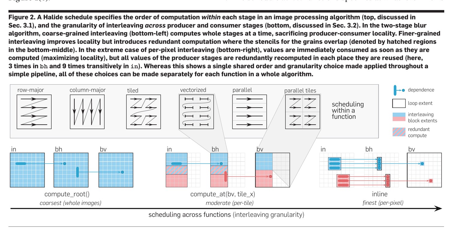
reorder/tile/vectorize/parallel operators of this section). Bottom, scheduling across functions: the producer/consumer granularity for blur_x (bh) feeding blur_y (bv): compute_root (compute whole stages, maximal reuse, full memory traffic), compute_at(bv, tile_x) (per-tile, the balanced middle), and inline (recompute each value where it is used, no storage). Hatched cells are redundantly recomputed; shaded blocks are what is materialized. Reproduced from Ragan-Kelley et al. (Halide, CACM 2018, Fig. 2); Durand is an author, self-granted.For example, vectorization and unrolling can be tried independently before combining them with tiling. Each fragment below is a separate schedule for a freshly constructed blur pipeline:
// Eight adjacent output values in a vector group.
blur_y.vectorize(x, 8, TailStrategy::GuardWithIf);
// Four copies of the inner body, with a guard for the final partial group.
Var xo("xo"), xi("xi");
blur_y.split(x, xo, xi, 4, TailStrategy::GuardWithIf).unroll(xi);
// Independent output rows distributed among workers.
blur_y.parallel(y);
Unrolling duplicates scalar expressions and may expose instruction-level parallelism. Vectorization requests a vector loop, whose lowering depends on the target and operations. Parallelization assigns larger independent chunks to workers. They address different resources, so combining them can help, but each also has costs: larger generated code, tail handling, or task overhead.
For a tiled output, the conceptual loop structure is:
parallel for yo in rows_of_tiles:
    for xo in columns_of_tiles:
        for yi in rows_within_tile:
            for xi_group in groups_of_eight_columns:
                compute eight valid output values
The tile-row loop may expose too few tasks for a short, wide image. Fusing the two outer tile coordinates creates one task index spanning both directions:
Var xo("xo"), yo("yo"), xi("xi"), yi("yi"), tile("tile");
blur_y.tile(x, y, xo, yo, xi, yi, 256, 32, TailStrategy::GuardWithIf)
      .fuse(xo, yo, tile)
      .parallel(tile)
      .vectorize(xi, 8, TailStrategy::GuardWithIf);
This is another alternative schedule, not an additional fragment to append after parallelizing yo. Compare its extra task count and overhead on the dimensions your application processes.
29.4.7 The heart of it: producer-consumer granularity (compute_at, store_at)⧉
For the tiled consumer above, place its horizontal producer inside the xo loop:
blur_x.compute_at(blur_y, xo)
      .vectorize(x, 8, TailStrategy::GuardWithIf);
For a full 256×32 output tile, bounds inference derives a 256×34 horizontal region. The extra rows supply the vertical stencil. For one float channel, the intermediate alone is $256\cdot34\cdot4=34{,}816$ bytes, or 34 KiB. This is not automatically an L1-sized working set once other data and workers are included.
for yo:
    for xo:
        produce the horizontal region needed by this output tile
        for yi:
            for xi:
                compute valid output pixels using that region
Adjacent tile rows overlap in their producer halos, so some work repeats. A taller tile reduces the halo fraction but uses more storage and may leave fewer independent tasks. A very small tile increases scheduling overhead and boundary recomputation.
store_at moves the allocation's lifetime outward relative to computation. Under a suitable access pattern, retaining storage across consumer rows permits sliding-window reuse and folding into a small circular buffer. It does not by itself guarantee a particular buffer size or remove every repeated computation. Chapter 29.5, Scaling up Halide develops the row-buffer case.
compute_at and producer-consumer scheduling in Frédo Durand's performance-engineering lecture; see Video Resources.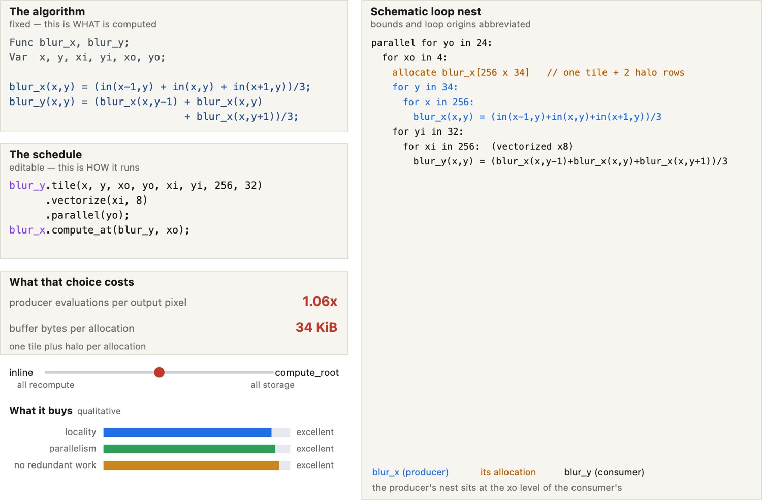
blur_x feeding blur_y. Everything you can change is schedule, and the loop nest on the right is what Halide generates from it, which is the whole point of the language: the two halves are edited independently. Set the consumer's own loops (a plain row-major pass, or tiled, vectorized, parallel), then make the decision that defines Halide: where the producer is computed. inline folds blur_x into blur_y and recomputes every value three times for no memory at all; compute_root() computes the whole image once into DRAM; compute_at puts it in between, materializing only the piece each chunk of the consumer needs. Watch the producer's loop nest move up and down inside the consumer's as you change that choice, and its allocation shrink from the whole image to one tile plus its halo. The halo is the tell that Halide is doing the bounds analysis for you: a vertical 3-tap stencil needs two extra rows, so a $256\times32$ tile of the consumer asks for a $256\times34$ tile of the producer, and the redundancy and live-storage readouts follow from that geometry.Count producer evaluations, distinct needed values, and peak live storage separately. A full interior tile has a geometric halo factor of $34/32=1.0625$; a whole-image ratio also includes image edges and partial tiles. An inline stage may leave no stores to trace, so its arithmetic cannot be counted solely from trace_stores().
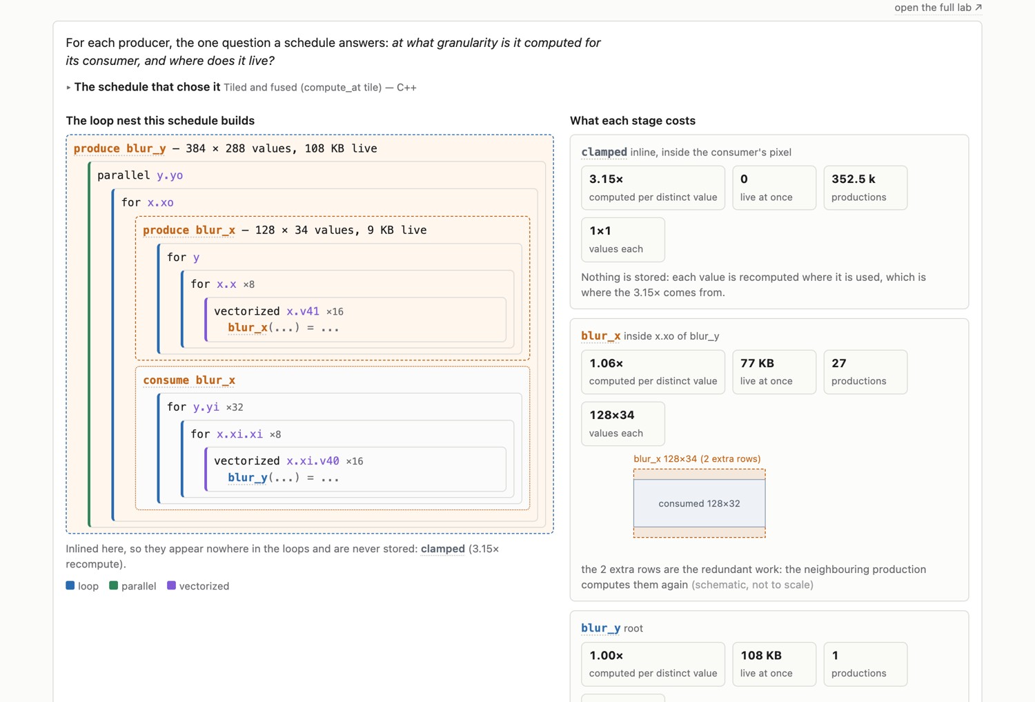
produce sitting at the level compute_at chose, and every stage gets a card: values computed per distinct value, bytes per allocation (with a parallel loop, several allocations can be live at once), number of productions, and the size of one production, with the halo drawn thick enough to see. All four numbers are measured from a trace of that schedule rather than derived from the code, so an inlined stage correctly reports zero storage and its full recompute factor.29.4.8 Comparing schedules with measurements⧉
The lecture records the following historical measurements for a 5×5 separable blur on a 35-megapixel image using a 12-core CPU. They illustrate that scheduling matters; they are not timings of the chapter's 3×3 program.
| Lecture schedule | Time | Speedup over inline |
|---|---|---|
| Inline | 5.81 s | 1.0× |
| Materialize the first stage | 2.00 s | 2.9× |
| Tile and interleave | 1.76 s | 3.3× |
| Tile, parallelize, vectorize; no interleaving | 1.11 s | 5.2× |
| Tile, parallelize, vectorize, interleave | 0.55 s | 10.6× |
Read the table by following one intermediate value through the computation. Under the default inline schedule, its expression is substituted wherever the vertical blur uses it. In the five-tap example, neighboring output rows repeatedly request the same horizontal sums. No horizontal image is stored, but much of its arithmetic is repeated:
for each output pixel:
    compute five horizontal sums from the input
    average those five sums into the output
Materializing the first stage replaces that repetition with reuse. Compute the required horizontal image once, then let every output row read the horizontal values it needs:
// One alternative for a fresh copy of the chapter's blur pipeline.
blur_x.compute_root();
for each required horizontal pixel: compute and store its horizontal sum for each output pixel: average the required stored horizontal sums
The measured drop from 5.81 to 2.00 seconds says that storing this intermediate was cheaper than repeatedly computing it in that experiment. It does not make full-image storage universally desirable. The next schedule keeps reuse while shortening the lifetime of the intermediate: tile the output and produce only the horizontal region that each tile needs.
// Another independent alternative, using this chapter's illustrative tile size.
Var xo("xo"), yo("yo"), xi("xi"), yi("yi");
blur_y.tile(x, y, xo, yo, xi, yi, 256, 32, TailStrategy::GuardWithIf);
blur_x.compute_at(blur_y, xo);
for each output tile:
    compute the tile's horizontal intermediate, including the needed halo
    compute this output tile from that intermediate
    reuse the intermediate storage for the next tile
Now neighboring tiles may repeat some halo work, but a consumer uses its producer soon after the values are made. If the working set fits, the intermediate can remain in cache. The historical single-thread tiled measurement, 1.76 seconds, shows a modest gain over full materialization. This change addresses locality and redundant work; it has not yet asked for vector instructions or multiple workers.
The two faster rows add those forms of parallelism. Vectorization groups adjacent output values into lanes; parallel tiles provide independent work for cores. With a root producer, the horizontal and vertical passes remain separate and need a full intermediate. With a tile-local producer, each task produces and consumes its own region. The latter measured 0.55 seconds, compared with 1.11 seconds for the version without interleaving. The code alternatives below expose both organizations. Producer placement, producer vectorization, and task structure must all be specified before attributing that difference to a single cause.
The slide digest identifies 256×256 tiles for these tiled measurements. The 256×32 code above is an illustrative candidate, not the measured configuration. The separate lecture comparison of a 3×3 blur on a quad-core machine is a different experiment and should not be merged into this table.
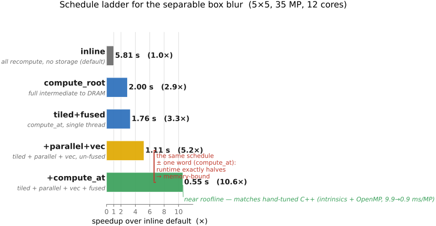
compute_root first stage (2.00 s, ≈2.9×), recompute removed and the full intermediate to DRAM; tiled + fused, single-thread (1.76 s, ≈3.3×), locality only; tiled + parallel + vectorized, un-fused (1.11 s, ≈5.2×), SIMD and cores but memory-bound; tiled + parallel + vectorized + fused (compute_at) (0.55 s, ≈10.6×), the sweet spot, near roofline and matching hand-tuned C++ (the 9.9→0.9 ms/MP, 11× intrinsics version). A bracket highlights the un-fused→fused pair (1.11→0.55 s): the exact doubling that marks the kernel as memory-bound. Timings from the lecture benchmark; the C++ comparison from Ragan-Kelley et al.For a controlled comparison now, fix the algorithm, type, dimensions, boundary rule, target, and thread count. Construct each candidate afresh. To isolate producer placement, hold tile size and vectorization constant and change only the placement. Timing alone suggests a mechanism; traffic measurements or additional experiments are needed to establish it.
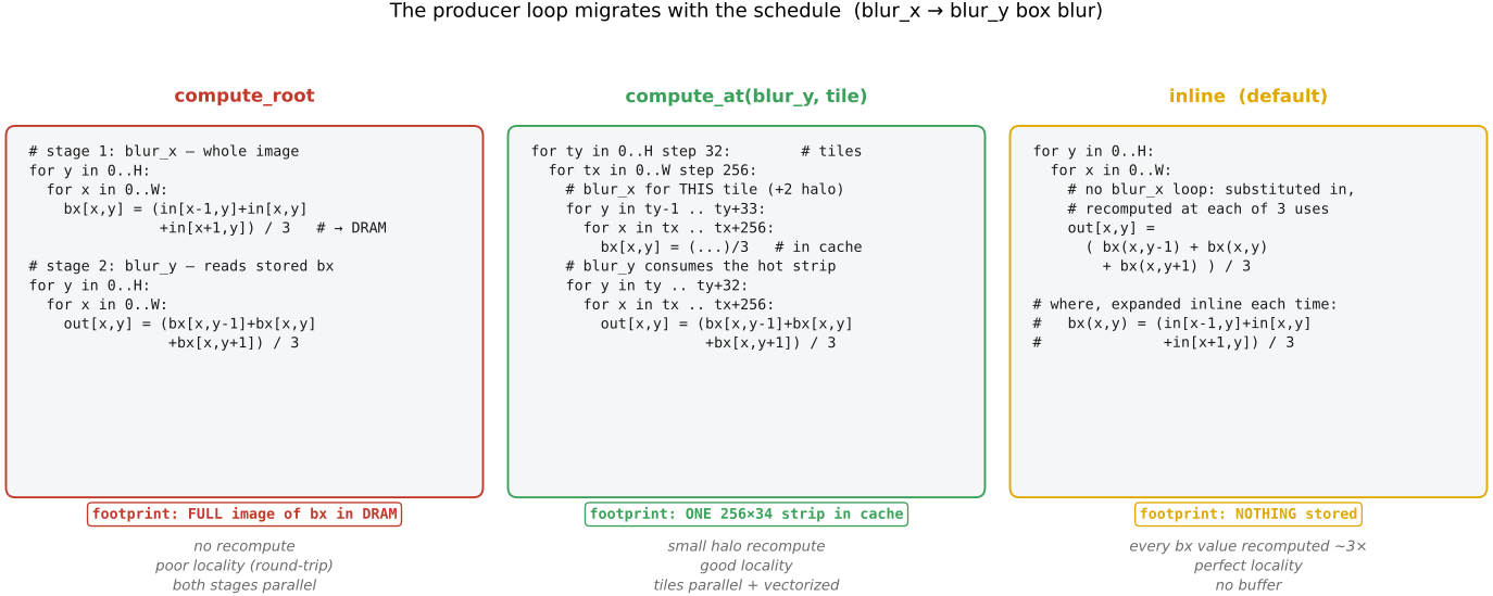
compute_root: two separate loop nests, the whole blur_x computed and stored before any blur_y runs (a full-image buffer between them, $H+2$ rows tall for the halo). Middle, compute_at(blur_y, tile): the blur_x loop nests inside the blur_y tile loop, computing a 256×34 strip (note the +2 halo Halide infers) into a small cache-resident buffer just before the tile of blur_y consumes it. Right, inline: no blur_x loop at all; its expression is substituted directly into blur_y's body, recomputed at every use. The materialized footprint under each (full image, one tile, nothing) is the locality/recompute trade made visual, and lines up rung-for-rung with the speed ladder of Figure 29.4.13. The nests are simplified for reading, not literal compiler output.A different image size or machine can reverse the ordering. Small images may favor inline execution because task and allocation overhead dominate; larger or more expensive producers may favor materialization.
To make the schedule comparison reproducible, here are two alternatives for the chapter's three-tap float blur. Each goes into a fresh copy of the complete program, with the same 256×32 output tiling. They are illustrative experiments, not code attributed to the historical five-tap timing table.
// Full intermediate, with both stages vectorized and parallelized.
Var xo("xo"), yo("yo"), xi("xi"), yi("yi");
blur_y.tile(x, y, xo, yo, xi, yi, 256, 32, TailStrategy::GuardWithIf)
      .vectorize(xi, 8, TailStrategy::GuardWithIf).parallel(yo);
blur_x.compute_root()
      .vectorize(x, 8, TailStrategy::GuardWithIf).parallel(y);
// Per-tile intermediate; output tiles provide parallel work.
Var xo("xo"), yo("yo"), xi("xi"), yi("yi");
blur_y.tile(x, y, xo, yo, xi, yi, 256, 32, TailStrategy::GuardWithIf)
      .vectorize(xi, 8, TailStrategy::GuardWithIf).parallel(yo);
blur_x.compute_at(blur_y, xo)
      .vectorize(x, 8, TailStrategy::GuardWithIf);
In the root case the producer has its own parallel pass. In the tile case producer work runs inside each parallel consumer task. That organizational change affects both storage and task structure, so a runtime difference alone does not isolate a memory-bandwidth mechanism. Inspect allocations and loops, compare numerical outputs, then measure across image sizes. Keeping the two code blocks visible makes their actual differences available for inspection.
29.4.9 Boundaries and bounds⧉
Boundary conditions belong to the algorithm. BoundaryConditions::repeat_edge repeats the nearest valid pixel; constant, mirror, and periodic extensions define different operators. The wrapper in the complete example makes every stencil input access valid for a nonempty image. Real applications should reject unsupported empty inputs before constructing or running the pipeline.
Bounds inference determines which producer coordinates consumers require. It does not invent a boundary policy or automatically clamp every access. Tail handling is another issue: a split whose factor does not divide the extent needs guards, shifted tiles, or another legal tail strategy. The explicit guarded strategy above handles partial groups without changing the boundary extension.
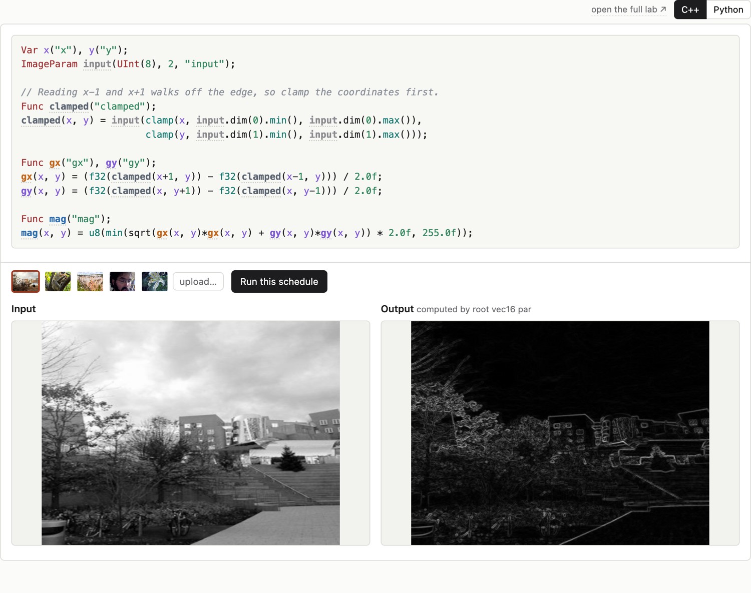
clamped) becomes an ordinary Func like any other, inlined by default. Switch the schedule to see the two gradients materialized instead, and run it on a photograph.Input buffers may have nonzero minima and arbitrary strides. The examples assume zero minima; for general buffers, derive domains from their dimension metadata. Test 1×1, 1×N, non-square, odd-sized, and cropped inputs. Compiler loop partitioning can reduce boundary-check overhead, but it does not guarantee that every check disappears.
29.4.10 Same algorithm, new machine: the GPU⧉
For a GPU target, gpu_tile maps independent output work to block and thread coordinates. A minimal alternative is to keep the pure horizontal producer inline and tile only the output:
Var bx("bx"), by("by"), tx("tx"), ty("ty");
blur_y.gpu_tile(x, y, bx, by, tx, ty, 16, 16,
                TailStrategy::GuardWithIf);
This schedule requires a configured GPU target when compiling or realizing. It is a baseline: repeated producer work may be expensive. A more elaborate schedule can compute the producer per block and explicitly arrange shared-memory storage and cooperative thread work.
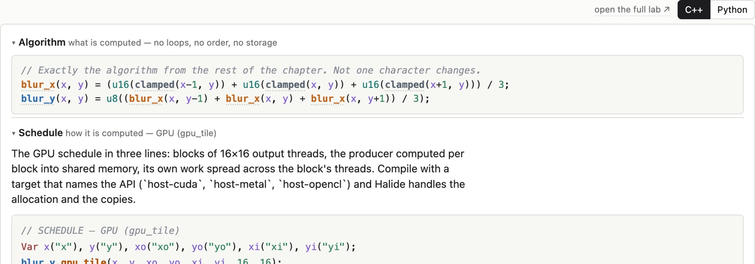
host-cuda, host-metal or host-opencl and Halide handles the allocation and the copies.compute_at specifies loop placement, not a universal request for GPU shared memory. The target, storage choice, synchronization, and producer schedule must agree. Include host-device transfers and synchronization in end-to-end timing; see the GPU tutorial.
29.4.11 Letting the compiler schedule: the auto-scheduler⧉
Autoschedulers generate candidate schedules from the pipeline, target, and estimates of representative input/output sizes. Analytical and learned models are described by Mullapudi and colleagues Mullapudi et al. 2016 and Adams and colleagues Adams et al. 2019. Runtime and quality of the generated schedule depend on the plugin and workload.
Use a fresh unscheduled pipeline for an autoscheduler unless its documentation explicitly supports partial manual schedules. Supply realistic estimates, then benchmark on actual dimensions. Estimates guide optimization; they are not generally runtime bounds or correctness constraints. Compare the result with simple manual baselines before deciding where further tuning is worthwhile.
The search is difficult because choices interact. Inlining a producer can remove its buffer but multiply work at each consumer. Tiling a consumer changes the region the producer needs, and a vector width can constrain useful tile sizes. An autoscheduler estimates these consequences while exploring candidate organizations. An analytical cost model expresses the expected costs directly; a learned model estimates them from examples of measured schedules. Neither model knows the intended workload unless the pipeline, target, and size estimates describe it. Inspecting and benchmarking the selected schedule connects the automated search back to the same locality, parallelism, and recomputation tradeoffs used by a human.
29.4.12 A repeatable scheduling experiment⧉
Keep a small reference implementation and saved baseline timings. For each schedule, check output differences, inspect the loops, then measure with tracing disabled and compilation outside the steady-state interval. Record enough configuration to reproduce the comparison. This becomes more important when Chapter 29.5, Scaling up Halide adds reductions, shared producers, and several resolutions.