29.3 Halide at a high level: decoupling algorithms from schedules⧉
A separable blur is easy to express as two loops: compute horizontal averages, then vertical averages. Optimizing it may require interleaving those loops, retaining a few rows, recomputing tile halos, and distributing work across vector lanes and cores. The formula becomes hard to recognize inside the resulting indexing code.
The difficulty grows with the pipeline. Each stage offers many independent pixels, but a succession of inexpensive stages can spend more time moving intermediate images than evaluating formulas. Writing the whole horizontal image before beginning the vertical pass gives clear code and a large intermediate. Interleaving the passes makes the intermediate smaller, but their loop nests become entangled. Tile boundaries need extra rows, vector instructions need groups of adjacent pixels, and parallel tasks need independent storage.
An optimized implementation now contains two kinds of knowledge in the same code: the filter that defines the answer and the organization that suits the machine. Change the stencil and the halo calculations need revisiting. Change the hardware and the tile sizes, vector width, and task layout may need revisiting. A programmer trying to understand the image operation has to read through all of those choices. The cost is maintenance as well as the time spent finding the fast implementation.
Halide separates these concerns. The algorithm describes stage values; the schedule specifies how to evaluate and retain them. This chapter follows the language and scheduling ideas in Ragan-Kelley and colleagues' papers [@ragan-kelley-etal-2012; @ragan-kelley-etal-2013; @ragan-kelley-etal-2018-cacm]. The practical syntax follows in Chapter 29.4, Halide programming.
Legal schedules preserve the algorithm's semantics, but this is not a blanket promise of bitwise agreement across floating-point transformations, targets, or reduction orders. Input bounds and layouts must also satisfy the compiled pipeline's requirements. A schedule changes executed work as well as data movement when it introduces or removes recomputation.
Write the pixel computation clearly, then vary how its values are produced, stored, and reused. A separate schedule makes optimization easier to inspect and retarget; it does not remove the need to measure or validate the result.
The split makes experiments cheaper. Keep the formulas and try a full intermediate, a tiled intermediate, or a sliding row buffer by changing a compact schedule. Someone who understands the application can work on the formulas while someone who understands the target studies their execution. The separation does not choose a good schedule automatically; it gives both people a representation in which a scheduling change is visible as such, instead of being buried in a rewritten image loop.
This also explains the value of retargeting. A CPU schedule might use vectorized rows and parallel tiles; a GPU schedule maps work to blocks and threads and chooses storage appropriate to that target. Much of the algorithm can remain recognizable across the two implementations. Target support, numerical behavior, and boundary requirements still need checking, but changing the machine need not mean expressing the entire photographic operation again Ragan-Kelley et al. 2018 (CACM).
29.3.1 Images as pure functions⧉
A pure Halide Func maps integer coordinates to values. Its definition does not allocate an image or enumerate pixels. The requested output region and dependencies determine which coordinates must be evaluated. Input buffers remain finite, so the algorithm must define boundary behavior or restrict the output domain.
Here is a floating-point 3×3 box blur, with repeated-edge boundaries on a two-dimensional input:
using namespace Halide;
Var x("x"), y("y");
ImageParam input(Float(32), 2, "input");
Func bounded = BoundaryConditions::repeat_edge(input);
Func horizontal("horizontal"), output("output");
horizontal(x, y) = (bounded(x-1, y) + bounded(x, y)
                    + bounded(x+1, y)) / 3.0f;
output(x, y) = (horizontal(x, y-1) + horizontal(x, y)
               + horizontal(x, y+1)) / 3.0f;
The divisions matter: omitting both gives a nine-sample sum rather than an average. For integer input, widen before adding; casting an already-overflowed sum is too late.
Update definitions extend this model to reductions, histograms, and scans. An update has ordering and dependency constraints; not every update is an associative reduction or freely parallelizable. A histogram increments a data-dependent bin; a cumulative sum depends on the previous bin. Chapter 29.4, Halide programming and Chapter 29.5, Scaling up Halide give concrete examples.
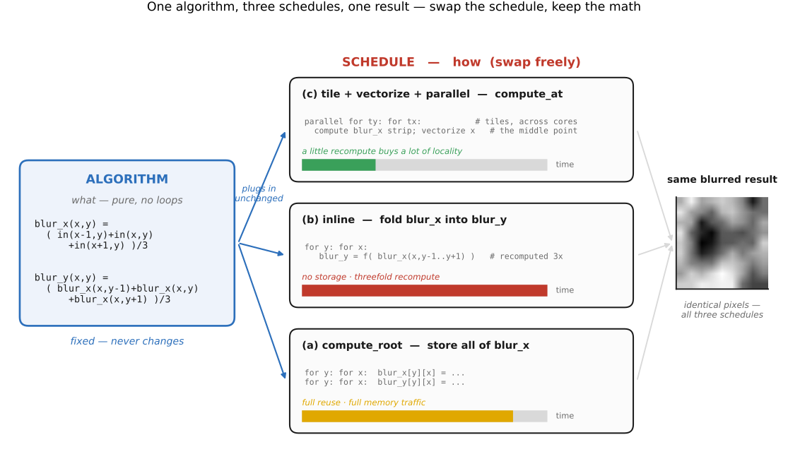
blur_x → blur_y), with no loops, the unchanging definition of what is computed. On the right, three schedule boxes, each a few lines, that the algorithm box plugs into unchanged: (a) store all of blur_x, including the two extra halo rows blur_y needs, then run blur_y (full reuse, full memory traffic); (b) inline blur_x into blur_y (no storage, threefold recompute); (c) compute blur_x per tile, vectorized and parallel (the middle point). Below each, the loop nest it generates and a relative timing bar; above all three, the same blurred output image, identical pixels, very different speed. (Schematic.)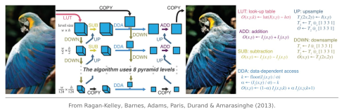
A histogram followed by a cumulative sum shows why update definitions carry different dependencies. This fragment assumes a nonempty, zero-origin two-dimensional unsigned 8-bit input buffer named input8:
using namespace Halide;
Var bin("bin");
Func histogram("histogram"), cumulative("cumulative");
RDom pixels(0, input8.width(), 0, input8.height(), "pixels");
histogram(bin) = cast<int64_t>(0);
histogram(cast<int32_t>(input8(pixels.x, pixels.y))) += cast<int64_t>(1);

cumulative(bin) = cast<int64_t>(0);
cumulative(0) = histogram(0);
RDom bins(1, 255, "bins");  // bins 1 through 255, inclusive
cumulative(bins) = cumulative(bins-1) + histogram(bins);
histogram.compute_root();
cumulative.compute_root();
The histogram update scatters into a bin selected by each sample. The cumulative update visits bins in order and reads the preceding result. Bin zero must be initialized from its histogram count, and the final cumulative value at bin 255 should equal the total number of pixels. Parallelizing either update blindly is incorrect: histogram writes can collide, while the cumulative sum has an explicit dependence. A different parallel formulation is possible, but it must preserve those semantics.
The chain ends with a gather. Each output pixel looks up the cumulative count of its own input value and scales it to the output range, which is histogram equalization:
Var x("x"), y("y");
Func equalized("equalized");
Expr total = cast<double>(input8.width()) * cast<double>(input8.height());
Expr rank  = cast<double>(cumulative(cast<int32_t>(input8(x, y))));
equalized(x, y) = cast<uint8_t>(clamp(255.0 * rank / total + 0.5, 0.0, 255.0));
Scatter, scan, gather: three stages with three different dependence patterns. The scatter needs protection from colliding writes, the scan is ordered, and the gather is fully parallel across pixels, reading a 256-entry table that fits in any cache. A schedule that treats them alike, all inlined or all parallelized, is either wrong or slow, which is why each stage gets its own schedule. This simple mapping sends the darkest occupied value above zero; subtracting the first nonzero cumulative count before normalizing stretches the output to the full range.
The coordinates need not describe a two-dimensional photograph. A Func can describe a one-dimensional curve, a three-dimensional bilateral grid, or a tuple of values at each position. This is why the language’s useful restriction is to regular multidimensional computations rather than to photography as an application. Expressing stages as values and dependencies gives the compiler a structure on which loop and storage transformations can operate.
29.3.2 The schedule: four questions for every stage⧉
A schedule answers four questions: in what order are values computed, how are they laid out, where is a producer computed relative to its consumers, and how long is its storage retained?
Within a stage, loops can be split, reordered, tiled, vectorized, unrolled, and parallelized where dependencies permit. Storage layout is a separate choice. A good loop order follows useful memory strides; a reduction may constrain which axes can run independently.
Across stages, consider the horizontal producer above. Inlining substitutes its expression at each use. There is no producer buffer, but neighboring vertical outputs ask for overlapping producer rows, so work may repeat. Input loads still occur and their cache behavior still matters.
With horizontal.compute_root(), the required horizontal region is computed before the output. Each stored producer value can serve several output rows. This avoids that recomputation at the cost of an intermediate whose size grows with the requested image.
For a tiled consumer, compute_at places production inside a chosen tile loop. A 256×32 output tile needs a 256×34 horizontal region for the centered vertical three-tap stencil. That is 34 KiB for one float channel, before other live data. Neighboring tile rows overlap in two producer rows. For full interior tiles the producer-work ratio relative to tile area is $34/32=1.0625$, ignoring outer-image and tail effects.
for each output tile:
    produce horizontal values for the tile plus its vertical halo
    compute this output tile from those values
    release the tile's intermediate storage
store_at can retain a producer's allocation outside the loop where compute_at computes it. If the access pattern permits sliding-window reuse and storage folding, a few rows can be retained while successive output rows advance. Storage lifetime, computation frequency, and buffer size are related but distinct choices. The multistage scheduling tutorial shows their effects on generated loops.
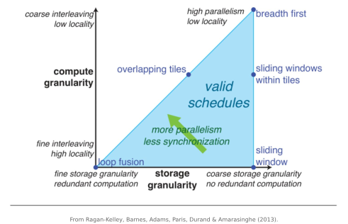
compute_root) at the coarse/coarse corner (high parallelism, no recompute, low locality), with overlapping tiles and sliding windows in between. Moving toward more parallelism and locality costs redundant computation: you cannot reach every corner at once, and a schedule is the choice of where to stand. Reproduced from Ragan-Kelley et al. (Halide, PLDI 2013 / CACM 2018); Durand is an author, self-granted.Writing the two extreme loop nests makes the difference visible. In these pseudocode listings, bounded implements the same boundary rule as the algorithm, and intervals are half-open.
# Inline: substitute the horizontal formula at each use.
for y in [0,H):
    for x in [0,W):
        output(x,y) = 0
        for dy in [-1,2):
            output(x,y) += (bounded(x-1,y+dy) + bounded(x,y+dy)
                            + bounded(x+1,y+dy)) / 9
# Root: retain the entire required horizontal region.
allocate horizontal for [0,W) × [-1,H+1)
for y in [-1,H+1):
    for x in [0,W):
        horizontal(x,y) = (bounded(x-1,y) + bounded(x,y)
                            + bounded(x+1,y)) / 3
for y in [0,H):
    for x in [0,W):
        output(x,y) = (horizontal(x,y-1) + horizontal(x,y)
                        + horizontal(x,y+1)) / 3
Consider one horizontal value away from the boundary. Three neighboring output rows request it. Root computes and stores it once, then reads it three times; the direct inline expansion recomputes it at each request. Tiled production limits the stored region while reusing values inside the tile. At tile boundaries some producer rows are computed again. The compiler can simplify the expanded arithmetic further, but these loop nests explain the scheduling decision before such optimizations.
The extremes make the tradeoff look harsher than it often is. Full inlining can repeat too much work; full materialization can retain too much data. An intermediate tile or sliding window may recover much of the reuse while keeping enough independent work for the machine. The purpose of the schedule is to explore those intermediate choices cheaply, including different choices at different producer-consumer boundaries.
Computation order and storage order are independent choices. A loop can visit pixels along x even if the buffer has a different contiguous dimension, though the resulting strides may waste bandwidth. Splitting a loop introduces a coarse and a fine coordinate; reordering those loops makes a tiled traversal; mapping a fine coordinate to vector lanes exposes data parallelism. These operations reorganize one stage. Moving its production inside a consumer loop changes the relationship between stages.
The same distinction applies to a longer graph. A producer used twice inside a tile may be worth materializing there, while an inexpensive producer used only once may be cheaper inline. A coarse pyramid level may fit comfortably as a complete image while the finest level needs tiling. There is an execution choice at every stage and a reuse question at every producer-consumer connection. Applying one schedule pattern uniformly can miss the different costs at those connections.
29.3.3 What the compiler derives⧉
Halide lowers the algorithm and schedule into loops, allocations, and target code. Bounds inference propagates required output regions backward through producer accesses, deriving intermediate regions and halos. A programmer no longer has to maintain that indexing arithmetic by hand for each tile size.
The compiler still makes consequential decisions: simplification, common-expression elimination, loop partitioning, storage folding where legal, and target instruction selection. LLVM and target backends add further optimization. A manual schedule controls major organization choices; it does not specify every generated instruction Ragan-Kelley et al. 2013.
29.3.4 What the split buys, measured⧉
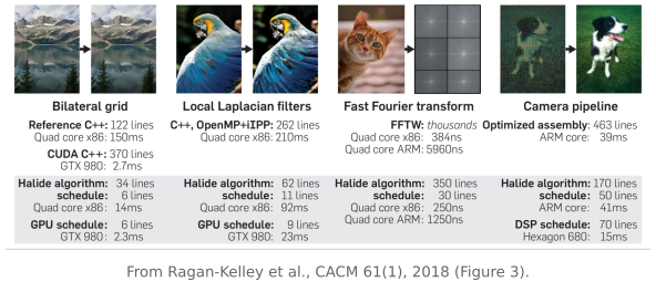
The 2018 CACM account compares four pipelines with expert implementations on the hardware used in that study (Figure 29.3.2) Ragan-Kelley et al. 2018 (CACM). The table separates algorithm code from scheduling code. The CPU, GPU, and DSP rows are different targets, not a controlled comparison on one processor.
| Pipeline | Reference | Halide | Result |
|---|---|---|---|
| Bilateral grid Chen et al. 2007 | 122 lines C++, 150 ms | 34 lines + 6 of schedule, 14 ms | 11× |
| same, GPU | 370 lines CUDA, 2.7 ms | + 6 lines of GPU schedule, 2.3 ms | 17% faster, a tenth of the code |
| Local Laplacian filters Paris et al. 2011 | 262 lines C++ with OpenMP and Intel IPP, 210 ms | 62 lines + 11 of schedule, 92 ms | 2.3× |
| same, GPU | + 9 lines of GPU schedule, 23 ms | 9.1× the tuned CPU reference | |
| Fast Fourier transform | FFTW, thousands of lines, 384 ns per 16×16 tile | 350 lines + 30 of schedule, 250 ns | 1.5× on x86, up to 4.6× on ARM |
| Camera pipeline Adams et al. 2010 (Frankencamera) | 463 lines of ARM assembly and intrinsics, 39 ms | 170 lines + 50 of schedule, 41 ms | parity on one core, 2.7× on four |
| same, DSP | 70 lines of schedule, 15 ms | four-core speed at up to ten times less power |
The implementation details explain why the schedules differ.
The bilateral grid reference is a clean, tuned implementation by the algorithm's own authors. GCC autovectorizes part of it, but it is hard to thread: a naive OpenMP parallelization of the major stages made it slower, so the reference runs on one core. The Halide version gets its 11× from parallelism, tile-level fusion of some stages, and reordering dimensions to control the parallel grain size in the grid. Against 370 lines of hand-written CUDA from the same authors, a different six-line schedule was 17% faster, and it won by doing something its authors had not thought to try: giving up some parallelism in the grid-construction step to cut synchronization overhead, and passing intermediate results through scratchpad memory with a tiled fusion strategy. The example shows why maximizing parallelism at every stage need not minimize the time of the whole pipeline.
The local Laplacian filter is 99 stages operating at many scales, with data-dependent resampling from processed pyramids. The reference is Adobe's: 262 lines, carefully parallelized with OpenMP, with the hot kernels offloaded to Intel's IPP primitives, and it took months to develop, two to three weeks of that on optimization alone. It is already 10× faster than the same algorithm in clean C++ without IPP and OpenMP. The Halide version was written in a day, and its 11 lines of schedule mix different fusion, tiling, vectorization and threading strategies across the 99 stages; in C those 11 lines would be hundreds of loops over thousands of lines. Recompiled with a different schedule it becomes a hybrid CPU/GPU program with 23 distinct GPU kernels, 9.1× the Adobe implementation and 4× the best CPU version.
The FFT is the case where Halide competes with a library rather than with application code. It computes small tiled 2D transforms by running Cooley-Tukey on columns, transposing repeatedly so every transform is over columns, and doing real transforms as pairs of columns. Against FFTW it is about 1.3× on small complex transforms, 1.5× to 2.1× on real ones on x86, and up to 4.6× on ARM, then falls back to parity around 64×64 because no one wrote a vectorization strategy for the larger sizes. A call to a separately compiled FFT library generally creates a fusion boundary: because the transform is ordinary Halide code, whatever you do in the Fourier domain can be fused into the transform itself, and changing it to fixed point or zero-padded is an edit rather than a new library.
The camera pipeline does hot-pixel suppression, demosaicking, color correction and global tone mapping; the demosaicking alone is 21 interdependent stencils. The reference is the Frankencamera's: one carefully tiled and fused loop nest, 463 lines of C++ with ARM NEON intrinsics and inline assembly, every producer-consumer communication staged through scratch buffers by hand. The Halide version is 170 lines describing 32 functions and 22 stencils, translated literally from the pseudocode in the reference's own comments. With 70 more lines of schedule it targets 32- and 64-bit x86, ARM, and Qualcomm's Hexagon DSP. On a Pixel phone, Halide on one ARM core matches the hand-written reference, four cores give 2.7× (against a theoretical 3.5× on those asymmetric cores), and the Hexagon 680 matches the four-core CPU while drawing up to ten times less power in the reported comparison. Porting to the DSP meant replacing tiling with a sliding window over rows, because Hexagon's vectors are very wide and it leans on loop pipelining, so efficient 2D tiles no longer fit in cache. In Halide that is a schedule edit. In the hand-written ARM version it would be a rewrite: the tiling logic reaches all the way into the indexing arithmetic of the assembly inner loops.
29.3.5 How long does a schedule take to write?⧉
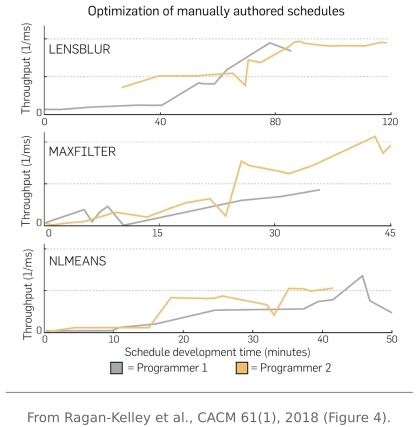
The CACM article describes two experienced developers scheduling three unfamiliar pipelines while recording performance over development time Ragan-Kelley et al. 2018 (CACM). It is evidence about those sessions, not an estimate of how long a new user will need.
The practical method is repeatable: start from a baseline, inspect the loops, change a scheduling choice, and measure. Keep the best known version. An attractive tile geometry can lose to a simpler row schedule because of vector width, task overhead, or the producer's cost.
29.3.6 Where it ended up⧉
MIT released Halide as open source in 2012, and Google became its largest user and contributor. As reported in 2018 Ragan-Kelley et al. 2018 (CACM), Google's HDR+ burst pipeline Hasinoff et al. 2016 was the largest Halide program known, producing the photographs on Pixel phones, and Halide also ran at scale in Google Photos and YouTube. Instagram, Facebook and Adobe shipped it in products; the local Laplacian filter used as a benchmark earlier in this part became part of the clarity and tone controls in Photoshop and Lightroom. The Hexagon DSP backend was built with Qualcomm. These are dated examples, and current products and deployment counts change, but they show a language written to make image kernels easier to optimize running on servers and phones at very large scale.
The separation between an algorithm and its execution schedule traveled further than the language. Machine-learning compilers adopted it: TVM's tensor expression language started from Halide's intermediate representation and its compute/schedule split, then added scheduling primitives for nested parallelism and tensorization that Halide's model did not have. Its value is broader than photography: regular array computations expose reusable structure that a compiler can map to different machines.
29.3.7 Letting the compiler find the schedule⧉
An explicit scheduling space can be searched automatically. Mullapudi and colleagues use an analytical cost model Mullapudi et al. 2016; Adams and colleagues combine a learned cost model with tree search Adams et al. 2019. The search estimates which organizations will run well without exhaustively compiling and timing every possibility.
Treat an autoschedule as a candidate. Provide representative size estimates, check support for the target and pipeline constructs, and measure the result on the intended workload. A good manual schedule and an autoschedule are useful baselines for each other.
Making the schedule explicit gives a search algorithm a vocabulary of choices and a way to generate candidates. The cost model judges locality, parallel work, and recomputation within that representation. This is broader than automating a few tuning constants: the compiler can compare different organizations of the same algorithm. The quality of the search still depends on what its representation permits and what its cost model predicts.
29.3.8 The split was always there, done by hand⧉
Chapter 45.33, Photoshop 1.0, running shows an earlier division of labor between application code and specialized assembly kernels. Such implementations separate concerns socially and by language, but a human must keep optimized code consistent with the intended operation. Halide represents that relationship inside the compiler: the schedule generates an implementation of the algorithm.
29.3.9 Gradient Halide: differentiating the pipeline⧉
Differentiable Halide generates derivative computations for supported pipelines and schedules those computations too Li et al. 2018. This permits fitting filter coefficients or other continuous parameters by gradient descent, and combining engineered image operators with learned components.
Differentiation has its own limits. Quantization, discrete choices, and data-dependent indexing are not automatically smooth trainable operations; boundary and derivative conventions matter. A generated gradient needs validation, just as a generated forward pipeline does.
The generated derivative is another pipeline, with its own intermediates and reuse opportunities. Scheduling the forward computation well does not automatically schedule that derivative well. Conversely, having both in the same representation permits an engineered image operator to participate in a learned system without treating its backward computation as an unrelated implementation. Continuous parameters in a classical filter or tone mapping stage can then be fitted against an image loss.
29.3.10 When to use the split⧉
The split is most useful when you need to explore several execution strategies or maintain one algorithm across targets. Use Chapter 29.4, Halide programming to build and inspect those strategies. Keep host-side I/O and application control around the kernels, and preserve a reference result while tuning.
Recap: big lessons of this chapter
Write the pixel computation clearly, then vary how its values are produced, stored, and reused. A separate schedule makes optimization easier to inspect and retarget; it does not remove the need to measure or validate the result.